Efficient Feature Selection and Classification Technique For Large Data

(1)

CSEIT1722314 | Received : 16 April 2017 | Accepted : 26 April 2017 | March-April-2017 [(2)2: 1041-1047]

1041

Efficient Feature Selection and Classification Technique For

Large Data

1P. Arumugam

,

_{P. Jose}2

1

Department of Statistics, Manonmaniam Sundaranar University, Tirunelveli, Tamilnadu, India 2

Research scholar, Department of Statistics, Manonmaniam Sundaranar University, Tirunelveli, Tamilnadu, India

ABSTRACT

Grey wolf optimizer (GWO) is a Heuristic evolutionary algorithm recently proposed, it is inspired by the leadership hierarchy and hunting mechanism of grey wolves in nature. In order to reduce the data set without affecting the classifier accuracy. The feature selection plays a vital role in large datasets and which increases the efficiency of classification to choose the important features for high dimensional classification, when those features are irrelevant or correlated. Therefore, feature selection is considered to use in pre-processing before applying classifier to a data set. Thus, this good choice of feature selection leads to the high classification accuracy and minimize computational cost. Though different kinds of feature selection methods are investigate for selecting and fitting features, the best algorithm should be preferred to maximize the accuracy of the classification. This paper proposes intelligent optimization methods, which simultaneously determines the parameter values while discovering a subset of features to increase SVM classification accuracy. In this paper, initial subset selection is based on the latest bio inspired Grey wolf optimization technique proposed. Which take off the hunting process of gray wolve. This optimizer search the feature space for optimal feature solution in diverse directions in order to minimize the option of trapped in local minimum and enhance the convergence speed. The Novel approach aimed to speed up the training time and optimize the SVM classifier accuracy automatically. The proposed model used to select minimum number of features and providing high classification accuracy of large datasets.

Keywords: Feature Selection, Classification, PSO, GWO , SVM

I.

INTRODUCTION

Building accurate and efficient classifiers for large databases is one of the essential tasks of data mining and machine learning research. Usually, classification is a preliminary data analysis step for examining a set of cases to see if they can be grouped based on similarity to each other. The ultimate reason for doing classification is to increase understanding of the domain or to improve predictions compared to unclassified data. Many types of classification techniques have been proposed in literature that includes DT-SVM, SMO, etc. SVM is a learning machine used as a tool for data classification, Function approximation, etc., due to its generalization ability and has found success in many applications [7-11]. Feature of SVM is that it minimizes and upper bound of

(2)

whatever processes distinguish the classes. In this paper, we concentrate on GWO, developed by Mirjalili et al. [7] in 2014 based on simulating hunting behavior and social leadership of grey wolves in nature. Numerical comparisons showed that the superior performance of GWO is competitive to that of other population-based algorithms. Because it is simple and easy to implement and has fewer control parameters, GWO has caused much attention and has been used to solve a number of practical optimization problems [16– 18]. However, like other stochastic optimization algorithms, such as PSO and GA, as the growth of the search space dimension, GWO algorithm provides a poor convergence behavior at exploitation [19, 20].Therefore, it is necessary to emphasize that our work falls in increasing the local search ability of GWO algorithm According to [21].

1. Support Vector Machine

SVM structured as a two-class problem, where the classes are separable linearly. The input dataset D be represent in 2D as (x1, y1), (x2, y2)…. (x|D|, y|D|), where xi is the set of training tuples and yi is the class label associated with training sample. In a training sample, SVM constructs a line of separation for two attributes (x, y) and a plane of separation for three attributes and a hyper plane of separation for n dimensions. To make the SVM optimization problem accurately obedient by writing Minimize in Equation (1), where 𝜀

∑ (𝜀) (1)

2. Grey Wolf Optimization

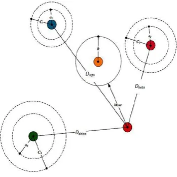
GWO algorithm consider alpha (α) wolves are the fittest solution inside the pack, while the second and third best solutions are named Beta (β) and delta (δ) respectively. The result of solutions inside the pack (population) are considered omega (ω). The process of hunting a prey is guided by α, β and ω.

The first step of hunting a prey is circling it by α, β and

ω. The mathematical model of circling process as shown in equations 2.

X( t+1) = Xp (t) + A⋅D (2)

Where X is the grey wolf position. t is the number of iteration. p X is prey position and D is evaluated from Equation (3).

D=|C.Xp(t+1)-x(t)| (3)

The A and C are coefficient vectors are evaluated based on Equations (4) and (5) respectively.

A = 2a ⋅r1 − a (4)

C = 2r2 (5)

Where a is a linearly decreased from 2 to 0 through the number of iterations, which is used to control the tradeoff between exploration and exploitation. Equation (6) used to update the value of variable a, where NumIter is the total number of iterations. Two random vectors between [0,1] namely 1 r and 2 r to simulate hunting a prey (find the optimal solution). The solutions alpha, beta and delta are considered to have a good knowledge about the potential location of prey. These three solutions helps others wolves (omega) to update their positions according to the position of alpha, beta and delta. Equation 6 presents the formula of updating wolves’ positions.

a = 2 − t (2 NumIter ) (6) X t +1 = X 1+ X 2+ X 3 (7)

The values of X1, X2 and X3 is evaluated as in Equations (8) (9) and (10) respectively.

X1 = |Xα– A1 Dα | (8) X2 = |Xβ– A2⋅Dβ | (9) X3 = |Xδ– A3⋅D δ | (10)

The X1, X2 and X3 are the best 3 solutions in the population at iteration t. The values of A1, A2 and A3 are evaluated in Equation (3). The values of D α, D β

and D δ are evaluated as shown in Equations (11) (12) and (13) respectively.

D α= |C1⋅X α– X| (11)

Dβ= |C2⋅Xβ– X| (12)

Dδ= |C2⋅Xδ– X| (13)

(3)

wolves is divided into four groups: alpha (a), beta (b), delta (d), and omega (w). In every iteration, the first three best candidate solutions are named a, b, and d. The rest of the grey wolves are considered as w, and are guided by a, b, and d to find the better solutions. The mathematical model of the w wolves’ encircling

process is as follows

1) Social hierarchy

In the mathematical model of the social hierarchy of the grey wolves, alpha (α) is considered as the fittest solution. Accordingly, the second best solution is named beta (β) and third best solution is named delta (δ) respectively. The candidate solutions that are left over are taken as omega (ω). In the GWO, the optimization (hunting) is guided by alpha, beta, and delta. The omega wolves have to follow these wolves.

2) Encircling Prey

The grey wolves encircle prey during the hunt. The encircling behavior can be mathematically modeled as follows [18]

Where A and C are coefficient vectors, X p is the preys position vector, X denotes the grey wolf’s position vector and „t‟ is the current iteration. The calculation of vectors A and C is done as follows in Equation (14),(15)

A = 2. a . r 1. a (14) C = 2. r 2 (15) Where values of „a ‟are linearly reduced from 2 to 0 during the course of iterations and r1, r2 are arbitrary vectors in gap [0, 1].

3) Hunting

The hunt is usually guided by the alpha, beta and delta, which have better knowledge about the potential location of prey. The other search agents must update their positions according to best search agents position. The update of their agent position can be formulated as follows [18]:

4) Search for prey and attacking prey

The A is an arbitrary value in the gap [-2a, 2a].

 When |A| < 1, the wolves are forced to attack the prey. Attacking the prey is the exploitation ability and searching for prey is the exploration ability. The random values of „A‟ are utilized

to force the search agent to move away from the prey.



When |A| > 1, the grey wolves are enforced to diverge from the prey.

II.

METHODS AND MATERIAL

One

of

the

recently

proposed

heuristic

evolutionary algorithms is the GWO, inspired by

the leadership hierarchy and hunting mechanism of

grey wolves in nature. This paper presents an

extended GWO algorithm. The GWO algorithm,

proposed by Mirjalili et al. (2014) [7],is inspired

by the hunting behavior and social leadership of

grey wolves in nature. It is similar to other Meta

heuristics, and in GWO algorithm, the search

begins by a population of randomly generated

wolves (candidate solutions). In order to formulate

the social hierarchy of wolves when designing

GWO, in this the population is split into four

groups: alpha (𝛼), beta (𝛽), delta (𝛿), and omega

(𝜔).Over the course of iterations, the first three

best solutions are called

𝛼,

𝛽, and 𝛿, respectively.

The respite of the candidate solutions are named as

𝜔. Herein algorithm, the hunting (optimization) is

guided by

𝛼,

𝛽, and 𝛿. The 𝜔 wolves are required

to encircle

𝛼,

𝛽, and

𝛿 to find better solutions.

Over the previous few years, statistical learning

has become a precise discipline. Indeed, many

scientific domains need to analyze data which are

increasingly complex in the field of medical

research, financial analysis, Business analysis and

computer vision provide very high dimensional.

Classifying such data is a very challenging

problem. In high dimensional feature spaces, the

performances of learning methods suffer from the

curse of dimensionality, which degrades both

classification accuracy and efficiency. In this

paper initial subset selection is based on Grey wolf

optimization technique. It shows in Fig.1

The proposed method involves

1. Initial subset selection using GWO

(4)

1. Initial subset selection using GWO

The pre-processed dataset undergoes initial subset

selection optimized by using GWO. It initializes

the number of wolves in the pack n. In the first

stage, GWO is used to pass through a filter out the

redundant and irrelevant information by adaptively

searching for the best feature combination in the

medical data. In the proposed GWO, is firstly used

to generate the initial positions of population, and

then GWO is utilized to update the current

positions of population in the discrete searching

space. In the second stage, the effective and

efficient GWOSVM classifier is conducted based

on the optimal feature subset obtained in the first

stage. Figure 2 presents a detailed flowchart of the

updating position of the grey wolf. The GWO is

mainly used to adaptively search the feature space

for best feature combination. The best feature

combination

is

the

one

with

maximum

classification accuracy and minimum number of

selected features. The fitness function used in

GWO to evaluate the selected features is shown as

the following equation(16) where 𝑃 is the accuracy

of the classification model,

𝐿 is the length of

selected feature subset,

𝑁 is the total number of

features in the dataset, and

𝛼 and

𝛽 are two

parameters corresponding to the weight of

classification accuracy and feature selection

quality, 𝛼 ∈ [0,1] and 𝛽 = 1 − 𝛼.

Fitness = 𝛼𝑃+ 𝛽

(16)

Figure 1. Flow chart of Proposed method

Figure 2. Updating Position of Grey Wolf

Algorithm1.Grey wolf optimization

Input: Initialize the number of wolves in the

pack n

Total number of iterations for optimization

N

i

Maximum number of Iteration M

i

(5)

Best fitness value f(x

α

)

Begin

Generate the initial population of grey wolves

position

Initialize α ,A,C

Calculate the fitness of each gref wolf

X

α

-grey wolf with first maximum fitness

X

β

- grey wolf with first maximum fitness

X

δ

-grey wolf with first maximum fitness

while k < M

i

for each wolf

i

update the position of the current grey wolf

by eq()

end for

update α,A,C

Calculate the fitness value of all grey wolves

Update X

α

,X

β

,X

δ

K=k+1;

End while

End

In these formulas, it may also be observed that

there are two vectors and

obliging the GWO

algorithm to explore and exploit the search space.

With decreasing

, half of the iterations are

devoted to exploration (| ≥ 1|) and the other half

are dedicated to exploitation (| | < 1). The range of

is 2 ≤

≤ 0, and the vector

also improves

exploration when

> 1 and the exploitation is

emphasized when

< 1. Note here that

is

decreased linearly over the course of the iterations.

In contrast, is generated randomly whose aim is

to emphasize exploration/exploitation at any stage

avoiding local optimal. The main steps of grey

wolf optimizer are given in Algorithm 1.

2. Modeling the distribution of support vectors

Once all the SV and outliers of C have been

identified in the previous stage.

3. Training the GWOSVM

In this study, the data were scaled into [−1, 1] by

normalization for the facility of computation. In

order to acquire unbiased classification results, the

k-fold cross validation (CV) was used [40]. This

study took 10-fold CV to test the performance of

the proposed algorithm. However, only one time

of running the 10-fold CV will result in the

inaccurate evaluation. So the 10-fold CV will run

ten times regarding the parameter choice of SVM,

different penalty parameters

= {2−5, 2−4, . . . ,

24, 25} and different kernel parameters

𝛾 = {2−5,

2−4, . . . , 24, 25} were taken to find the best

classification results. Therefore,

and

𝛾 for

GWOSVM are set to 32 and 0.5 in this study,

respectively. The global and algorithm specific

parameter setting is outlined in Table 2. To the

optimization of parameter C is handling by GWO

Algorithm, it consists of following steps. The

search performance of is using a population

(swarm) of Individuals called particles. It starts

with random Initialization of particles. This work

is proposed as a fitter with Feature Selection (FS).

FS act as a fitness function value each particle

objective function value is decided by this fitness

function. The Novel approach aimed to speed up

the training time and optimize the SVM classifier

accuracy automatically. The proposed model used

to select minimum number of features and

providing high classification accuracy of high

dimensional datasets. It has been successfully

applied to optimizing various continuous functions.

In general, subset C is used to compute a model of

the optimal separating hyperplane. This is not

optimal generally because of random selection of

examples from training dataset discard important

objects.

III. COMPUTATIONAL RESULTS

In the experiments, when using the proposed intelligent optimization methods, we considered the nonlinear SVM based on the popular Gaussian kernel (referred to as SVM-RBF). And [10−3, 3], so as to cover high and small regularization of the classification model, as well as thin kernels, respectively. The related parameters C

(6)

Machine Learning Databases). The dataset contains instances. Training size, testing size11 and features be described with the use of proposed algorithm be evaluated. Table.1 Shows Data set description, Table.2 Represent Accuracy evaluation, Fig.3 shows Parameters evaluations. Concerning the PSO algorithm, we considered the following standard parameters: swarm size S = 20, inertia weight w = 1, acceleration constants c1 and c2 equal to 2, and maximum number of iterations fixed at 300. The parameters setting are summarized in Table 1.

TABLE 1

TABLE 2:ACCURACY EVALUATION

The proposed construction consists of two main stages, which are feature selection and classification, respectively. Firstly, an improved grey wolf optimization was proposed for selecting the most informative features in the specific medical data. Secondly, the effective GWOSVM classifier was used to perform the prediction based on the representative feature subset obtained in the first stage. The proposed method is compared against well-known feature selection methods including GA and GWO on the two

disease diagnosis problems using a set of criteria to assess different aspects of the proposed framework. The simulation results have demonstrated that the proposed IGWO method not only adaptively converges more quickly, producing much better solution quality, but also gains less number of selected features, achieving high classification performance. In future works, we will apply the proposed methodology to more practical problems The proposed algorithm handle large datasets and performs higher accuracy even with high speed it sedating important features and building effective classifiers based on GWO, the method scans the entire data and obtains a small subset of data points the used to reduce the training data sets. Using this detection of critical instances determine the decisive boundaries for this PSO algorithm and find a fitness function to discriminates between support and non support vectors from a small data set to select the best data points in the entire data set. The novel approach captures the pattern of the data and provides enough information to obtain a good performance it obtain high accuracy with less number of support vectors.

IV. REFERENCES

[1].

Han-Pang Huang Y H L, Fuzzy Support Vector

Machines for Pattern Recognition and Data mining, International Journal of Fuzzy Systems, pp. 826-835, (2002).

[2].

Joachims T (1998) Making large-scale support

vector machine learning practical. Advances in Kernel Methods: Support Vector Learning. MIT Press, Cambridge, MA, 169-184.

[3].

Zhang C H, Tian Y J, Deng N Y, The new

interpretation of Support Vector Machines on Statistical Learning Theory, Science China Mathematics pp.151-164, (2010).

[4].

Deng N Y , Tian Y J, Zhang C H , Support Vector

Machines, Optimization Based Theory,

Algorithms and Extensions.CRC Press, (2012).

[5].

Cristianini N, Shawe-Taylor J, An Introduction to

Support Vector Machines and other Kernel

based Learning Methods,1st_{edition. Cambridge}

University Press,(2000).

[6].

Chang F, Guo C Y, Lin X R, Lu C J, Tree

decomposition for large scale SVM problems,

Journal of Machine

(7)

[7].

Guyon I , Weston J, Barnhill S and Vapnik V, Gene Selection for Cancer Classification using Support Vector Machines, Machine Learning ,pp. 389-422, (2002) optimization: developments, applications and resources. Proc. congress on evolutionary computation 2001

[11].

Wang R, He Y L,Chow C Y, Ou F F, Zhang J, Learning ELM tree from big data based on uncertainty reduction, Fuzzy Sets System (2014)

[12].

Chih-Chung Chang and Chih-Jen Lin, LIBSVM A library for support vector machines. ACM Transactions on Intelligent Systems and Technology,pp.1–27,(2011). Software available at http://www.csie.ntu. edu.tw/~cjlin/libsvm

[13].

Mukherjee S, Tamayo P, Mesirov J P, Slonim D, Verri A, and Poggio T, Support Vector Machine Classification of microarray data. Technical Report 182, (1999).

[14].

Arun Kumar M, Gopal M, A hybrid SVM based

decision tree, Pattern

Recognition,43(12),pp.3977-3987,(2010).

[15].

Cervantes J, Lopez A, Garcia F, Trueba A, A fast SVM training Algorithm based on a decision tree data filter,in Advances in Artificial Intelligence ,vol.7094 of Lecture Notes in Computer Science,Springer,pp.187-197,(2011).

[16].

Furey S, Nigel Duffy, Nello Cristianini, David Bednarski, Michel Schummer, and David Haussler, Support Vector Machine Classification and Validation of Cancer Tissue Samples Using

Microarray Expression Data. Terrence

Bioinformatics. pp.906-914( 2000).

[17].

Platt J,Fast training of support vector machines using Sequential Minimal Optimization, in Advance kernel methods Support Vector Machine.pp.185-208.(1998)

[18].

Chang C. C., and Lin C. J. Training support vector classifiers, Theory and algorithms. Neural Computation vol.13,pp. 214-219,(.2001)

[19].

Khan J, et al., Classification and diagnostic prediction of cancers using gene expression

profiling and artificial neural networks, Nature Med. vol .7,pp.673 (2001) .

[20].

Furey T S, et al., Support Vector Machine Classification and validation of cancer tissue samples using microarray expression data, Bioinformatics, vol .16,pp.906, (2000) .

[21].

Pochet N, De Smet F, Suykens J A, De Moor B L, Systematic benchmarking of microarray data classification assessing the role of nonlinearity and dimensionality reduction, Bioinformatics, vol.20,pp.3185 (2004).

[22].

Xing E P, Jordan M I, Karp R M, Feature selection for high-dimensional genomic microarray data, in Proceedings of the 18th International Conference on Machine Learning, (2001)

[23].

Venkatesh and Thangaraj, Investigation of Micro Array Gene Expression Using Linear Vector Quantization for Cancer", International Journal on Computer Science and Engineering, Vol. 02, No. 06, pp. 2114-2116, (2010).

[24].

Ye J, Li T, Xiong T, and Janardan R, Using uncorrelated discriminant analysis for tissue

classification with gene expression

data, IEEE/ACM Transactions on Computational Biology and Bioinformatics, vol. 1, no. 4, pp. 181–190, (2004).

[25].

Peng Y, Li W, and Liu Y, A hybrid approach for biomarker discovery from microarray gene expression data for cancer classification, Cancer Informatics, vol. 2, pp. 301–311, (2007).

[26].

Bharathi A and Natarajan A, Cancer classification of bioinformatics data using ANNOVA, International Journal of Computer Theory and Engineering, vol. 2, no. 3, pp. 369– 373, (2010).

[27].

Peng Y, A novel ensemble machine learning for robust microarray data classification, Computers in Biology and Medicine, vol. 36, no. 6, pp. 553– 573, (2006).

[28].

Lee C and Leu Y, A novel hybrid feature

selection method for microarray data

analysis, Applied Soft Computing Journal, vol. 11, no. 1, pp. 208–213, (2011).