Risk management in carbon trading : managing the risk of European CO2 allowance trading under the EU ETS

(1)

Rabobank International

Duco Brouwers – University of Twente

Industrial Engineering and Management

Risk Management in Carbon Trading

(2)

30 May 2006

Risk Management in Carbon Trading

Managing the risk of European CO2 allowance trading

under the EU-ETS

Master’s Thesis Financial Engineering and Management

Tuesday, 30 May 2006

D

UCO

B

ROUWERS

Industrial Engineering and Management

School of Business, Public Administration & Technology

(3)

30 May 2006

Graduation Committee: D.Y. Dupont

Department of Finance and Accounting University of Twente

L. Spierdijk

Department of Applied Mathematics University of Twente

W.M. Schouten Local Market Risk Rabobank International

School of Business, Public Administration & Technology Department of Finance and Accounting

University of Twente

Internet: http://www.bbt.utwente.nl

(4)

30 May 2006

Abstract

In this study we tried to accomplish three things. First we aimed to give insight into the basic principles of emission mitigation. After explaining the theory of emission allowance trading we described the European emission market. We concluded that it is essential for the market to be fundamentally short. Recent reports that suggest the market is actually long resulted in an incredible price crash.

We identified the fundamental price drivers and described their dynamics. We found that particularly returns on British gas have shown periods of high correlation with CO2 allowances

(up to 70%). For other carbon emission related fuels we found no obvious correlations.

We used a GARCH(1,1) model to forecast the volatility of a CO2 emission contract. The forecasts

were then used in an advanced Value at Risk framework that is based on the empirical distribution. The out of sample back testing, revealed that the performance of the CHISVaR model is superior over the simple rolling Value at Risk. Based on the test results we concluded this approach deserves more attention, since it benefits both from the model free empirical distribution and the state of the art GARCH model.

(5)

30 May 2006

Acknowledgements

During my last year at the University of Twente I attended a course on financial derivatives. This was when I met Dominique. The enthusiasm with which he spoke about the subject was rather contagious. Therefore, the choice for my primary supervisor was easily made.

Dominique and I agreed that the focus of my study would be CO2 emission trading. When I

started working at Rabobank, the focus was directed towards the market risk management of emission trading. I offer Dominique my gratitude for providing me with encouragements and guidance throughout the project. His financial expertise in energy markets enabled him to motivate me and point out different interesting perspectives. The freedom to shape this study to my own judgment has been very valuable to me.

During the first few months of my research, I discovered that I lacked econometric skills that I would need to finish the study the way I had in mind. Laura was very kind in allowing me to join her course on financial econometrics without actually attending class. The charming contact and her professional background made her the ideal candidate for my second supervisor. Laura’s suggestions have been invaluable for me in creating logical and consistent econometric analyses. The input Dominique and Laura gave me, but especially each other during our last meeting, was refreshing and made the last mile a little shorter.

My work further has been supervised by Wilma, market risk manager at Rabobank International. She offered me the possibility of conducting my research on the dealing room in Utrecht. Throughout the project Wilma has given me a lot of freedom to work on my studies. As she was soon to discover, my performance increases when under a little pressure. This enabled me to complete the study within seven months. For her professional focus, guidance and giving me the opportunity to experience working in such a dynamic environment, I owe her my gratitude. Thanks also go out to my colleagues who have aided my research by creating a stimulating and productive environment. Their enthusiasm has been very inspiring to me.

This thesis concludes my time as a student at the University of Twente. I would like to take the opportunity to thank my parents. I cannot describe how thankful I am for the numerous ways in which they have always stimulated and supported me. Their unconditional support has made my student days something to remember!

Finally, my thoughts go out to Ilse, no words can confer adequate thanks for her affection and encouragements.

(6)

30 May 2006

"Once the extreme is no longer feared or aimed at, it becomes a matter of judgment what degree of effort should be made; and this can only be based on . . . the laws of probability."

(7)

30 May 2006

I.

II. Introduction

There has been a lot of coverage recently in the papers, on the subject of the emission trading scheme in Europe. Reason for the fountain of articles and opinion is the recent market crash (at the end of April) when the price of a CO2 allowance fell over 50%, from about 30€ to about 12€.

The crash was ascribed to a number of countries that over the past year have emitted less than what the market expected.

CO2 allowance price

0 5 10 15 20 25 30 35

dec 05 jan 06 feb 06 mrt 06 apr 06 mei 06

France reported its emissions to be 13% below cap, Belgium, 16% below its allocated amount and the Netherlands 7 % below its cap. Although Spain emitted more than the number of allowances it was allocated, the emissions turned out to be less above target than expected.

This is an outstanding example of the business of market risk. Market risk is concerned with quantifying and managing the risks of such price movements.

Background

In 1998 the Kyoto Agreement was established in order to reduce the global emission of GHG. The agreement has been ratified by many countries around the world, hence committing them to reducing CO2 emissions. Constraints on GHG emissions have significant implications on

businesses in the near future.

Companies have several choices if their emission levels are going to be too high. The first is internal emission reduction. But there is also a possibility of buying additional allowances on the market. On default a fine will be imposed for the lacking allowances. Excessive allowances can be sold, or be saved for future years. Thus the right to emit a certain amount of CO2 becomes a

tradable commodity.

Structure

In this paper we will study the market risk of carbon trading under the EU-ETS. To determine how risk managers should manage the market risk associated with carbon allowance trading, chapter 2 will give an introduction to the different aspects of market risk that are of interest.

This figure shows the recent market crash of emission allowances. The prices fell from the level of 30 euros to about 12 euros.

(10)

30 May 2006 The global warming raised concern to the international community. To understand the

background of the CO2 allowance market of the European Union we then discuss the Kyoto

Protocol and its origin in chapter 3.

In line with the Kyoto Protocol the European Union created the European Emission Trading Scheme (EU-ETS). It is the largest international emission trading scheme worldwide. In chapter 4 we start by explaining the theoretical framework behind emission trading. The marginal abatement costs indicate emission trading is supposed to lead to cost efficient emission reductions. Next, the European trading scheme is described from an economic point of view. It provides insight in the market dynamics by identifying and describing the sellers and buyers, the affected sectors and the national allocation plans.

In chapter 5 our focus will be on the actual allowance market. This chapter begins with summarizing the different instruments that in theory can be traded. As becomes clear in the chapter on market risk management it is essential to know what moves the market. To obtain this knowledge the fundamental price drivers are identified. Based on these drivers a correlation analyses is performed. To illustrate the maturity of the market, this chapter concludes with an analysis of the market liquidity.

Where, in chapter 5 we learned what factors move the market, chapter 6 will take a more econometric approach in looking at the changes in the carbon allowance price. Based on the time series of a CO2 allowance contract, the volatility of the returns is modelled. To illustrate the

capabilities of such a model it is used to forecast the day ahead volatility and applied for Value at Risk calculations (as discussed in chapter 2).

(11)

30 May 2006

III. Market Risk Management

Crouhy, Galai et al. (2001) remark that the answer to the question: How much can I lose on my portfolio over a given period of time? should be: “Everything”.

Market risk, as Crouhy et al define it as the risk, that changes in financial market prices and rates will reduce the value of a security or a portfolio. For financial institutions market risk management has and in the future will have high priority.

The first thing that is essential for a proper market risk framework is to understand the risk factors in play. These are the factors that should be monitored by market risk management. They will form the basis for analyzing the market structure and the observed correlations in the later chapters.

The next section deals with the concept of Value at Risk, a popular way of quantifying risks. Conventional approaches in calculating the VaR are mentioned. The concept of Value at Risk is nuanced with regard to diversification effects. Finally, the state-of-the- art CHISVaR method is introduced.

Risk factors

Politics and Policy

Size and changes of NAPs

The main item that creates political uncertainty is the size of the National Allocation Plan. The NAPs (which are assumed constant within trading periods) are the fundamental tools by which the market scarcity is created. Changes (or rumors about changes) in the allocated amount for the next period can have impact on the market price and volatility.

Banking of allowances between trading periods

Rules governing the possibility of banking allowances between trading periods can pose structural changes in the market. When not allowed the allowances become worthless when a period ends. When allowed, the value of the allowance doesn’t evaporate upon expiring periods; this will have a big impact on the forward curve.

Agreement on a follow-up for the Kyoto Protocol

Negotiations on a successor for the Kyoto Protocol have yet been futile. Note that the 2nd

Kyoto period ends in 2017. This implies uncertainty for the long term. Typically strategies regarding large investments are evaluated with a long horizon in mind. Profitability calculations often use minimum operating periods of 20 years. Large investments in abatement technology like low emission installations can suddenly become profitable when there is more certainty about the post Kyoto era.

Aviation and transportation

There is an ongoing discussion about whether aviation and transportation have to be included in future trading periods.

CO2 Production

Emission to Cap

The output level of CO2 is of course of major influence on the scarcity on the market. The

(12)

30 May 2006 production can be various, the impact on the market can be tremendous. The price crash

observed in April 2006, due to the lower emissions reported than expected from France, Belgium, Holland and Spain, is illustrative of this fact.

Temperature (demand)

As we showed temperature levels are indicative for electricity demand. The electricity demand in turn influences CO2 output.

GDP (demand)

The macro economic growth will probably increase CO2 emissions, not only of the most

dominant factor: power production, but also of the other emitting sectors. The reverse is also true: Economic downfalls will probably result in large emission reductions as was illustrated by the disintegration of the former Soviet Union.

Weather (supply)

Since in the EU a significant proportion of energy is produced by hydro power (especially in Scandinavia) prolonged dry periods will limit this type of emission free energy production.

Disasters

Disasters of course can have impact on the CO2 market in a number of ways. First a

meltdown of a nuclear facility will force other emission intensive power production to take over. Hence increasing demand for allowances. But one can also think of an entire industrialized area being wiped out by a (man inflicted) catastrophe, which would result in a cancellation of emissions from that area.

Market prices

Gas prices

The gas price shows periods of significant correlation with the CO2 price. Typically

periods with increasing gas prices, while coal prices remain constant or decline (e.g. increasing dark spread) will push the CO2 price, since coal fired production will become

more economically feasible. The reverse also holds.

Market liquidity

The liquidity risk can be the result of a change in market psyche. When market players decide close their positions and stop the trading activities to see what the market is doing the liquidity of the market is reduced. Larger bid-ask spreads and higher volatility are often the result.

Value at Risk

Background

Historical risk management was based on financial and accounting reports like the ‘notional’ amount. But due to the failure to account for short or long positions and to reflect price correlation, financial institutions had strong motivation to develop a robust risk management system.

(13)

30 May 2006 Based on the RiskMetrics™ framework of JP Morgan, the Value at Risk (VaR) principle aroused.

The theory assumed that the risk and return of a security can be estimated by respectively the standard deviation and the mean of a normal distribution. Using correlation coefficients of different securities the VaR of an entire portfolio could be calculated. The model has been praised for its simplicity. It provides a single figure indicating potential loss over a given period of time at a given probability and can very well be used as a benchmarking tool.

For example, the 95% one day VaR is the number such that we are 95% sure losing not more than the number, when holding the current position for one day. Looking at the distribution function of daily returns the 95% VaR corresponds to the 95th_{quantile as is shown in the figure below.}

VaR of a hypothetical P&L distribution

0% 5% 10% 15% 20% 25% 30%

-8,2 -7,6 -7,0 -6,4 -5,8 -5,2 -4,5 -3,9 -3,3 -2,7 -2,1 -1,5 -0,9

95% VaR

5%

In estimating the VaR basically two approaches exist. The Value at Risk can be estimated in various different methods. Both parametric and non-parametric approaches exist. First the parametric approach which assumes some (constant) distribution of the returns. Using the parameters of this distribution calculating the appropriate quantile is very straight forward. Drawback however is the failure of the assumed (normal) distributions to encompass the often observed “fat tailed” distribution of financial returns. In compensating this effect Student-T and Generalized Error Distributions are suggested instead, to compensate this effect. Such models however continue to suffer from the draw backs of distributional assumptions.

Second is the non-parametric approach, which makes no assumptions about the distribution. Here the VaR is based entirely on the empirical distribution of the returns.

Covariance Value at Risk

The parametric approach assuming a normal distribution and constant volatility is called “Covariance VaR”. The covariance VaR is the simplest and most widely used method. The quantile is calculated using the standard deviation and the mean of the normal distribution. As we already stated, the ease of calculating this type of VaR comes at a price. The distributional assumption is very controversial, and may lead to strong understating of the actual risk!

Historical Simulation Value at Risk

To overcome the weaknesses of making distributional assumptions, historical simulation can be used instead. The only assumption that has to be made here is that the events that occurred in the past have the same probability of happening in the future, and thus that the distribution of

This figure shows an example of 95% Value at Risk.

(14)

30 May 2006 returns is constant and independent of the time. The VaR is estimated by taking the appropriate

percentile from the sample data.

Aggregating Value at Risk

The VaR can be calculated on different levels of consolidation, differing from the total diversified portfolio level to a (less) diversified subset of a trading book or even an individual asset. When an asset or portfolio is added to a bigger portfolio in most cases some sort of diversification will take place. This diversification is the reason why the lower level VaR’s will seldom aggregate to the VaR of the diversified portfolio. Thus the lower level VaR are often a very conservative estimate of the true value at risk. Garman (1997) introduces the Component VaR (CVaR) methodology. The CVaR has three important characteristics.

1) The component VaRs should sum to the diversified portfolio VaR.

2) Removing the component from the portfolio, the component VaR should approximately tell us how the portfolio VaR will change.

3) Component VaR will be negative for components which have a hedging effect on the remainder of the portfolio.

Carroll, Perry et al. (2001) suggests the following approach

( )

ρ

= historical correlation between P&L of child and “parent” over last 60 days

σ

= historical standard deviation over the last 250 trading days

c

VaR

= VaR of the child over the last 250 trading days

p

VaR

= VaR of the parent over the last 250 trading days

( )

c

E

= Mean P&L of the child over the last 250 trading days

( )

p

E

= Mean P&L of the parent over the last trading days

( )

We want to analyze the effect of adding a portfolio of carbon related products to a typical well diversified portfolio like the ones banks have. For the analyses we have to come up with a realistic mixture of products that constitutes the portfolio. Important restraint here is that we analyze a static portfolio, where no change in the weights (e.g. trading) takes place. We assume short selling is not allowed.

For the optimization the Markowitz (1987) model is used. A risk free rate of 3,50% is assumed. Our approach in solving the Markowitz model is one based on simulation. We let Excel generate 4 random numbers. The ith _{random number divided by the sum of the four is assigned as the weight}

(15)

30 May 2006 Using actual profit and loss vectors of the different instruments the portfolio p&l is constructed

with an initial value of 10.000.000 euro. Using the CVaR framework the effect of adding the portfolio to the books was calculated to be -39.592.

This means that adding the carbon related portfolio will have a diversifying effect on the banks global portfolio, which reduces the overall VaR with almost 40.000€.

Conditional Historic Simulation – VaR (CHISVaR)

The historic simulation method benefits from using the empirical distribution. The shortcoming of this methodology, is that it assumes that the distribution and volatility are independent over time (constant). In the chapter on volatility forecasting we however conclude that the observed volatility can be significantly heteroskedastic i.e. not constant.

This is where the CHISVaR comes in. The CHISVaR framework benefits both from the model free empirical distribution, as from the state of the art GARCH methodology we will use for modeling volatility. The CHISVaR is calculated by multiplying the appropriate quantile of the empirical distribution of the standardized residuals (for example the 0.99st_{quantile) by the day ahead}

forecast of the conditional standard deviation (the volatility forecast).

(16)

30 May 2006

IV. The Kyoto Protocol

Global Warming

There are a number of gasses which absorb and emit infrared radiation. These so called Greenhouse Gasses (GHGs) are for instance: carbon dioxide (CO2), methane (CH4), nitrous oxide

(N2O) and ozone (O3) play an essential role in the earth’s global climate system according to the

study by IPCC (2001)

The study by IPCC states the influence of human activities on the environment has extended to a larger scale since the beginning of the Industrial Revolution mid-18th century. Combustion of fossil fuels for industrial and domestic usage produces greenhouse gasses that affect the composition of the atmosphere. The increasing concentrations are illustrated by the figure below that plots the CO2 and the CH4 concentrations for the past 1000 years.

We know that the increase of CO2 levels since the industrial revolution is anthropogenic because

the changing isotopic composition of the atmospheric CO2 betrays the fossil origin of the increase.

To illustrate the relation between atmospheric CO2 concentrations and average global surface

temperatures they are plotted in the figure below.

The figure plots the co-movement of CO2 levels and surface temperatures for the past 20.000 years. The CO2

levels (left axis) are displayed by the red line. The relative temperature levels (compared to a 1960-1990 baseline) are displayed by the blue line (right axis).

(17)

30 May 2006

The Climate Treaty

CO2 next to water vapour is the biggest cause of the greenhouse effect. Concern about the effects

of ongoing increase in Greenhouse Gas (GHG) emission led to a United Nations Framework Convention on Climate Change UN (1992) in Rio de Janeiro in 1992. Article 2 of the framework states its objective is “to achieve stabilization of atmospheric concentrations of greenhouse gases (GHGs) at levels that would prevent dangerous anthropogenic interference with the climate system.” In 1997 “The Kyoto Protocol” was adopted, but not ratified. The protocol requires industrialized countries to agree to limit their emissions of GHG to a certain level. At the time of writing, over 160 countries have ratified the protocol; the list of countries that did is shown in Appendix II. The figure below maps the countries that have not yet ratified the Kyoto Protocol, indicated by the red areas.

Time frame

The protocol lays down two distinct periods, the first from 2008 to 2012 and the second from 2013 to 2017. The European Union has added a habituation period which runs from 2005 to 2007 (we will come back to this in the chapter about the European Emission Trading Scheme). The figure below shows the time path of the different regulatory events.

1992 1997 2003 2005-2007 2008 - 2012 2013-2017

UNFCCC adopted Kyoto Protocol EU ETS adopted 1st EU ETS trading period 1

st

Kyoto period 2nd

Kyoto period

Timing of climate change regulations

Different countries under the Kyoto Protocol

The protocol defines two types of countries. First are the so called “Annex I countries”, these are the countries and economies listed in “Annex I” of the UNFCCC. These countries are attributed the leading role with regard to emission reductions, since they historically are the biggest emitters of GHGs.

The second types are the “Non-Annex I” countries. These are the developing countries, which in general attribute far less to global GHG emissions. Their emission constraints hence will be less stringent. The Annex I from the UNFCCC is listed in Appendix I.

This figure visualizes the countries that ratified the Kyoto Protocol. - Green areas are countries that ratified the Protocol

- Red areas are countries that declined

- Yellow countries are in the process of ratification. - Grey countries keep a neutral stance

(18)

30 May 2006 The Annex I countries itself can be divided in two different sub categories called the “Annex II”

countries and the “other Annex I” countries, where the Annex II countries are the members of the Organisation for Economic Cooperation and Development (OECD) and the latter are the Economies in Transition (EITs). The Annex II countries are for example Australia, Canada, Japan, Turkey, the US, the Western European countries and New Zealand. The “other Annex I” countries are for instance former members of the Soviet Union. Appendix I also lists the Annex II. Appendix II lists the countries that have ratified the protocol; Appendix III lists the countries that didn’t ratify the Kyoto Protocol.

Reduction targets

The global warming effect is caused in different extends by different gasses. Six gasses are identified, including: Carbon Dioxide (CO2), Methane (CH4), Nitrous Oxide (N2O) and three

fluorinated gases, HFCs, PFCs, and SF6. The impact of a certain gas on the global warming effect

can be expressed as CO2-equivallent (CO2e). This way the emissions of the different gasses can be

measured and compared. The table below presents the specific contribution per unit of gas to the global warming effect, also called Global Warming Potential.

Gas Tonne CO2 equivalent

Carbon Dioxide (CO2) 1

Methane (CH4) 23

Nitrous Oxide (N2O) 296

Hydrofluorcarbons (HFCs)

HFC-152a 120 HFC-134a 1.300 HFC-125 3.400 HFC-227ea 3.500 HFC-143a 4.300 HFC-236fa 9.400 HFC-23 12.000 Perfluorcarbons (PFCs)

Perfluoromethane (CF4) 5.700

Perfluoroethane (C2F6) 11.900

Sulfur Hexafluoride (SF6) 22.200

Global Warming Potentials

The six main gasses are included in the Kyoto protocol. One of the biggest hurdles that had to be taken during the negotiations in Kyoto was to determine the emission reduction targets. They agreed on different targets for different countries. The results of the negotiations, that ultimately form the basis of the protocol, are presented in the table below. The countries with a positive target are allowed to increase their emission levels, compared to their baseline year. Countries with a negative target have to reduce their emissions below their 1990 baseline.

The values are CO2 equivalents, this means that one

tonne SF6 has an equivalent greenhouse effect of 22.200

tonne CO2

(19)

30 May 2006

Country Target (1990** - 2008/2012)

EU-15*, Bulgaria, Czech Republic, Estonia, Latvia,Liechtenstein,

Lithuania, Monaco, Romania,Slovakia,Slovenia, Switzerland -8%

US*** -7%

Canada, Hungary, Japan, Poland -6%

Croatia -5%

New Zealand, Russian Federation, Ukraine 0

Norway 1%

Australia 8%

Iceland 10%

Countries included in Annex B to the Kyoto Protocol and their emissions targets

* Th EU’ 15 b S ill di ib h i h l ki d f h d h

Clean Development Mechanism (CDM) and Joint Implementation (JI)

To provide flexibility in the location and timing of reduction measures some flexibility mechanisms are defined. These mechanisms facilitate international cooperation in complying with the targets by allowing international trade of emission allowances as well as international allocation of reduction projects.

The Clean Development Mechanism (CDM) states that Annex I countries can obtain Certified Emission Reductions (CERs) by investing in emission reduction project in developing countries (Non-Annex I). CERs can then be added to the registries and used for compliance with Kyoto targets or banked for later use. Important restriction is that the reduction project delivers additional reductions above a certain baseline scenario.

A mechanism similar to CDM is Joint Implementation (JI). It aims at generating emission reductions through investments of one Annex I country in a reduction project in another Annex I country. The investing party receives an agreed amount of Emission Reduction Units (ERUs). Again the project has to be additional to the baseline scenario in order to qualify as a JI-project. Facilities that are already covered by an emission trading scheme in the EU are excluded, to prevent any double counting. JI-projects can for instance aim at reducing emissions of facilities that are not yet “capped” under the governments’ policies. It should also be noted that nuclear energy projects do not qualify for JI/CDM credits, at least not in the first Kyoto period (2008-2012), how it will be treated in the period after that yet remains uncertain.

The most important issue for CDM and JI projects is to establish that the reductions exceed a baseline scenario. Finally the generation of ‘carbon sinks’ is also regarded as a reduction project, where forestation and injecting CO2 into used gas fields are examples of such carbon sinks. One

big advantage of these mechanisms is that they facilitate in directing foreign sustainable investments to developing countries. For a further discussion of CDM and JI projects we refer to Jong and Walet (2004).

* The 15 member States will redistribute their targets among themselves, taking advantage of a scheme under the Protocol known as a “bubble”.

** Some EITs have a baseline other than 1990. *** The US indicated not to ratify the Kyoto Protocol.

(20)

30 May 2006

V. The European Union Emission Trading Scheme (EU-ETS)

The European Union has ratified the Kyoto protocol in May 2002, committing itself to the emission reduction of 8% compared to 1990 levels. Champions of emission trading argue that emission trading is cost effective and generates good results. By introducing an economic interest to waist products, entrepreneurs can turn them into profit. The European Union Emission Trading Scheme (EU-ETS) is linked to the Kyoto Protocol through the “Linking Directive” of the EuropeanParliament (2004). The Linking Directive provides a mechanism that allows for Emission Credits generated by external projects to be used for covering emissions within Europe. This way the carbon market is truly spawning to be a global market.

In this chapter the EUs choice for emission trading will be given a scientific basis. The implications of the EU-ETS are identified by mapping the affected sectors, the stakeholders and the sellers & buyers.

Reduction method

The EU has adopted a so called cap-and-trade scheme. There have been and still are parties who argue that emission trading is the wrong methodology for cutting back emissions. In this paragraph we show there is solid economic reasoning behind the concept of emission trading. The reasoning is baked-up by the illustrations.

Suppose there are two companies (Company I and Company II) whose emissions have to be reduced to a target amount (T). The two different companies have different marginal abatement cost (MAC) curves for internal implementation of reduction measures. Marginal abatement costs represent the cost of increasing the reduction with one unit. Suppose the MAC curves look as plotted in the figure below. When both companies comply with the target by means of internal reduction, the shaded parts (OAT, OBT) represent the total costs of compliance for the two individual companies.

In this case both companies comply with their targets, but the costs for Company I are relatively high. Now when the possibility of emission trading is introduced, it does not matter where the reductions are allocated, as long as both companies ultimately comply with their targets, either by internal reductions or by purchased allowances.

(21)

30 May 2006

In our example the costs of reducing emissions are lower for the 2nd_{company, illustrated by the}

lower MAC curve. Consider line T in the graph. The marginal costs for Company II to create another abatement unit are far lower than for Company I. Now suppose Company I sources 1 abatement unit at Company II, thus Company II increases its reduction with 1 unit above the target. This sequence can be repeated stepwise until the equilibrium price is reached, and sourcing of abatements is no longer economically favourable for Company I. This results in the figure below, where the shaded areas are the benefits for the two companies due to the emission trading.

Co st benefit Company I

D E

MAC I MAC II

To see whether emission trading results in a cost optimal minimum, we can determine the total benefit as follows. The cost of reductions beyond X for company I are: XDAT, the cost for Company II to make the additional reductions up to Y are: TBEY. Accordingly the total benefit equals XDAT-/-TBEY. Since XDAT > TBEY, the benefit of emission trading is at least larger than zero. Clearly the largest profit can be made by the company with the lowest cost curve. We have shown that emission trading is cost effective in reducing emissions and will seek to source emission reductions there where they can be realized at the lowest costs.

Another observation that can be made about the former example is that there apparently is a theoretical equilibrium price. Klaassen, Nentjes et al. (2005) conclude that in line with theory different forms of emissions trading (including auctions and bilateral sequential trading) are able to capture a significant amount of the potential cost savings of emission trading. Rhedanz and Tol (2005) show that emission trading is likely to be both cost efficient and environmental effective. Tietenberg (2003) argues that tradable permits are no panacea, but they do have their niche. Climate change may well turn out to be the most important niche.

Trading between different countries and economies follows the same analogy as the previous example, where the different countries have different MAC curves. The flexibility mechanisms CDM and JI are based on the principle of sourcing the reductions in the countries with low MACs. A study by Viguier, Babiker et al. (2001) estimated the MAC curves of several Member Countries. A selection of these is displayed in the figure below.

(22)

30 May 2006

Marginal Abatement Cost Curves from EPPA-EU

One important factor influencing the amount of CO2 emissions is the type of fuel used for power

generation. Since gas fired installations emit approximately half the amount of CO2 per MWh

compared to coal fired installations, ‘switching’ between the fuels can drastically influence the demand for allowances. This is further discussed in the section on fundamental price drivers.

Sectors

Constraints on GHG emissions and the cost of emission allowances are already affecting businesses significantly. Particularly the largest emitters are affected; these include energy intensive industries e.g. power generation, manufacturing and heavy industry. The figure below shows the emission of CO2 in the Netherlands compounded per sector.

0

1990 1995 2000 2001 2002 2003 2010

Greenhouse Gas [mld CO2-eq]

Households Industry Refinery Elektricity production Agriculture Mobile sources Other Fluorised-gasses Target

available by JI/CDM Source: www.energie.nl Dutch Greenhouse Gas emissions per sector

The figure shows the dispersion of MAC curves across Member Countries (using the EPPA model). Spain is expected to have a big low-cost abatement potential, whereas Italy is expected to have a very high curve due to the relative small contribution electricity generation and heavy industries have to total emissions.

(23)

30 May 2006

The table shows the threshold production capacities or outputs for installations in the EU. Installations that exceed the threshold are included in the emission trading scheme.

Source: Annex I of the directive 2003/87/EC of the European Parliament and of the Counsil.

There is an ongoing debate on whether the allowances should be allocated to the companies for free, or for instance be auctioned. Others like Beckman (2005) argue that the cap and trade principle favours the biggest emitters, and instead allowances should be allocated to the most efficient emitter.

The emission trading scheme will start with the largest emitters of CO2. Emitters of other GHG’s

will, at least for the time being, not be included. Companies that have a capacity larger than the specified threshold will be given a certain number of emission certificates based on their historic emission levels (grandfathering). In general, the number of certificates given to the companies will be less than required (cap and trade). They can either reduce the output by installing abatement technologies, or they can source sufficient emission allowances on the market.

The table below exhibits the industrial activities that are included in the emissions trading scheme.

Affected sectors

Installations Capacity larger than

Electricity generation 20 MWth

Steel industry 2,5 t/h

Cement ovens 500 t/d

Limestone and other ovens 50 t/d

Glass production 20 t/d

Ceramics factories 75 t/d or 4m3and 300kg/m3

Paper and cardboard 20 t/d

Coke ovens all

Refineries all Pulp plants all

On default a fine will be imposed for the lacking allowances. The penalty will be €100 for each tonne of carbon dioxide equivalent (€40 during the habituation period) and will not release the operator from the obligation to surrender an amount of allowances equal to the excess emissions. Excess allowances can be sold, or saved for future years (banking), but only within the same trading period. It is not possible to roll-over allowances from the Habituation Period (2005-2007) to Period I (2008-2012) and likewise to Period II. The right to emit a certain amount of CO2

becomes a tradable commodity. When several new exchanges (e.g. ECX, Nordpool, Powernext, EEX, EXAA) started to facilitate the trade in these certificates, the European allowances market was born.

The National Allocation Plans

(24)

30 May 2006

Data represents national emission reduction targets that EU Member States have to comply with by 2012 based on 1990 levels

Source: 2000 emission data: Energy Information Administration.

These are the biggest emitters affected by the trading scheme in The Netherlands. The numbers represent the allocation of emission rights for each year in the 2005-2007 period.

Source: nationaal toewijzingsbesluit broeikasgasemissierechten 2005-2007

As the EuropeanParliament (2003) prescribes that each Member State has to develop a National Allocation Plan (NAP) stating the total amount of allowances that intends to allocate for that period and how it proposes to allocate them based on the individual targets. The plan has to be published and submitted to the European Commission and other Member States at least 18 months before the start of the relevant period. The NAP has to be approved by the EC.

Dominant market players

The Dutch AllocationPlan (2005), that has been approved by the EC shows the amount of emission rights assigned at company level. The allocation of the Dutch emission rights is presented in Appendix IV. From this table the biggest market players in the Dutch market can be identified. These include Esso, Nerefco, Shell, Total, Dow Benelux, Chemelot Geleen, Corus Staal, Electrabel, E.ON, Nuon Power, Amercentrale, Rijnmond Energy Centre, Elsta and Delesto. These are the companies that have been allocated rights for emitting more than 1.500 kton per annum. The companies and the yearly amount of covered emissions are presented in the table below.

(25)

30 May 2006

European Union

Government Member States

Affected Sectors

Financial Institutions

EU directive, European

National Allocation Plans Approve NAP’s

Assignment of Allowances

Annual Reporting

Compliance Day (31-03)

Facilitating trade, structuring financial products Monitored by NEa The Stakeholders

A stakeholder analysis can show the impact of the EU-ETS. The primary stakeholders and the accompanying processes are presented in the figure below.

The primary task of the European Commission is to operate as a central junction of the registry system. Annual reports will be made on the basis of Member States reports, input from stakeholders, and reviews of the performance of the EU-ETS. These reports will be presented to Council and Parliament.

As of January 2005, companies in the affected industry sectors will have to monitor their emissions and produce annual emission reports. The excess emissions over the surrendered allowances will be settled by a fine of 40 euro per tonne CO2, but the obligation to hand in the

excess allowances remains. To avoid the fine, companies can either reduce their emissions or purchase additional allowances on the market.

An important challenge for financial institutions is to create a transparent and liquid market for the allowances. To do this, multiple trading platforms are facilitating trade in emission related products e.g. the European Climate Exchange (ECX), Norpool, Powernext, European Energy Exchange (EEX) and the Energy Exchange Austria (EXAA). The liquidity of the market will be further boosted by facilitating in spot, future and forward trading as well as the creation of other derivative products.

(26)

30 May 2006 environmentally friendly as possible. Next to cutting back emissions, additional investments are

made to cover the last 100.000 tons of CO2.

Sellers and buyers

To identify which countries can be regarded as sellers or buyers the figure below plots the gap between a countries emission and its Kyoto target.

Figure: Gap between year 2000 emissions and Kyoto target (MtC/yr)

Reductions (MtC)

EU 6.4% US 19.3%

Japan 8.5%

Canada 23.5% Australia

15.4% OOECD _12.7%

EU-A -46.4%

OEIT -78.9%

Ukraine -83.6%

Russia -43.6% -200

-100 0 100 200 300 400

Reductions required

Increases allowed

Note that Russia is a very large source of allowances, since it is already 43% it final target. The US would have been the largest buyer, but obviously the US chose not to ratify the Kyoto Protocol.

Data represents national CO2 emissions from industrial activity of Annex I countries. The bars show the

percentage gap between 2000 emissions and Kyoto commitments EU-A: the 10 EU candidate countries under early accession. OEIT: the 5 other countries applying for EU membership. OOECD: the other OECD countries.

(27)

30 May 2006

VI. The Allowance Market

Introduction

In this section the carbon market is analyzed from an economic point of view. To clarify what is meant by the ‘carbon market’ the different instruments are first discussed. Next, the market fundamentals are identified. A decomposition of the various factors of influence will be interpreted to identify the key fundamentals of supply and demand. As the market is still characterised by its infancy, the impact of this on the carbon market will be discussed in the final part on market liquidity.

Instruments

The political framework dealing with GHG emission reductions created by the Kyoto protocol specifies three instruments for trade: the Assigned Amount Unit (AAU), the Certified Emission Reduction (CER) and the Emission Reduction Unit (ERU). The fundamental instrument used in the EU ETS is the European Union Allowance (EUA) which sort of is an AAU. An emitting company may use CERs and ERUs next to the EUAs to comply with the European reduction targets as was mentioned earlier this is facilitated by the Linking Directive.

The GHG instruments traded globally can be divided in two types of instruments. The first are the allowances that enter the market under “cap-and-trade” schemes. The allowance represents the right to emit e.g. one tonne of carbon dioxide equivalent. At the end of a compliance period for every unit emitted, an allowance has to be handed in, to regulator. The second type of instrument is the emission credit, which enters the market when a project reduces an emission source outside the regulators jurisdiction below an agreed “business as usual” scenario. These credits can be converted to allowances under the Linking Directive.

Emission Allowances

AAU is an allowance that is represented by a national cap of a developed country under the Kyoto protocol and is the fundamental instrument for achieving compliance of a ratifying country. EUA is the instrument that is created by the European Commission for use in the EU ETS. Affected companies receive a number of EUAs to cover their emissions. EUAs cannot be transferred outside the EU, since there is no formal link between registries outside the EU.

Emission Credits

CER is an emission credit that was generated by a project in a non-developed country, certified by the Clean Development Mechanism (CDM) of the Kyoto Protocol.

ERU is an emission credit that was generated by a project in a developed country, certified by the Joint Implementation (JI) framework of the Kyoto Protocol.

VER is an emission credit that is not certified. It has been verified by an independent third party. It can be voluntarily purchased for example to offset emissions of a non affected company that wants to take responsibility.

(28)

30 May 2006 Traded Contracts

As with commodities different contracts are possible for trade. The allowance itself can be traded (spot contract), the allowance can be transferred at a future date (forward or future contract), an option (right but not the obligation) to trade the allowance at a future date and price (option contract). In international markets the forward transactions i.e. contracts for forward delivery traded over the counter (OTC) are most commonly used.

Fundamental price drivers

The figure below shows the factors that influence the price of emission allowances. Banking and borrowing activities, market psyche as well as speculative position taking have a direct effect on the supply/demand balance & market liquidity. These in turn affect the price volatility.

Carbon Price

Allowance

Demand Borrowing Banking/ Market Psyche

Emissions to Cap

CO2 Production

Fuel

switching _generationPower

Coal/Gas

spread Demand Energy Renewable energy

Wind

Position Taking Allowance Supply

CDM/JI Based

Supply Allocation Plans National

Hot Air

GDP

Carbonsinks

Carbon Price Drivers

According to the findings in chapter II, the market price will settle at a market equilibrium, which is mainly determined by classic supply and demand.

The Supply drivers

National Allocation Plans

CDM/JI based supply

Hot Air

On the supply side, two factors can be identified that determine the total supply of allowances. First, the National Allocation Plans (NAPs) are established prior to each EU-ETS period. NAPs establish the emissions target for the covered sectors, as well as deciding how this target is divided among the various installations covered by the system, for a Member State. The NAP for each ETS period has to be published and notified to the European Commission and the other Member States.

(29)

30 May 2006 period. Member States can e.g. decide on a different allocation strategy, a different reduction

target or changing the individual reduction targets for the affected sectors.

As the NAPs are fixed before the start of each trading period, they pose little uncertainty to the overall market. Especially since the ultimate reduction targets are fixed by the Kyoto Protocol. In the long run they can however be a source of ambiguity for individual companies, for it is uncertain what their future allocation will be.

The Linking Directive allows Member States to use CER’s in covering their emissions, starting 2005. In the consecutive period, the use of Emission Reduction Units (ERU) derived from JI

projects will also be included. To asses the amount of emission reductions generated by CDM

projects, several studies have been performed. They range in there predictions from 100 through 750 MtC. The Figure below summarizes the different studies on CDM market size for the year 2010.

Sources Size of the CDM market in MtC

Emission reductions required in Annex I (MtC)

CDM contribution %

EPPA 723 1312 55%

Haites 263-575 1000 27% - 58%

G-Cubed 495 1102 45%

Green 397 1298 31%

SGM 454 1053 43%

Vrolijk 67-141 669 10% - 21%

Zhang 132-358 621 21% - 58%

CDM market size estimates

Recent attention about allowance supply has focused on Russia ratifying the Kyoto Protocol. As we previously saw Russia already has emission levels over 40% below their target. The lower emissions are mainly due to the disintegration of the Soviet system, which caused a strong economic decline. Consequently Russia now has a very large supply of so called ‘hot air’ allowances that it can sell to the market as of the first Kyoto Period. It is argued that instead of flooding the market with ‘hot air’ allowances, Russia is likely to adopt an OPEC-like strategy of retaining a certain level of shortage, so it can sell its allowances at higher prices. For a detailed discussion of the Russian hot air issue see Moe (2000).

Finally, in the long run the allowance price will be dominantly driven by political developments. In particular this relates to an international agreement to follow-up on the Kyoto Protocol, but political development in general plays a very important role in the emission market. The influence of politics on the CO2 market can be illustrated by the figure below. It shows the

forward curve of the CO2 emission allowances at different points in time. The figure consistently

shows a dip around the start of the first Kyoto Period.

The figure represents the outcomes of different studies about the size of the CDM market and the contribution to the Kyoto Protocol.

(30)

30 May 2006

Forward Curve ECX Carbon Futures Contract

The drivers of demand

Emissions to Cap

Weather conditions

Carbon sinks

Fuel switching

For the demand side the drivers are more diverse and complex. We begin with the Emissions to Cap (EtC). EtC is basically the CO2 productionwith relative to the NAP target, it is calculated by subtracting the seasonally adjusted (e.g. yearly) cap from the actual emissions. This metric gives an indication whether the market is producing more or less than the seasonally adjusted cap for that same period.

The EtC is determined by two factors. Since the NAPs are relatively constant (and strictly constant within trading periods) the EtC is mostly determined by the CO2 production. Naturally, big influences on the production of CO2 are the emission levels of the largest emitters: power generators. The level of their activity is explanatory for the level of their emissions. A study by Considine (2000) states consumption of electricity, heating oil and natural gas are quite sensitive to weather, in particular temperature. Hence we suspect that there will be correlations between the CO2 allowance price and the electricity and fuel prices. These correlations are investigated further in the next section.

Not only does the temperature influence the demand for electricity and fuels, the wind speeds and rainfall affect the share of renewable energy and thus emission levels. These effects are especially important for the Scandinavian countries, since more than half of Scandinavia’s energy comes from hydro power. Hydropower constitutes over 10 % of the total electricity generation within the EU-15 countries (see figure below). One can imagine that a big drought that cancelled the ability of hydro generation, results in other power stations increasing their output. A net increase of CO2 output is then obvious. For a thourough discussion of the energy markets we refer to Kaminski (2005). Finally, a study by Boogert and Dupont (2005) shows that the supply of electricity can be

The figure represents the Forward Curve of the ECX Carbon futures contract. Note that the first Kyoto Period will start in 2008. The figure illustrates the influence of political uncertainty associated with this start by the dip in de forward curve.

(31)

30 May 2006 greatly impaired if water temperatures rises above a certain level. The manner in which power

manufacturers handle such a situation can theoretically influence CO2 production.

Wind turbines

Gross electricity generation, by fuel used in power stations 2003

Several technological solutions are feasible for reducing the demand of allowances. Investments in renewable energy and carbon sequestration (re-injecting CO2 into the Earth or Sea) can be thought of. The size of the reductions obtained in this manner will, according to a study by McKinsey (2003), at most deliver 10 percent of the reductions needed.

Finally the amount of carbon exhausted from a gas fired facility is dramatically different than coal fired facilities. This is illustrated by the table below which states the amount of CO2

exhausted per MWh produced. When the gas prices drop and the coal prices rise, switching between the fuels (fuel switching) becomes economically feasible. Thus the spread between the price of coal and the price of gas can determine the level of CO2 emitted by power generators.

tCO2/MWh

Coal fired 0,9

Gas fired 0,4

Emission Factors

Theoretically low gas prices will act as an incentive to build more gas fired generators. In advance an increasing share of power is generated by so called ‘hybrid installations’, these are installations that can switch between coal and gas. The figure below plots the break even prices for gas and coal for different CO2 allowance prices.

This figure presents the electricity generation in the EU-15 countries. The slices represent the contribution of the according fuel to the total gross electricity generation.

(32)

30 May 2006

Finally, there is some non-market driven factors that can be of influence on the demand. Failures of for instance nuclear facilities can force the coal-fired facilities to increase production and hence increase the demand for allowances. Nevertheless, it is very hard to account for these influences.

The figure shows the break even prices of gas (Pence per Therm) and coal Pound per Ton) for different CO2 prices at which it becomes economically feasible to switch from one fuel to the other.

Assuming:

Coal 7 MWh/ton – 37% HHV Net Efficiency. Cost to plant £0.5/MWh. Emissions: 0.9 t CO2/MWh. Gas 50% HHV Net Efficiency £0.5/MWh to plant 0.4 t CO2/MWh

(33)

30 May 2006

Correlations

In this section we study to what extent the daily CO2 allowance prices are affected by the price

drives observed in the market. First, we plot the CO2 allowance price against British gas and

power prices. A survey by Point Carbon reports a large number of market participants see fuel prices and political factors to be respectively the most important and second most important factors for the price development.

0

jan feb mrt apr mei jun jul aug sep okt nov dec

0 Mc Cloaskey Coal 2006 Base Pow er UK yearly NBP UK Gas Cal 2006 ECX Allow ance 2006

Daily prices 2005

One can see that the carbon price moves in pace with the gas and power prices. In particular, the shape of the peak in July shows great resemblance among the series. The price of coal shows very little co-movement with either of the other prices. Note that the gas and power prices seem to follow a strong common trend.

Unconditional Correlation

To visualize correlations between the CO2 returns and the fuel returns, we make a scatter plot of

the series, see the figure below.

The figure shows the prices in euros of CO2 allowances, gas and power for the year 2005.

The right axes is for the CO2 price (€) the left axis for the other instruments (€) The green line represents the gas price, being a NBP calendar 2006 contract. The orange line represents the power price, being a base load calendar 2006 contract. The dark blue line represents CO2 allowances, being the ECX 2006 Future contract.

The light blue line represents coal prices, being a Mc Closkey coal Calendar 2006 contract.

-.03

This figure is a scatter plot to detect correlations of the CO2 allowance returns versus Fuels for the year 2005

Coal: McCloskey Coal Calendar 2006 contract. Gas: NBP calendar 2006 contract.

(34)

30 May 2006 The scatter plots show no ckear correlation between CO2 allowances and coal or gas returns. The

correlation with power returns is much stronger. There are studies that argue that this is due to CO2 prices being a dominant cost factor for power plants. However, when we decrease the sample

size from the entire year to the months July and August, we suddenly can see quite a lot correlation between gas and CO2 returns (R2 = 58%), see the figure below.

-0,20 -0,15 -0,10 -0,05 0,00 0,05 0,10 0,15

-0,10 -0,08 -0,06 -0,04 -0,02 0,00 0,02 0,04 0,06 0,08

R2_{= 0,58}

Correlation Gas and CO2 (July-Aug)

EWMA Correlation

In the previous section we saw that there is no instrument that has a constant dominant correlation with the CO2 emission allowance. However the figure above suggests that correlations

might change over time. One of the easiest ways to model time varying correlation is by means of an exponentially weighted moving average model. The exponential weight gives more importance to recent events, than to events that occurred a longer time ago, in other words the correlation is calculated by averaging the historical data with weights decaying exponentially in time. The EWMA model is not mean reverting.

The decay factor

λ

can be determined by minimizing the in-sample forecasting error. Values often range between 0.75 being very restrictive (e.g. little persistence) and 0.98 being very persistent (e.g. not very reactive). For modeling the correlations we will use a value of 0.94 as suggested by RiskMetricsTM_{. First we plot the EWMA volatility of the emission allowances, that way we can}

compare the effect of varying correlations and changing volatility.

Scatter plot to detect correlations between CO2 allowance return vs. gas return

(35)

30 May 2006

0 0.2 0.4 0.6 0.8 1 1.2 1.4 1.6

Jan/05 Feb/05 Mar/05 Apr/05 May/05 Jun/05 Jul/05 Aug/05 Sep/05 Oct/05 Nov/05 Annualized volatility CO2 allowances (EWMA)

Now we can investigate the time varying correlations by plotting the following figures.

-0.2 0.0 0.2 0.4 0.6 0.8 1.0

Jan/05 Mar/05 May/05 Jul/05 Sep/05 Nov/05 Exponentially Weighted Correlation between CO2 allowance and Gas

The first figure plots the EWMA correlation between CO2 and gas returns. In July the correlation

shoots up from 0.2 to over 0.7 and in the following months slowly declines to values around 0.4. The period of very high correlation in July corresponds to a peak in the EWMA volatility. Next we will consider the coal returns.

EWMA correlation between CO2 and NBP Gas calendar 2006.

Lambda=0.94

Source: Bloomberg EWMA volatility (squared returns).

Lambda=0.94

(36)

30 May 2006

-0.6 -0.4 -0.2 0.0 0.2 0.4 0.6 0.8 1.0

Jan/05 Mar/05 May/05 Jul/05 Sep/05 Nov/05 Exponentially Weighted Correlation between CO2 allowance and Coal

The correlation between CO2 and coal returns is not so strong. The highest correlation was

observed in May when it was above 0.3. Since then correlation declined and even became negative at the end of the year. Though some studies dictate a stronger role to coal as price driver, this can not be underpinned by the above analysis, which suggests only modest correlation between the two. Next we investigate the correlation with oil returns.

-1.0 -0.8 -0.6 -0.4 -0.2 0.0 0.2 0.4 0.6 0.8 1.0

Feb/05 Apr/05 Jun/05 Aug/05 Oct/05 Dec/05 Exponentially Weighted Correlation between CO2 allowance and Brent crude oil 2006

The oil returns show a steadily declining correlation with CO2 allowances. In early 2005 high

values of over 0.7 suggest oil was, at least then, a dominant factor. Since March of that year it has been varying between 0.4 and -0.4 and really can not longer be seen as strong correlated factor. Next the returns of the dark spread (difference between coal and gas prices) are considered.

EWMA correlation between CO2 and Mc Closkey coal Calendar 2006

Lambda=0.94

Source: Bloomberg

EWMA correlation between CO2 and Brent Crude Oil calendar 2006.

Lambda=0.94

(37)

30 May 2006

Jan/05 Mar/05 May/05 Jul/05 Sep/05 Nov/05

Exponentially Weighted Correlation between CO2 allowance and UK dark spread

The result is striking. There have been many studies suggesting that the CO2 allowances have a

strong relation with the dark spread. The presumed effect of fuel switching is the main argument for this. The figure above however suggests the correlation has not been above 0.4 throughout the year. It should be noted that the above dark spread was created by subtracting two calendar 2006 contracts. There is a possibility that there is a dark spread, created by different instruments, that has shown higher correlations, however I have not been able to find such a combination.

Next we plot the EWMA correlation with calendar 2006 power returns. Power returns can not fundamentally be seen as a factor of influence on CO2 contracts. The other way around however is

more plausible. Since CO2 can be a dominant cost factor for power producers, we suspect high

correlations.

Jan/05 Mar/05 May/05 Jul/05 Sep/05 Nov/05

Exponentially Weighted Correlation between CO2 allowance and Power 2006 contract

As we suspected there is a continuing relative high level of correlation between power returns and CO2 allowances. Only in the beginning of the year and some days around July does the correlation

drop below 0.3.

Finally, for illustrative purposes we plot the CO2 price along with the 3 months LIBOR and the

dark spread (difference between coal and gas price). We do this to investigate possible common trends. We conclude as we expected that LIBOR has no significant common trend with CO2. The

dark spread does not show a common trend either.

EWMA correlation between CO2 and UK dark spread calendar 2006.

Lambda=0.94

Source: Bloomberg

EWMA correlation between CO2 and Power calendar 2006 contract.

Lambda=0.94

(38)

30 May 2006

jan feb mrt apr mei jun jul aug sep okt nov dec

1,9

ECX Allow ance 2006 DARK Spread Libor 3M

Daily prices 2005

Market Liquidity

To understand the aspects of the market liquidity of Carbon Allowances, a review will be done of the historical market liquidity. First let us look at the traded volumes. The figure below shows the relative size of the different trading platforms.

EEX Cumulative Trade Volumes since Jan 2005

We can state that market volumes in principle have been increasing as more and more registries came online. The figure below plots the monthly traded volumes for each exchange.

The figure shows the prices in euros of CO2 allowances, gas and power for the year 2005. LIBOR 3

Months is plotted on the right axis. On the left axis: ECX 2006 Future contract, dark spread (Difference between coal and gas).

Source: European Climate Exchange, Bloomberg

The figure shows the contribution of each trading platform to the total traded volume in 2005. OTC represents an estimation by Point Carbon of “over the counter” transactions.

(39)

30 May 2006

January March May July September November Jan-06

10

3 t

onne

s C

O2

OTC ECX/ICE NordPool Powernext EEX EXAA

European Market Liquidity

Many authors among who Amihud, Yakov et al. (1986) suggest that market liquidity of assets can be estimated by the bid-ask spread, this is the difference between the buy and sell price. This methodology for estimating the market liquidity will be applied here to the CO2 allowance market. We will use data from NordPool for the period of 1 January 2005 to 1 December 2005.

As an indication of the liquidity of the European allowance market, the spread between the bid and ask prices is calculated as the difference relative to ask prices. Markets with high liquidity will have smaller spreads and vice versa. The returns of liquid markets have a relatively small bandwidth (e.g. variance), less than liquid markets are more volatile because of the associated liquidity risk. We would therefore expect a negative correlation between market liquidity and volatility.

mrt apr mei jun jul aug sep okt nov dec

0,00%

Market liquidity verses return variance

This figure plots the variance of the returns (green line/right axis) against the market liquidity (black line/left axis). The market liquidity is estimated by the difference between the bid and ask price. The variance is the variance over the last 15 days. There is a negative correlation between the two. Since low liquidity corresponds to high return variance.

(40)

30 May 2006 The figure above plots the variance of the returns against the market liquidity. The market

liquidity is the moving average of the bid-ask spread of the allowance price. Note that lower market liquidity corresponds to higher variance of returns. Correlation between the two is evident. Apparently the assumption that market liquidity can be estimated by the bid ask spread also holds for the CO2 allowance market. According to Point Carbon the lower liquidity is associated with a lack of sellers on the market.

(41)

30 May 2006

VII. Forecasting the Volatility

In this section the volatility of the carbon market is analyzed. There is an extensive amount of literature available on volatility modelling and forecasting. Our aim however is to make a simple and robust model that can give an acceptable forecast of the short term volatility. We will start with a general data exploration. Based on our findings different modelling approaches are identified. After estimating these models, their performance is analyzed and compared.

Exploratory data analysis

Sample period

We consider the price data of the European Union Allowance (EUA) future contract traded on the European Climate Exchange (ECX). As we previously showed, this is the most frequently traded contract on the most liquid exchange. Carbon trade data is available from as early as October 2004, however this relates to very obscure over the counter (OTC) transactions mainly between NUON and Shell. Since the actual trading period started in January 2005, this was when market liquidity quickly increased. One can see the change in price behavior at the start of this period in the figure below.

0 10 20 30 40

Jan 05 Apr 05 Jul 05 Oct 05 Jan 06 Apr 06 European emission allowance price

For this reason the sample period for our quantitative research will start on the 3rd_{of January}

2005. This corresponds to the first trading day of 2005. The end of the sample will be the 1st_of

February 2006, that way we have a sample of about 280 trading days. Note that this is a relative small sample size for performing statistical analyses; estimated models could be impaired by this. The default sample is set to this range since it corresponds to the amount of data that was available throughout this study. Figures and analyses have, where possible, been updated to match most recent data.

Stationary data

A stochastic process which has a probability distribution that is independent of time (e.g. constant) is said to be stationary. As a result, moments like mean and variance do not change over time. The figure of the carbon prices suggests the time series to be non stationary. This is

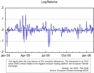
This figure plots the CO2 prices. The instrument is an ECX future 2006 contract traded at

the biggest emission trading platform: the European Climate Exchange.

(42)

30 May 2006 important because in case of non-stationary series, results of analyses of the price will be

misleading and for instance often have seemingly high R2_{scores. The presence of a unit root can}

help determine if the time series is indeed non-stationary. We can formally test for weak stationarity using the following equation, the Augmented Dickey Fuller test developed by Dickey and Fuller (1979):

The test is performed on the log of the prices with, based on the Akaike Info Criterion (AIC), zero lags specified. The table below shows the output of the test.