CSEIT411826 | Published - 25 April 2018 | March-April-2018 [ (4 ) 1 : 152-157 ]
National Conference on Recent Advances in Computer Science and IT (NCRACIT) International Journal of Scientific Research in Computer Science, Engineering and Information Technology
© 2018IJSRCSEIT | Volume 4 | Issue 1 | ISSN : 2456-3307
152
Person Identification by Lips using SGLDM and Support Vector
Machine.
Sameer Ahmad Mir
1, Qurat-ul-Ain
2, Sohrab Khan
3, Mustafa Ahmad Bhat
4,
Haider Mehraj
51,2,3,4Department of Electronics and Communication Engineering , BGSB University Rajouri J &k , India 5Assistant Professor,Department of Electronics and Communication Engineering, BGSB University Rajouri J &k, India [email protected], [email protected]2, [email protected]3, [email protected]4, [email protected]5
ABSTRACT
Biometric authentication techniques are more consistent and efficient than conventional authentication techniques and can be used in monitoring, transaction authentication, information retrieval, access control, forensics, etc. In many cases human identification biometric systems are motivated by real-life criminal and forensic applications. One of the most interesting emerging method of human identification, which originates from the criminal and forensic practice, is human lips recognition. In this paper we consider lips texture and color features in order to determine human identity. In our project, we are using Spatial Gray Level Dependence Method (SGLDM). For classification purpose, Support Vector Machine (SVM) will be used and for dimensional reduction Principal component Analysis (PCA) will be used. This quantative comparison is implemented through MATLAB. A standard XMV2TS database consisting sample images of seven persons is created. An analysis will be performed on all collected images and parameters will be compared to establish a working principle for person identification using lip recognition. The system will use threshold technique as identification tool.
Keywords : Biometric Authentication, SGLDM , SVM , PCA , Lip Recognition
I.
INTRODUCTION
Numerous measurements and signals have been proposed and investigated for use in biometric recognition systems .A biometric can be based on a person’s either physical or behavioral characteristics the most popular measurements are fingerprint, face and voice [1]. Each of these biometric traits has their own pros and cons with respect to accuracy and deployment. Among these features, face recognition is able to work at a greater distance between the prospective users and the camera than other types of features yet; one critical issue of the face recognition system is that the system cannot work well if the
machine [4]. The process of scanning and matching can occur through verification or identification. In verification, a one-to-one match takes place in which the user must claim an identity, and the biometric is then scanned and checked against the database. In identification, a user is not compelled to claim an identity; instead, the biometric is scanned and then matched against all the templates in the database. If a match is found, the person has been “identified.”
II.
METHODS AND ALGORITHMS
A. Local binary patterns (LBP)
Local binary pattern is a type of visual descriptor used for classification in computer vision [5]. LBP is the particular case of the Texture Spectrum model proposed in 1990. LBP was first described in 1994. It has since been found to be a powerful feature for texture classification; it has further been determined that when LBP is combined with the Histogram of oriented gradients (HOG) descriptor [6], it improves the detection performance considerably on some datasets. A comparison of several improvements of the original LBP in the field of background subtraction was made in 2015 by Silva et al[7]. The LBP feature vector, in its simplest form, is created in the following manner:
(1) Divide the examined window into cells (e.g. 16x16 pixels for each cell).
(2) For each pixel in a cell, compare the pixel to each of its 8 neighbors (on its left top, middle, left-bottom, right-top, etc.). Follow the pixels along a circle, i.e. clockwise or counter-clockwise.
(3) Where the center pixel's value is greater than the neighbor's value, write "0". Otherwise, write "1". This gives an 8-digit binary number (which is usually converted to decimal for convenience).
(4) Compute the histogram, over the cell, of the frequency of each "number" occurring (i.e., each combination of which pixels are smaller and which are greater than the center). This histogram can be seen as a 256-dimensional feature vector.
(5) Optionally normalize the histogram.
(6) Concatenate (normalized) histograms of all cells. This gives a feature vector for the entire window.
The feature vector can now be processed using the Support vector machine, extreme learning machines, or some other machine-learning algorithm to classify images. Such classifiers can be used for face recognition or texture analysis.
B. Spatial Gray Level Dependence Matrices
SGLDM is a statistical method, which consists in constructing co-occurrence matrices to reflect the spatial distribution of gray levels in the region of interest [8]. SGLDM is based on the estimation of the
second order conditional probability density g(i, j,d, Ө)[9]. This means that an element at location
(i,j) of the SGLD matrix signifies the probability that two different resolution cells which are in a specified orientation Ө from the horizontal and specified distance d from each other, will have gray level values i and j respectively[10]. The angle is used to evaluate the direction of texture, and the application of several distance values can provide a meaningful description of the size of the periodicity texture. Thus for different Ө and d values, different SGLD matrices result. The angle Ө is usually restricted to values of 0, 45, 90, and 135°, and the distance d is limited to values restricted to integral multiples of pixel size [11]. In our work, we are using SGLDM approach.
III.
FEATURE EXTRACTION
some statistical measures to extract textural characteristics from the GLCM. Some of these features are as follows
Contrast: It is a measure of the local variations of gray levels present in an image. Images with large neighboring gray level differences are associated with high contrast. This parameter can also characterize the dispersion of the matrix values from its main diagonal.
Contrast is defined as follows:
Where g(i,j) corresponds to the elements of co-occurrence matrix ,ie the probability of moving from a pixel with gray level I to a pixel with gray level j.
Homogeneity: This parameter, called also Inverse Difference Moment, measures the local homogeneity of an image. It assigns larger values to smaller gray level differences within pixel pairs. This parameter has opposite behavior of the contrast. More the texture has homogeneous regions, more the parameter is high. Homogeneity is written as
Energy: This parameter is a measure of image homogeneity; it reflects pixel -pair repetitions .Homogeneous images have very few dominant gray tone transitions, which result into higher energy[16]. Energy is defined as follows:
Entropy: The feature entropy is a measure of non-uniformity in the image or region of interest. If the image is heterogeneous, many elements on the co-occurrence matrix have small values, which imply
that entropy is very large. Entropy is inversely correlated to energy , it is given by the following expression:
Mean: The mean is determined by the homogenous brightness or darkness of the image. The more homogeneously bright the image is, the higher is its mean, and vice versa .The mean is written as:
Variance: It is a measurement of Heterogeneity and was correlated strongly with standard deviation.It characterizes the distribution of gray levels around the mean value calculated above. Therefore, variance increased when the gray levels values differed from their means. The expression of the variance is:
IV.SVM FOR CLASSIFICATION
distance between the two parallel hyperplanes. An assumption is made that the larger the margin or distance between these parallel hyperplanes the better the generalization error of the classifier will be . We consider data points of the form
{(x1,y1),(x2,y2),(x3,y3),(x4,y4)...,(xn, yn)}.
Where yn=1 / -1 , a constant denoting the class to which that point xn belongs. n = number of
sample. Each xn is p-dimensional real vector. The scaling is important to guard against variable (attributes) with larger varience. We can view this Training data , by means of the dividing (or seperating) hyperplane , which takes
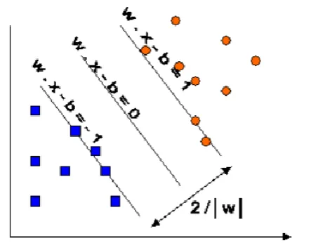
w . x + b = o --- (1)
Where b is scalar and w is p-dimensional Vector. The vector w points perpendicular to the separating hyperplanes. Adding the offset parameter b allows us to increase the margin. Absent of b, the hyperplanes is forsed to pass through the origin, restricting the solution. As we are interesting in the maximum margin, we are interested SVM and the parallel hyperplanes. Parallel hyperplanes can be described by equation
w.x + b = 1 w.x + b = -1
If the training data are linearly separable, we can select these hyperplanes so that there are no points between them and then try to maximize their distance. By geometry, We find the distance between the hyperplane is 2 / │w│. So we want to minimize │w│. To excite data points, we need to ensure that for all I either
w. x i– b ≥1 or w. xi– b ≤-1
This can be written as
yi( w. xi– b) ≥1 , 1 ≤i ≤n ---(2)
Figure 1. Maximum margin hyperplanes for a SVM trained with samples from two classes
Samples along the hyperplanes are called Support Vectors (SVs). A separating hyperplane with the largest margin defined by M = 2 / │w│that is specifies support vectors means training
data points closets to it. Which satisfy?
y j[wT. xj+ b] = 1 , i =1 ---(3)
(A) Model Selection For SVM
V.
EXPERIMENTAL RESULTS
Experiments are performed on gray level images to verify the proposed method. 8 bits per pixel represent these images. Face images are used for experiments are shown in below figure
Figure 2. Input Image Database
The next step is applying face detection on the above images. It is performed by the voila and jonne’s algorithm. The face-detected outputs are given below
Figure 3. Detected faces
Then the lip region is extracted from above images by taking some approximations. For eliminating the noise and camera influences suitable filtering is applied. Then the proposed features i.e contrast, energy, homogeneity, mean, variance and entropy are extracted and then each person is distinguished using support vector machine.
VI.CONCLUSION AND FUTURE WORK
Biometrics systems based on lip color and texture recognition are of great interest, but have received little attention in the scientific literature. This is perhaps due to the belief that they have little discriminative power. Thus, our experimental results show that by using spatial gray level dependence matrix algorithm along with support vector machine
we can recognize person based on his lips. In future, the work can be done on an identification system that incorporates the features of both lips and speech. Accuracy can be improved by the use of other feature extraction techniques. Accuracy can also be improvised by incorporating several feature extraction techniques to form a unique one.
VII.
REFERENCES
[1] Choraś, Michał. "The lip as a biometric." Pattern A nalysis and Applications 13.1 (2010): 105 - 112. [2] Lai-Kan-Thon, Olivier, "Lips Localization", Brno 2003.
[3] Tsuchihashi, Yasuo. "Studies on personal
identification by means of lip prints." Forensic Science 3 (1974): 233 -248.
[4] Chorás, Michal. "Emerging methods of biometrics
human identification. “Innovative Computing,
Information and Control, 2007. ICICIC'07. Second International Conference on. IEEE, 2007.
[5] X. Feng, M. Pietika inen, and A. Hadid, “Facial
Expression Recognition with Local Binary Patterns and Linear Programming,” Pattern Recognition and Image Analysis, vol. 15, no. 2, pp. 546-548, 2005.
[6] C.Shan, S.Gong, and P.W.McOwan, “Robust Facial
Expression Recognition Using Local Binary Patterns,” Proc. IEEE Int’l Conf. Image Processing, pp. II: 914-917, 2005.
[7] G. Zhang, X. Huang, S.Z. Li, Y. Wang, and X. Wu, “Boosting Local Binary Pattern (LBP)-Based Face Recognition,” Proc. Advances in Biometric Person Authentication, pp. 179-186, 2004
[8] Robert M.Haralick, K.Shanmugan, & Itshak Dinstein,
(1973) “Textural Features for Image Classification”, IEEE Transactions on Systems, Man and Cybernetics, Vol. SMC-3, No. 6, pp 610621.
[9] Andrea Baraldi & Parmiggiani Flavio, (1995) “An
Investigation of the Textural Characteristics
Associated with Gray Level Co-occurrence Matrix Statistical Parameters”, IEEE Transactions on Geoscience and Remote Sensing, Vol. 33, No. 2, pp 293-304.
[11]Mary M.Galloway, (1975) “Texture Analysis Using Gray Level Run Lengths”, Computer Graphics and Image Processing, Vol. 4, No. 2, pp 172-179.
[12]R.E. Haralick, K.Shanmugam, I.Dinstein, Textural
Features for Image Classification, IEEE
Transactionson Systems, Man and Cybernetics, Vol. SMC -3, No.6, Nov 1973
[13]Boser, B. E., I. Guyon, and V. Vapnik (1992). A training algorithm for optimal margin classifiers . In Proceedings of the Fifth Annual Workshop on Computational Learning Theory, pages. 144 -152. ACM
[14]V. Vapnik. The Nature of Statistical Learning Theory.
NY: Springer-Verlag. 1995.
[15]Chih-Wei Hsu, Chih-Chung Chang, and Chih- Jen
Lin. “A Practical Guide to Support Vector Classification”. Deptt of Computer Sci. National
Taiwan Uni, Taipei, 106, Taiwan
http://www.csie.ntu.edu.tw/~cjlin 2007
[16]C.-W. Hsu and C. J. Lin. A comparison of methods for
multi-class support vector machines. IEEE
Transactions on Neural Networks, 13(2):415-425, 2002.
[17]Chang, C.-C. and C. J. Lin (2001). LIBSVM: a library
for support vector
machines.http://www.csie.ntu.edu.tw/~cjlin/libsvm .
[18]Li Maokuan, Cheng Yusheng, Zhao Honghai