The entropy function for non polynomial problems and its applications for
Turing machines
Harvard Extension School [email protected]
MATHEUS SANTANA LIMA
We present a general process for the halting problem, valid regardless of the time and space computational complexity of the decision problem. It can be interpreted as the maximization of entropy for the utility function of a given Shannon-Kolmogorov-Bernoulli process. Applications to non-polynomials problems such as the Traveling Salesman Problem (TSP) are given. The new interpretation of information rate proposed in this work is a method that models the solution space boundaries of any decision problem (and non polynomial problems in general) as a communication channel by means of Information Theory. The limits of the search space are defined by the Kolmogorov-Chaitin complexity of the sequences encoded as Bernoulli strings. We conclude with a discussion about the implications for general decision problems in Turing machines.
Additional Key Words and Phrases: Computational Complexity, Information Theory, Machine Learning, Computational Statistics, Kolmogorov-Chaitin Complexity, Kelly criterion, Traveling Salesman Problem
ACM Reference Format:
Matheus Santana Lima. 2018. The entropy function for non polynomial problems and its applications for Turing machines. 1, 1 (March 2018),32pages.https://doi.org/10.1145/1122445.1122456
1 INTRODUCTION
Consider a Shanon-Bernoulli process P defined as a sequence of independent binary random variables X1, X2, X3 . . . Xn. For each element the value can be 0 or 1. All values have a given probability p. Thus the process is a sequence of independent and identically distributed Bernoulli trials. Let H(P) be the binary entropy function defined as the entropy of a Bernoulli process with probability p of one of two outcomes. A state is the representation (i.e. encoding) of a choice of the possible values for p. For any given trial there is no information about previous executions and future outcomes. Each execution of the process is stateless [21] [3]. Let a function g(X) be an indexing function. This function is a utility function used to represent a preference of ordering and is used to compare if alternative state A is preferable against alternative state B. If the probability density function for g(X) is an instance of a normal density function than the average of a given set of observations of a random variable - with finite mean and variance - is also a random variable that has a distribution that converges to a normal distribution as the number of samples increases. The entropy H(g(X)) for the function g(x) from a random variable X can not be greater than the entropy of the random variable X. Let Y=g(x). If the covariance of X and Y is not equal to zero than X and Y are correlated.
A Bernoulli scheme is a special case of a Markov chain and it’s a generalization of the Bernoulli process to more than two possible outcomes from an independent random variable. A Markov source is defined as a information source
Author’s address: Matheus Santana LimaHarvard Extension School [email protected].
Permission to make digital or hard copies of all or part of this work for personal or classroom use is granted without fee provided that copies are not made or distributed for profit or commercial advantage and that copies bear this notice and the full citation on the first page. Copyrights for components of this work owned by others than ACM must be honored. Abstracting with credit is permitted. To copy otherwise, or republish, to post on servers or to redistribute to lists, requires prior specific permission and/or a fee. Request permissions from [email protected].
© 2018 Association for Computing Machinery. Manuscript submitted to ACM
Manuscript submitted to ACM 1
created by a stationary finite Markov chain. The Kolmogorov complexity of a string is the length of the shortest computer program executed by a Turing Machine that produces the sequence as output and halts. It’s the measurement of the computational resources required to define this string. It can be proved that the Kolmogorov complexity of any string can not be larger than the expected length of the Bernoulli sequence itself. The entropy of the Markov information source is related to the Kolmogorov complexity. From "Kolmogorov complexity" in Wikipedia [27] [14]: "the Kolmogorov complexity of the output of a Markov information source, normalized by the length of the output, converges almost surely (as the length of the output goes to infinity) to the entropy of the source."
LetE(Y)be the expectation of the H(Y). A bit of information is the amount of entropy encoded in an event with two possible outcomes and even odds. The mutual information between two random variables X and Y can be used to optimize the growth of the utility function g(X) over many trials/executions. This is the "information gain" of a probability distribution for X given the value of Y relative to a given predefined a priori distribution (like the normal distribution) - or stated probabilities - on random variable X. LetK(E(Y),H(Y))be the maximization of the expected value of the logarithm of the entropy of the utility function Y, which is equivalent to maximize the expected geometric growth [26]. This fraction is the level of uncertainty between current and future states of X relative to E(Y). In other words this value represents the intensity of the “side information” measured from each element of the Bernoulli sequence. A program executing in any Universal Turing Machine can use this information to reduce entropy by adjusting the error rate in the long run. At each iteration the program must evaluate the level of uncertainty and decide if to halt or not. This implications contradicts the standard definition of the halting problem in which it proves that there is no general algorithm to solve the halting problem for all possible program-input pairs. The problem is in determining from an arbitrary description of an arbitrary program and an input whether the program will halt or run forever.
By analyzing the entropy of the logarithm of the utility function g(X) relative to the probability density function of a random variable X we can extract useful information about the overall distribution of possible output values in a given sample. Any programpncan use this knowledge to determine whatever programs halt for a given subset of program-input pairs symbols.
2 THESIS STATEMENT
The statistical analysis of the entropy function of H(Y=g(X)) and its correlation with random variable X can be used by any programpnto decide the limits in which cases the near-optimal values satisfy the halting condition. This decision must have statistical significance (under a given degree of freedom) and reduce the uncertainty about the possible states of values from random variable Y. In section 3.1 we describe the normal distribution function and the Shapiro-Wilk test of normality. In section 3.2 we describe the Shannon entropy function for Bernoulli sequences. In section 3.3 we discuss the optimization of the logarithm of the utility function of a random independent variable using the Kelly criterion and the Chi-square distribution. In section 3.4 we present the Indexing binary function for classification of states in decision problems. In section 3.5 we present an information theory interpretation applied to non polynomial problems such as the Traveling Salesman Problem. In section 4 we discuss previous works and background information on the TSP problem. In section 4.1 we present the TSP modeling using Information Theory and the stochastic algorithm. The conclusion summarizes the discussion and the implications for the computational limits of Turing Machines for a finite alphabet with a given mean and variance.
3 METHODS AND BACKGROUND
3.1 Sufficient Statistic
3.1.1 Normal distribution.The normal distribution (or the normal density function) is a continuous probability distribution for a random variable. The parameter value are the mean (or expected value) of a given real number and the standard deviation. The domain is (-∞,+∞). Its defined by the formula show in figure1:
Fig. 1. Formula for the normal distribution
From "Calculus Applied to Probability and Statistics" [19] the properties of the Gaussian-normal curve are defined in figure2:
Fig. 2. Properties of the normal distribution
Consider the functionд(Xn)=cn. The output for this function are the cost values c calculated from the input random sequences in{Xn}, with n finite and positive. The sequences are the semantic valid programs encoded by Bernoulli strings using a Shannon-Fano code. A Turing Machine executing these programs must decide if to halt by interpreting the random signals read from the tape. If the signal is statistically significant and the entropy is reduced then the program can stop and return the decision in binary representation. The computational complexity to decide the problem is additive to the machine implementing the program up to a limiting point.
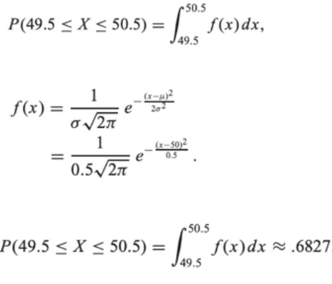
As an example let{p1,p2,p3}be a given set of programs and let the costs forд(X =001=p1)=c1,д(X =111=
p2) =c2,д(X =101 =p3)=c3. Let the acceptance threshold T for the machine M returns False when g(X) is off by more than 1%. Assuming that the cost values{c1,c2,c3}is a normal random variable with mean 50 and standard deviation 0.5. The range for the programs in this domain are 49.5<=д(X)<=50.5. The probability that a program will be accepted isP(49.5<=X <=50.5). Let f=g(X) be a normal random variable with median m= 50 and standard
deviation SD =0.5. Therefore from [19] we can see that 68.27% of the programs will be accepted and the remaining 31.73% will be rejected. The calculations are shown in figure3:
Fig. 3. Probability forP(49.5<=X <=50.5)
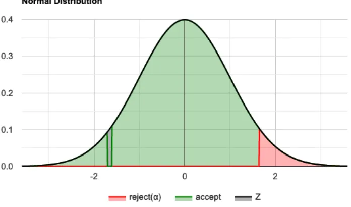
The normal distribution for Y=g(X) with mean = 50 and SD = 0.5 is shown in figure4:
Fig. 4. The normal distribution ofP(49.5<=X <=50.5)for g(X) with mean = 0.5 and SD = 0.5
3.1.2 Normality test.To determine if a data-set can be modeled as a normal distribution we can use the Shapiro-Wilk method to test the null hypothesis that the sample means came from a normal distributed population. In figure5its defined as:
Fig. 5. Shapiro-Wilk formula
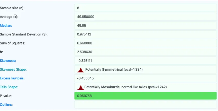
As an example, consider the cost samples fromд(X)={50,51,49,49.3,50.5,50.3,49.1,48}and a significance level of $alpha=0.05. The sample size, average and standard deviation are show in the figure6:
Fig. 6. The data distribution and p-value from the Shapiro-Wilk test for the function g(X).
Since the p-value>$alphawe accepted the H0 and we can assume the data is normally distributed. The distribution and the histogram are reproduced in figure7and8:
Fig. 7. The normal distribution for function g(X).
Fig. 8. The probability density function for function g(X).
3.1.3 Chi-square test. The Chi-square test can be used to determine whether there is a significant difference between expected and observed frequencies in one or more categories. The observations are classified into mutually exclusive classes according to a hypothesis described by the probability of observation of a value in each corresponding class.
The 2x2 contingency table for the chi-square can be used to compare two groups of dichotomous dependent variables. The formula for the Chi-Square test is defined in figure9:
Fig. 9. Chi-square test formula
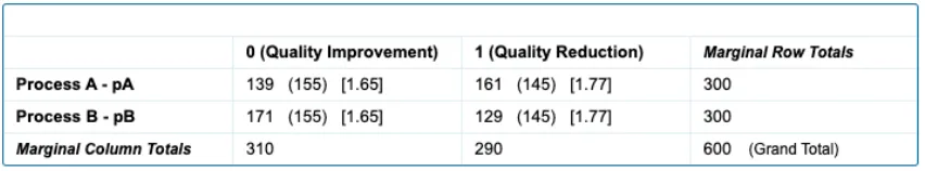
As an example consider two programs pA and pB that encodes 600 Bernoulli strings. Each program has a set of Bernoulli sequences that were classified between two groups: 0 and 1. Group 0 is the set with sequences with better costs than a given threshold (i.e. improves expected quality) and the group 1 is the sample-set with sequences with worse or equal quality (i.e. reduces or does not change the expected quality of g(X)). A chi-square test can be used to determine whether there is a significant difference between the proportion of sequences in programs pA and pB. The Contingency Table is show in figure10.
Fig. 10. Contingency Table for the expected value ofд(X)relative to random variable X.
The chi-square statistics is 6.8343. The p-value is .008943. There is enough evidence to reject the null hypothesis as p-value is less than $alpha = 0.05.
3.2 Information Theory
3.2.1 Entropy of a random sequence.Entropy is a measure of uncertainty of a random variable. In other words it’s the average rate at which information is produced by a stochastic process. Shannon defined the entropy H as a discrete random variable X with possible values as outcomes draw from a probability density function P(X) [21]. In figure11the entropy function is defined as:
Fig. 11. Shannon Entropy formula
The conditional entropy of two eventsX =xandY =ywithX =xiandY =yj for (i,j) andp(xi,yj)is the amount of randomness in the random variable X given Y. In figure12this relationship is defined as:
Fig. 12. Conditional entropy
Let consider for example a binary program p1 with probability p=0.7 for halting and returning True (state A) and 1-q for returning False (state B). At every trial one state is more likely to come up than the other. The reduction in entropy is expressed in a lower entropy value. The entropy for p!=q with p=0.7 is demonstrated in figure13:
Fig. 13. Entropy for p=0.7
3.2.2 Bernoulli distribution and the probability of success.If a random process can only have one of two possible outcomes (Success (True) and Failure (False)) with probabilities p and 1-q respectively than we have a Bernoulli trial. Let X be a random variable with X=1 for the "success" state outcome and X=0 for the "failure" state. The indexing function for event{X =1}is defined asI{Xk=1}=1 if X=1 andI{Xk =1}=0 if X=0 than X is a random Bernoulli variable with probability distribution defined as:px(Xk)=p×I{X =1}+q× [1−I{X =1}]andpx(Xk)=0 otherwise. The
median (expected value) and the variance Var[X] of the Bernoulli variable are defined by E(X) = p and the Var[X] = pq = p(1-p).
Consider for example a Bernoulli trial with size n for random variable X. Let g(x) be the utility function for X and p be the probability of a programpn producing as output a string which optimizes g(X). LetKc(X)be the length of the shortest program that outputs X and halts. Let H(X) and H(g(X)) be the entropy function for variable X and the function g(X) respectively. The only possible results are the event of interest F (i.e. finding the optimal solution to a given decision problem and thus maximizing the utility function) and event !F (i.e. not finding the optimal solution) with probabilities p=0.003 and q = 1-p = 0.997. The probability function for this Bernoulli trial is
px(Xk)=(0.003) ×I{X =1}+0.997× [1−I{X =1}]and 0 otherwise. For event F (Success state) let I[X=1] be the indexing function for value 1 and 0 when the outcome is event !F(Failure state). The median m and variance are m=0.003 and Var[X] = (0.003)(0.997) = 0.003.
3.2.3 Random variables and utility function.Let X be an independent random variable with alphabetL:{001,010,100. . .}. The utility function Y=g(X) of a random variable X express the preference of a given order of possible values of X. This order can be a logical evaluation of the value against a given threshold or constant. As an example ifд(X1=001)=c1 andд(X2=010)=c2 are the costs of two routes between a set of nodes - in a super-graph G* - we can use this function to determine the arithmetical relationship between them and decide if c1 is less, greater or equal to c2. The probability density function pdf(Y) can be used to calculate the entropy of the distribution of the cost values.
3.2.4 Entropy of the utility function.Let g(X) be a utility function of a random independent variable X with entropy H(g(X)). We need to determine the condition in which the entropy of function g(X) is not greater or equal than the entropy of X. This relationship is defined byH(д(X))<=H(X). From Wiegand and Schwarz [25] we have the proof of this condition:
3.2.5 Kolmogorov Complexity.The Kolmogorov complexity of a string w from language L denoted byKL(w)is the shortest program from alphabet L which produces w as output and halts. [14] The conditional Kolmogorov complexity of string x relative to word w is defined byKL(w|x)and is the length of the shortest program that receives x as input and produces w as output.
3.2.6 Complexity of a string and shortest description length.LetUbe a Universal computer. The Kolmogorov complexity
Kc(x)of a string x of a computerUis
Kc(x)=minlenдth(p)
when
p:U(p)=x
It is the minimum length programpthat output variable x and halts. Its the small possible program. LetCbe another computer. If this complexity is general there is a universal computerUthat simulatesCfor any string x by a constant con computerC. ThusKc(x)U <=Kc(x)C+c. This constant does not depend on string x. The upper bound on the Kolmogorov complexity is
Kc(x)<=Kc(x|lenдth(x))+2 log2lenдth(x)+c
Therefore there are few sequences with low complexity in the set. The lower bound states that are not many short programs in the set. If X is a Bernoulli sequence with probabilityp(x)=1/2, this means there are no more than 2k strings with complexityKc(x)<k.
Consider each program can produce only one possible output, the number of sequence with complexityKc(x)<kis less than 2k. Thus the complexity will depend on the computer up to an additive constant. Lets consider fractals for example. They can produce complex 2d images with self-replicating patterns with many different scales. However the complexity to describe its rules have a Kolmogorov Complexity close to zero. [3]
The expected value of the Kolmogorov complexity of a random sequence is close to the Shannon entropy. This relationship between complexity and entropy can be described as a stochastic process drawn to a i.i.d on variable X following a probability mass function p(x). The symbol x in variable X is defined by an finite alphabet. This expectation is
E(1/n)Kc(Xn|n)=>H(X)
Therefore most of the sequences in the set do not have simple description. However there are some simple sequences. The probability that a random sequence can be compressed by more thankbits is no greater than 2(−k). Thus most Bernoulli sequences have a complexity close to their length.
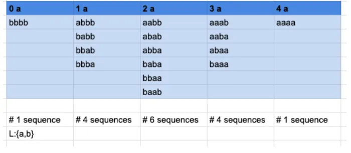
Let a binary sequence S from alphabetL:{a,b}with four characters (length n=4). Let the program p be any sort algorithm using as primary keys k1. This key is the number of occurrence of the symbolain string S. Let E(S) be the expected value of the distribution of S. The function g(S, E(S)) is the utility function which evaluate the relationship between the elements of a random string and a given cost function. The probability density function pdf of the utility function and the distribution of symbols in the sequence are defined by pdf(g(S,E(S))=Y and pdf(S)=Z respectively. The entropy function are defined for Y and Z. The search space for the program p is show in figure14:
Fig. 14. Search Space distribution
Let P(A) = P(sequence with a pair of a) withP(A) = {bbbb,aabb,abab,abba,baba,bbaa,baab,aaaa}. Let P(B) = P(sequence with 3 a). Let M = 4 be the favorable states to event B and N=16 are the total of possible outcomes. Than
P(B)=M/N =4/16=1/4.
The Kolmogorov complexity of a independent and identically distributed random binary variable created by a Bernoulli process is close to the entropy binary function. The expected value of the complexity of the Bernoulli sequence
converges to the entropy. Therefore we can bound the number of sequences with complexity that are significantly lower than entropy and classify each element between two sets(the typical sets and a non-typical set).
3.2.7 Kelly criterion and the uncertainty in random outcomes.LetK(E(Y),H(Y)) = f be the maximization of the expected value of the logarithm of the entropy of the utility function Y=g(X) [13]. This fraction is known as the Kelly criterion and can be understood as the level of uncertainty about a given data distribution of the random variable X relative to a probability density function pdf(Y) of a measured respective cost distribution found at the sample. The value of f is a fraction of the cost-value of g(X) on an outcome that occurs with probability p and odds b. Let the probability of finding a value which improves g(X) be p and in this case the resulting improvement is equal to 1 cost-unit plus the fraction f. The probability of decreasing quality for Y is 1-p. Therefore the expected value for log cost (E) is differed in figure15as:
Fig. 15. Expected value of the utility function
From "Kelly criterion" in Wikipedia [26], "To find the value of f for which the expectation value is maximized, denoted as f*, we differentiate the above expression and set this equal to zero.”. In figure16we have the maximization of the expected value.
Fig. 16. Maximization of E(X)
Where f* is the optimal fraction, b is the net odds, p is the probability of improving quality in Y=g(X) and the q is the probability of decreasing quality (1-q).
For example consider a program with a 60% chance of improving the utility function g(X) thus p=0.6 and q=0.4. The program has a 1-to-1 odds of finding a sequence which improves g(X) and thus b=1. For this parameters the program has a 20%(f*=0.20) of confidence that the outcomes produce values that improve the expected value of g(X) over many trials.
3.3 General Decision Machine
From Hopcroft & Ullman [11] a single-tape Turing Machine can be defined as a 7-TupleT M=<Q,Γ,b,Í,δ,q0,F >
where Q is a finite set of states,Γis a finite tape with symbols from a given alphabetL0,bis the blank symbol and
b ∈ Γ,Í⊆Γ− {b}
is the set of input symbols,q0 ∈Qis the initial state,F ∈Qis the set of final accepted states,
δ:Q−F×Γ−→Q−F×Γ×L,Ris a partial function called the transition function where L and R are the Left and Right shift respectively.
Let X be a random symbol from the alphabetL0. We can expand the standard Turing Machine model to a general computation under a given know distribution with probability p. Consider the utility functionд(X)related to the machine TM. The output of g(X) is dependent on the changes in the value of x in X. Assume that the values of g(x) follow a normal distribution. Let the probability density function of g(X) be pdf(g(X)). The entropy H from g(X) relative to X can be calculated. LetK(E(Y),H(Y)) =f∗be the maximization of the expected value of the logarithm of the entropy of the utility function Y=g(X).
3.4 Indexing binary function
Let theCp(X,д(X))be the p-value from the Chi-Square Test for random samples. Assume the samples are normally distributed. These functions evaluate whether the sample means are generated from the same distribution. Each element of the sample is a random independent variable X that is compared to the output of the utility function Y=g(X). This utility function is a conditional statement that returns(i.e. produces as a output) True or False by evaluating if a given x in g(X) is greater, small or equal to a given threshold defined as a real value T. Let E(Y) be the expected value of Y with entropy H(Y). The functionK(E(Y),H(Y))is the uncertainty level about the state distribution between the random samples. In other words, this value represents the error rate in the representation of information in a give population under some degrees of freedom. The function K is the maximization of the expected value of the logarithm of the utility function g(X) of a random variable X.
The domain for functionCp(X,д(X))is the range from 0 (no change) to 1 (high confidence). The value outputted by this function is the significance level. For example a value of 0.05 represents a 5% chance. The domain for function K is
(−∞,+∞). The K value represents the intensity about the uncertainty of randomly finding state outcomes that improves (or reduces) the utility function Y=g(X). If the K value is positive then it shows the amount of useful information encoded in the sample. For example if the value is 0.05 (5%) then the uncertainty is reduced (i.e decrease in entropy) and there is additional side information transmitted by the information source. If the edge is negative the K value is also negative indicating that the chance of finding useful information from the elements in the random sample is unlikely.
Let M be an index function that classifies a sample according to the distribution of elements in probability distribution of a function g(X). The classification labels each element in the sample between Accept/True or Reject/False. After the categorization of all input values the list of executions can be sorted by this label. In other words M is the sort key in a rank of sequences. The function M is defined byM=Cp(X,д(X))/K(E(Y),H(Y))
where X is a Bernoulli sequence, Y=g(X) is the utility function, H(Y) is the entropy for Y, K is the uncertainty level, E(Y) the expected value of Y. The domain is(−∞,+∞).
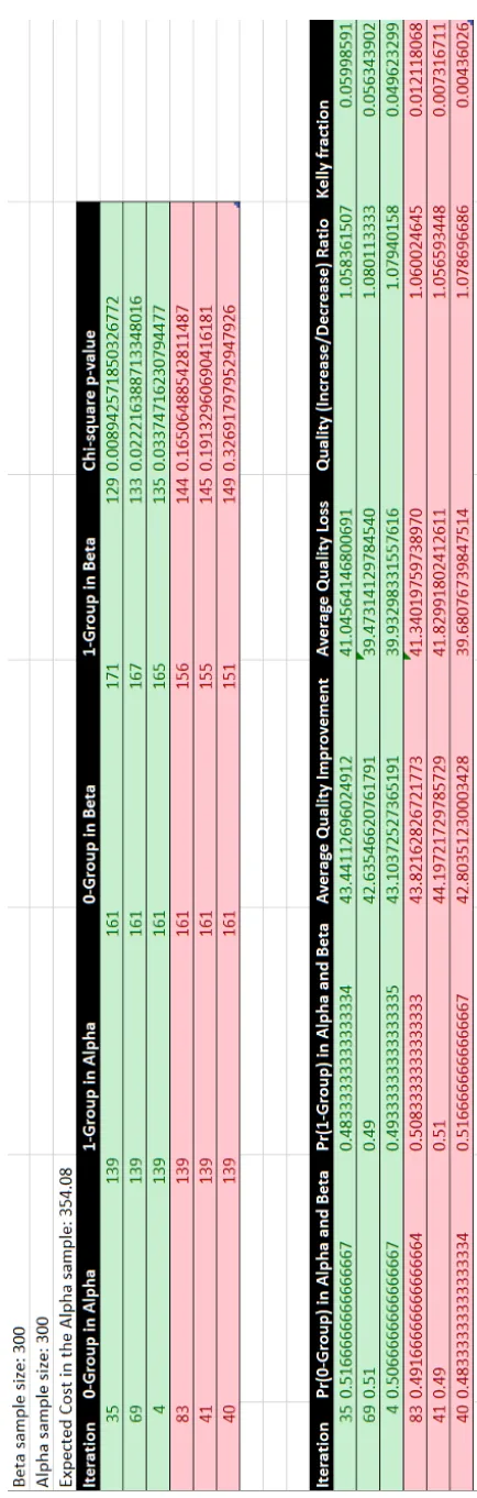
Let’s consider for example two groups (alpha and beta) of random Bernoulli sequences for a trial of size 100. Both samples are assumed to be normal distributions. Letpbe a program that needs to decide to halt based on the expectation of the output values for the utility function g(X). The output domain is defined as the cost values of the elements in each group (encoded as random strings of X). The fixed alpha sample is the known model-reference set and the beta sample is the alternative sample hypothesis. Both samples have 300 candidate solution sequences each(N=600). The computed executions with chi-square p-value less than 0.05 and Kelly fraction greater than 0 are the solutions of interest and they produce greater quality by reducing entropy at each interaction. Let’s consider the subset s* of sequences produced at interactions∗={35,69,4,83,41,40}. We want to classify each element of s* between two categorical classes: the near
optimal sequence pools (interaction 35, 69 and 4) and another random sample with discarded sequence samples (83, 41, 40). In the figure below, we can see the p-values and Kelly fractions for instance 4, 35, 69 (good near optimal solutions) and 41, 40 and 83 (random bad solutions). We want to filter solution sequences with candidate solutions that produce significant results and have a maximum rate of decrease in entropy. In other words, there is less uncertainty about the possible favorable state outcomes - relative to g(X) and E(Y)- with the new alternative sample against the previous known best solution hypothesis set. In the figure17we have the representation of the probability density function, the p-value for the Chi-square test and the Kelly fraction relative to the measured level of uncertainty.
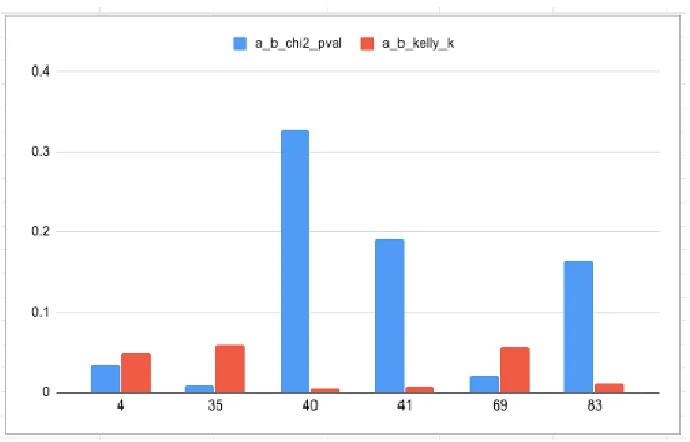
By comparing the p-value and the Kelly fraction any programpn can decide whatever to halt based on “side information” on which symbols can lead - in the long run - to the best possible rate of quality improvement for the utility function g(X), over finite many interactions. Therefore the halting problem is reduced to a sort problem using the p-value and the Kelly fraction as the primary and secondary keys for an unsorted computation list. To find the best near optimal sequence any program can sort the keys by decreasing order. Additionally it can sort the sub-list by the number of bits required to encode the binary - near optimal - string in a Shannon-Fano code following the probability density function pdf(g(X)). The relationship between the p-value and the kelly fraction is show in figure18:
Fig. 18. Bar chart for the p-value from the Chi-square test and the Kelly fraction
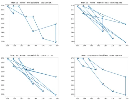
In the figure19we can see the maximum and minimum cost distance from A and B at interaction 35.
Fig. 19. Minimal and maximal path cost
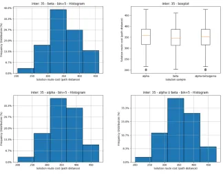
In the figure below we can see the histogram for the cost distance from both samples grouped by a bin of size 5 for inter 35. We can see there are a larger concentration in group A (alpha) of solutions with cost between 350 and 450 than in group B(beta). From the boxplot20shown we know that although it’s an outlier there are candidate solutions in group A with cost distance at around 200 units. On the other hand in the group B the average distance is smaller 348.738 units and more spread than in group A 354.08 units. It’s important to note that the information about the local minimal distance close to 200 was already in A. However, there are more elements with cost close to the minimum distance of 200 in B than in A.
Fig. 20. Histogram and Boxplot for Alpha and Beta sets
3.5 Applications
The indexing binary function M can be used as a key to decide if a given decision problem should halt or not. For example the Traveling Salesman Problem (TSP) wants to find the shortest route in a graph of connected nodes. Another example is the game of Sudoku where the candidate solution that has a better partial solution has a better score than other alternatives. The Sudoku puzzles is a grid of partially completed rows and cells partitioned in regions. A solution using distinct symbols from alphabet L such that row, column and region have exactly one of each element of the set. The general problem of Sudoku is NP-complete.
The function M can label each output and decide whether to halt if the intensity of M is above a given threshold T. In other words the state of any Bernoulli sequence has a proportional real value that ranges according to the variation in entropy of the utility function of the candidate strings. Both Sudoku and the TSP are in the class of non-polynomial (NP) class of problems [28].
In this paper we have proposed a new approach for uncertainty modeling based on the Kelly-Shannon-Thorp [23] [21] [13] criterion to measure the optimal channel allocation that a program should place at each interaction of an algorithm (implemented in a Turing Machine) for solving any non polynomial decision problem such as the Traveling Salesman Problem. This new interpretation of the NP problems by means of Information Theory and Kolmogorov-Chaitin Complexity can be used to define the limits of computation and answer the question of which cases P=NP. It works by setting the boundaries of the problem as a probability density function draw according to a sample of random solution samples defined as semantic valid Bernoulli binary strings. Each candidate solution cost is evaluated against a binary statistical indexing function M in order to classify it between 2 independent groups: 0 (smaller cost — better quality);
1 (greater or equal cost — worse or unchanged quality). This distribution reveals the amount of inside information available to the program and the entropy can be calculated. The Turing Machine can then use this information to reduce entropy at each execution clock unit while maximizing the expected improvement in solution quality (ie finding a shortest euclidean distance tour that visits all nodes as described in the TSP problem). In the TSP, the salesman receives a list of cities and paths from a “wire” or “tape” and must decide between accepting any given new route against the current know best route. If he is lucky and chooses the right path, he may very well end with a smaller distance to travel across all cities and returning home. If he chooses the wrong path he may end up with thinking the current total distance is the best one even though it’s not. For the classical salesman there is no way to know how good or bad his path is because he has no inside information about the overall expected distance of the routes. At each execution clock he must decide using only his current knowledge for that iteration about the best distance so far and the new alternative solution.
Alternatively, the log-normal salesman’s can improve his strategy in the long run by quantifying the total of available inside information in the channel (or a tape in the Turing machine) and maximizing the expected value of the logarithm of value function (defined by Traveled Euclidean distance) for each execution clock. Using this approach, he can reduce his uncertainty while optimizing his rate of distance reduction (quality improvement) at each execution time. He can do it by creating the probability density function of the cost distance variable by sampling two sets (current and new) of random tours distances.
4 PREVIOUS WORK & PRELIMINARES
This section contain an overview of the most important heuristics to solve the TSP problem. Other algorithms such as Nearest Neighbor, Greedy, Insertion, Christofides, Lik-Kerninghan, Branch & Bound and Ant Colony Optimization were not discussed in this paper. Those methods and its complexity considerations is studied in details by Nilson [20].
4.1 Heuristics for the TSP & Graph Theory
An algorithm that is searching for the smallest distance (cost or weight) between nodesvanduin a graphGmust record the information about the intermediary distances tow. This information can be encoded as a label attached to the nodes where its value is defined as the distance between v and w. [5] For n nodes We can use an distance matrix
D=(di,j)nxn
where each element represents the distance between each city-nodes. LetsΠbe the set that contains all possible permutations from node 1 to n. Zhan et al[29] in his work described that the goal of the TSP is to find a permutationπ that minimizes the distance between nodes. For symmetric instances the distance between two nodes in the graph is the same in each direction, forming an undirected graph. For asymmetric instances the weights for the edges between nodes can be dynamic or non-existent.
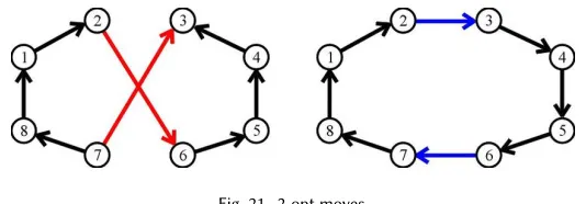
4.1.1 2opt, k-opt.Croes [4] proposed the 2-opt algorithm, an simple local-search heuristic, to solve the optimization problem for the TSP. It works by removing two edges from the tour and reconnects the two paths created. The new path is a valid tour since there is only one way to reconnect the paths. [20] The algorithm continues removing and reconnecting until no further improvements can be found. k-opt implementations are instances of 2-opt function but withk>2 and can lead to small improvements in solution quality. However as k increases so does the time to complete execution.
In his work Glover [8] proposed the Tabu Search method and it can be used to improve the performance of several local-search heuristics such as 2opt. As neighborhood searches algorithms like 2opt can sometimes converge to a local optimum, the Tabu search keeps a list of illegal moves to prevent solutions that provide negative gain to be chosen frequently. In 2opt the two edges removed are inserted in the tabu list. If the same pair of edges are created again by the 2opt move, they are considered tabu. The pair is keep in the list until its pruned or it improves the best tour. [20] However using tabu searches increases computational complexity toO(n3), as additional computation is required to insert and evaluate the elements in the list.
The Figure21show the 2-opt moves from Zunic et. al [31].
Fig. 21. 2-opt moves.
Nilsson [20] compared several heuristic strategies for the TSP problem such as Greedy, Insertion, SA, GA, etc. He investigated the performance trade off between solution quality and computational time. He classify the heuristics in two class: Tour construction algorithms and Tour Improvement algorithms. All algorithms in the first group stops when a solution is found. In the second group, after a solution is found by some heuristics, it tries to improve that solution (up to certain computation and/or time constraints.)* He concluded by showing that the computational time required is proportional to the desired solution quality.
4.1.2 Genetic Algorithm (GA). Genetic Algorithms was first introduced by Hollad [9]based on natural selection theory, as an stochastic optimization method in random searches for good (near-optimal) solutions. This approach is analogous to the "survival of the fittest" principle presented by Darwin. This means that individuals that are fitter to the environment are more likely to survive and pass their genetic information features to the next generation.
In TSP the chromosome that models a solution is represented by a "path" in the graph between cities. GA has thee basic operations: Selection, Crossover and Mutation. In the Selection method the candidate individuals are chosen for the production of the next generation by following some fittest function In the TSP This function can be defined as the length (weight) of the candidate solutions tour. In figure22we have a representation of genes and Chromosomes.
Fig. 22. Chromosome for a sample of individual candidate solutions..
Next those individuals are chosen to mate (reproduction) to produce the new offspring. Individuals that produce better solutions are more fit and therefore have more chances of having offspring. However individuals that produces worst solutions should not be discarded since they have a probability to improve solution in the future. In other words, the heuristic accepts solutions with negative gain hopping that eventually it may lead to a better solution.
Several researches have studied the performance trade off of selection strategy and how the input parameters affects the quality of solution and the computational time. Julston studied the performance of rank-based and concluded that tournament selection presents better results than rank-based selections.[18] Razali et al. [18] in his work explores different selection strategies to solve the TSP and compare the performances quality and the number of generations required. It concludes that tournament selection is more appropriate for small instance problems and rank-based roulette wheel can be used to solve large size problems.
Goldenberg & Deb [6] compared the quality of the solution and the convergence time on many selection methods such as proportional, tournament and raking. They conclude that ranking and tournament have produced better results that proportional selection, under certain conditions to convergence. [18] In his work Zhong et al. [30] explored proportional roulette wheel and tournament. He concluded tournament selection is more efficient than proportional roulette selection.
The figure23contains the pseudo-code for a Genetic Algorithm from Ferentinos et. al [7]
Fig. 23. Basic genetic algorithm.
4.1.3 Simulated Annealing (SA).Simulated Annealing are heuristics with explicit rules to avoid local minimal. It can be described as a local random search that temporarily accepts moves with negative gain( i.e were produced by solutions with worst quality than current). This methods simulates the behavior of the cooling process of metals into a minimum energy crystalline structure. This concept is analogous to the search of global maximum and minimum. The probability of accepting a solution is set by a probability function of a temperature parameter variable. As the temperature decreases over time the probability change accordingly. The acceptance probability is defined asp(x)=1 iff(y)<=f(x)and when otherwise
p(x)=e[−(f(y)−f(x))/tmp]
wheretmpis the input temperature. The SA algorithm specifies the neighborhood structure and the cooling function. From Chien et. al [2] we can see the flow chart in figure24for the Simulated Annealing algorithm:
Fig. 24. Simulated Annealing
Other heuristics such as 2-opt, 3-opt, inverse, swap methods can be use to generate candidate solutions. Several researches have been made to study the performance of different SA operators to solve the TSP problem. [1][12][10][24] Zhan et. al [29] proposed a list-based SA algorithm using a list-based cooling method to dynamically adjust the temperature decreasing rate. This adaptive approach is more robust to changes in the input parameters. In his work Chien et. al [2] proposed a genetic simulated annealing inspired by ant colony systems. They conclude that the average solution results are better than the traditional SA and GA methods alone.
The quality of the solution can be improved by allowing more time for the algorithm to run. Steiglitz and Weiner [22] observed that the performance of 2-opt and 3-opt algorithms can be improved by keeping a ordered list of the closest neighbors for each city-node and thus reducing the amount of solutions to search.
4.1.4 Nature inspired models.Researchers have proposed algorithms inspired by natural events and structures like the heating of metals and the growing behavior of biological organisms. Those methods do not iterate over the entire solution space but rather a portion in order to find the local minimum. They start with an initial random solution and tries to improve the solution quality over each interaction until some constant parameter factor is reached like a maximum number of interactions, maximum number of candidate solutions, the rate of decay in temperature or a minimum quality threshold is achieved. This can be interpreted as a non-deterministic way to address the error rate between the known solutions and the unknown solutions in polynomial time. Although such algorithms do not have to traverse the entire solution space it must decide when a random candidate solution with negative gain will be accepted (i.e. candidate with worst solution quality than current know best solution) in the hopes that eventually it would lead to the shortest distance (i.e. a better solution quality).
What those methods have in common is that they ignore the data distribution of input and output strings for the candidate solutions sequences. The algorithm does not care which city it starts and ends the tour, as long as the solution sequence is semantically valid it must decide whether to return true or false using some function that defines the decision rules based on the current best known total Euclidean distance tour. At each interaction those heuristics are trying to optimize the calculated value function set as the total tour distance for that specific trial, it has no information
about the other possible candidate solution strings in the solution space. This assumption introduces a bias in the algorithm since it implicitly assumes a prior knowledge about the data structure in order to reduce the resources required to complete the computation. Put it simply, the algorithm is never sure if the solution at hand is the optimal and may very well discard it hoping to look for a better one in the future based on some arbitrary criteria.
In the TSP problem all non-deterministic algorithm will have to work with random input and output sequences and for each one it must decide when to halt or not. The candidate tour sequences from the perspective of the Turing machine are random symbols being read by the machine’s head. All the available inside information are the symbols in the tape. The tape is the communication channel used to transmit the messages (i.e. candidate solutions). Therefore, modelling the TSP by means of Information Theory and Kolmogorov Complexity is the natural language as the number of possible candidate solutions are very large even for small instances of the problem. This means that all cities are assumed to have the same probability of being chosen and the outputted total tour distance would be proportional to this choice over many trials.
Nature-inspired models such as GA and SA uses prior information to improve the solution results and thus are biased towards this encoding. Alternatively, by modeling the TSP problem as a communication channel with a probability density function associated with the stochastic process that generates the solutions at random, thus we can bound the limits of the search space to a log-normal distribution. The advantage of this method is that by relying on the statistical analysis of the solution space instead of the computational complexity of the problem we can have equal or better qualities than the traditional algorithms without relying on computational complex implementations that have a high time and space constrains.
5 ALGORITHMIC-INFORMATION LANGUAGE
Let L be a finite language with N symbols in a set such asL: {NODEA;NODEB;NODEC, . . .NODEN}. Each item is an identification label for the elements in the set under some probability distribution function pdf(x). This is the likelihood of choosing a given symbol x in L. This can be interpreted as a random variable x in L that can assume any item in the set by following the known distribution pdf(x). Each symbol represents a city with a 1–1 mapping to a respective node in a super-graph G*. Therefore, each node is a point withXnandYncoordinates in a 2D Euclidean space. Let the function g(X) be the utility function for a given language L. This functions outputs the costs or weight of X relative to a given threshold T defined as the expected value of E(g(X)). Assume g(X) is a Bernoulli distribution.
For example consider the alphabet L that describes 3 cities encoded by 3 symbols in the setL:{A(x1,y1),B(x2,y2),C(x3,y3)}. Thus, each element is a node that have two variables that stores the x and y axis coordinate accordingly. A valid sequence s* can be produced by combining elements of L. Permutations with duplicate elements are invalid. S* is the set with all possible permutations of this sequence. The neighbor of each node at position i in the sequence is the next connected city (i.e item at position i+1). This sequence describes a path between nodes and is a tour starting from the first node until the last and returning to the first node when finished [15]. This is shown in figures25and26:
Fig. 25. Cost Matrix
In figure26we have an example of valid and invalid tours sequences:
Fig. 26. Sample path strings
In the figure27and28we can see an example of the probability density function for two random samples with N=4 for both sets: Group A and B. The new expected cost for the sample Group B is 49.25 units. For example if the expected cost for the current sample was 50 (in Group A) there are 2 solutions in B and 1 candidate in A which improve the solution quality and reduces the traveling distance. The probability of finding a candidate solution at random in group A that reduces cost is 25%. The probability of finding a candidate solution at random in group B that reduces cost relative to the expected cost distance from A is 50%.
Fig. 27. Group A candidate solution sample
The average quality improvement from B is 26.5 units with distance reduction from expected cost of 50 to 35 and 50 to 12. The average quality decrease or unchanged is 25 units, from 50 to 50 and 50 to 100. The rate of improvement is the average distance reduction divided by the average quality reduction. For this example, 26.5/25 = 1.06. In the figure 28we can see the data distribution for group B relative to the costs from E(A):
Fig. 28. Group B candidate solution sample
The Kelly criterion is 0.0283 (2.83%). This can be interpreted as a measurement of risk that a salesman has on choosing the wrong path (with larger distances). In simple terms, it’s the level of uncertainty about the overall possible states. This is the error rate of transmission of information in a noisy communication channel. If the fraction is negative the salesman must switch strategy and stay with current know best path sample and wait for the next alternative sample that will be created at the next execution iteration clock. [16].
Fig. 29. Kelly fraction to measure information uncertainty
The entropy of the new cost output is one full bit of information and is show in figure30
Fig. 30. Entropy for p =0.5 and q=0.5 with p = 1 — q
The contingency table for sample is demonstrated in figure31:
Fig. 31. Contingency Table for current (Group A) and alternative (Group B) solution candidates relative to expected current cost from Group A.
Consider for example a larger solution sample. The current solution group (A) and the alternative solution group (B). Group A has 100 solution sequences and B also has 100 candidates. There are 25 possible candidate tours that reduce the distance in A. In group B there are 50 candidates that increase the average cost relative to current expected distance from A. The salesman can use the chi-square test statistic to determine if there is a significant difference between the sample means. This can be used to determine if the expected distance decrease from the candidate solutions in group A (i.e. null hypothesis) is equivalent to the performance of the alternative candidates in group B (i.e. alternative hypothesis). The chi-square statistic and p-value are shown in the figure32
Fig. 32. Contingency Table for group A and B relative to E(A)
The chi-square statistic is 13.3333. The p-value is .000261. The result is significant atp< .05. With a significance level of 0.05 there is strong evidence against the null hypothesis and there is a 5% chance the null is correct. We can reject the null hypothesis and accept the alternative hypnosis that Group B has solutions that produce better quality than in Group A.
5.0.1 Algorithm and Pseudo code.In the figure33we can see the flowchart for the salesman stochastic algorithm:
Fig. 33. Flowchart for the information theory based algorithm
The pseudo-code for the procedure is described below:
A-Sample(Reference group): Create a model sample A using a random generated (semantic valid)
solution, 2-opt method, Simulated Annealing, Genetic Algorithms or any Artificial Intelligence
heuristics.
Let E(A) be the expected cost for the candidates in sample A.
Category(A,1): Count the number of candidate solutions in sample A that have total path
distance (ie cost value) greater or equal to E(A).
Category(A,0) : Count the number of candidate solutions in sample A that have total path
distance (ie cost value) less than E(A).
Pr(A,0): Calculate the probability of randomly finding a candidate solution in sample A that
increases quality (i.e. reduces cost).
Pr(A,1): Calculate the probability of randomly finding a candidate solution in sample A that
decreases quality (i.e. increase cost).
Let A_QualityIncrease: Average quality improvement for sample A.
Let A_QualityReduction: Average quality reduction for sample A.
Let R_Quality_A: A_QualityIncrease/A_QualityReduction be the ratio of quality in sample A.
Let Halt = False be the control boolean flag.
While Halt is equal to False, Repeat:
B-Sample: Create an alternative sample B using a random generated (semantic valid) solution,
2-opt method, Simulated Annealing, Genetic Algorithms or any Artificial Intelligence heuristics.
Category(B,1): Count the number of candidate solutions in sample B that have total path
distance (ie cost value) greater or equal to E(A).
Category(B,0) : Count the number of candidate solutions in sample B that have total path
distance (ie cost value) less than E(A).
Pr(B,0): Calculate the probability of randomly finding a candidate solution in sample B that
increases quality (i.e. reduces cost).
Pr(B,1): Calculate the probability of randomly finding a candidate solution in sample B that
decreases quality (i.e. increase cost).
Let B_QualityIncrease: Average quality improvement for sample B.
Let B_QualityReduction: Average quality reduction for sample B.
Let R_Quality_B: B_QualityIncrease/B_QualityReduction be the ratio of quality in sample B.
CT_AB: Create the Contingency Table for groups A and B with the occurrences of each 10
Categories.
Chi2_AB: Calculate the Chi-square test for CT_AB.
k_AB: Calculate the Kelly fraction for Pr(A+B,0) and R_Quality_A + R_Quality_B.
info_B: Calculate the entropy for the estimated probability distribution function from
alternative sample B using CT_AB.
if Chi2_AB < 0.05 and k_AB > 0 than return [Halt=True, “Solution Found.”] else [Halt=False,
“We don’t have enough evidence and/or information to reject the null hypothesis]
6 CONCLUSION
In this paper we have demonstrated the statistical analysis of a stochastic process created by a set of Shannon-Bernoulli sequences. From this framework it’s possible to analyze the distribution of information for a given random variable and the correlation between this variable and a utility function that compares the differences between state sequences. This function shares information with the random variable itself and this side information can be measured. The knowledge of this side information can be used by any program - executing in a Turing Machine - to decide whatever to halt or not. This model can be used to optimize the performance of heuristics algorithms such as Simulated Annealing, Genetic Algorithms and 2-opt applied to the Traveling Salesman Problem (TSP). The advantage of this approach is that it is independent of the computer encoding the problem and the time and space complexities are additive up to a limit that is linearly proportional to the input size. Other heuristics methods assume a predefined knowledge about the data structure and thus are biased towards this encoded knowledge. The implications of this interpretation is that by reducing the NP problems to a matter of modularization of encoded and decoded random signals in an alphabet we can find near optimal solutions that are statistically significant and are guaranteed to produce the best rate of improvement in the long run over many trials(i.e. simulation iterations) even though the problems itself is computationally complex and the alternative sequential brute force algorithm would require exponential time to solve.
From Fekete et al. [17] the classical interpretation of hard decision problems argues that unless P=NP there is no polynomial-time algorithm for NP problems such as the TSP: "Assuming triangle inequality, the best polynomial heuristic known to date uses the computation of an optimal weighted matching: Christofides method combines a Minimum Weight Spanning Tree (MWST) with a Minimum Weight Perfect Matching of the odd degree vertices, yielding a worst-case performance of 50% above the optimum." The traditional interpretation of the halting problems says there is no general algorithm to solve the decision problem for all possible program-input pairs. However, as demonstrated
in this paper, the decision problem itself can be quantified in bits and the distribution of random sequences that are -syntactically and semantically - valid is not neglectable. In other words, although not all sequences produce outputs that optimizes the quality for any utility function g(X), there are some infrequent random sequences that improve g(X) and are statistically significant under some given degree of freedom. This new interpretation of information rate can be used to define the limitations imposed by the computational complexity of Turing Machines when solving non polynomial problems, regardless of time and space constraints.
REFERENCES
[1] E. H. Aarts, J. H. Korst, and P. J. van Laarhoven. 1988. A quantitative analysis of the simulated annealing algorithm: a case study for the traveling salesman problem.Journal of Statistical Physics, vol. 50, no. 1-2, pp. 187–206(1988).
[2] Shyi-Ming Chen and Chih-Yao Chien. 2011. Solving the traveling salesman problem based on the genetic simulated annealing ant colony system with particle swarm optimization techniques.Expert Systems with Applications. Elsevier.Volume 38, Issue 12, November–December 2011, Pages 14439-14450 (2011).
[3] Thomas M Cover. 2012. Elements of information theory.John Wiley Sons(2012).
[4] ZG. A. CROES. 1958. A method for solving traveling salesman problems.Operations Res(1958). [5] Adam Drozdek. 2012. Data Structures and algorithms in C++.Cengage Learning(2012).
[6] David E. Goldberg and Kalyanmoy Deb. 1991. A Comparative Analysis of Selection Schemes Used in Genetic Algorithms.Proceedings of the World Congress on Engineering. Vol II(1991).
[7] K.P. Ferentinos, Kostas Arvanitis, and N Sigrimis. 2002. Heuristic optimization methods for motion planning of autonomous agricultural vehicles. Journal of Global Optimization(2002).
[8] Laguna M. Glover F. 1998. Tabu Search.Handbook of Combinatorial Optimization. Springer, Boston, MA(1998). [9] John H Holland. 1975. Adaptation In Natural And Artificial Systems.University of Michigan Press(1975).
[10] M. Hasegawa. 2011. Verification and rectification of the physical analogy of simulated annealing for the solution of the traveling salesman problem. Physical Review E, vol. 83(2011).
[11] John E. Hopcroft and Jeffrey D Ullman. 1969. Formal languages and their relation to automata.Addison-Wesley Longman Publishing Co., Inc. Boston, MA, USA(1969).
[12] S. Jeong and M.H. Kim. 1991. Fast parallel simulated annealing for traveling salesman problem on SIMD machines with linear interconnections. Parallel Computing, vol. 17, no. 2-3, pp. 221– 228(1991).
[13] J. Kelly. 1956. A new interpretation of information rate.J,35:917–926, July . Bell Syst. Tech(1956).
[14] A. N. Kolmogorov. 1968. Logical basis for information theory and probability theory.IEEE Trans. Inf. Theory(1968).
[15] M. S. Lima. 2019. Algorithmic-Information Theory interpretation to the Traveling Salesman Problem.Preprint(2019). https://doi.org/10.31224/osf. io/gmzn5
[16] M. S Lima. 2019. The Log-Normal Messenger Problem. An Information Theory solution to the Traveling Salesman Problem. Medium(2019). https://medium.com/@santanalima.matheus/the-log-normal-messenger-problem-c4a0257351ee
[17] Sandor P. Fekete Henk G E Meijer and Walter Tietze Henk Meijer, Andre Rohe. 2001. Solving a Hard problem to approximate an Easy one: heuristics for maximum matchings and maximum traveling salesman problems.Journal of Experimental Algorithmics (JEA)(2001).
[18] Noraini Mohd Razali and John Geraghty. 2011. Genetic Algorithm Performance with Different Selection Strategies in Solving TSP.Proceedings of the World Congress on Engineering. Vol II(2011).
[19] na. 2019. Calculus Applied to Probability and Statistics.Centage(2019). https://www.cengage.com/resource_uploads/downloads/1439049254_ 242719.pdf
[20] Christian Nilsson. 2003. Heuristics for the Traveling Salesman Problem.Linköping University(2003). [21] C. E. Shannon. 1948. A mathematical theory of communication., 27:379 – 423,623 – 656,.Bell Syst. Tech.J.(1948).
[22] Kenneth Steiglitz and Peter Weiner. 1968. Some Improved Algorithms for Computer Solution of the Traveling Salesman Problem.Departament of Eletrical Engineering, Princeton Univeristy.
[23] Edward O. Thorp. 1997. The Kelly Criterion in Blackjack Sports Betting, and the Stock Market.The 10th International Conference on Gambling and Risk Taking, Montreal, June 1997, published in: Finding the Edge: Mathematical Analysis of Casino Games(1997).
[24] P. Tian and Z. Yang. 1993. An improved simulated annealing algo rithm with genetic characteristics and the traveling salesman problem.Journal of Information and Optimization Sciences, vol. 14, no. 3, pp. 241–255(1993).
[25] Thomas Wiegand and Heikoe Schaard. 2019. Source Coding.Berlin Institute of Technology(2019). https://www.ic.tu-berlin.de/fileadmin/fg121/Source-Coding_WS12/solutions/solutions_part_01.pdf
[26] Wikipedia. 2020. Kelly criterion — Wikipedia, The Free Encyclopedia.http://en.wikipedia.org/w/index.php?title=Kelly%20criterion&oldid=943054577. [Online; accessed 28-February-2020].
[27] Wikipedia. 2020. Kolmogorov complexity — Wikipedia, The Free Encyclopedia. http://en.wikipedia.org/w/index.php?title=Kolmogorov% 20complexity&oldid=941531094. [Online; accessed 28-February-2020].
[28] Wikipedia. 2020. Travelling salesman problem — Wikipedia, The Free Encyclopedia. http://en.wikipedia.org/w/index.php?title=Travelling% 20salesman%20problem&oldid=942315417. [Online; accessed 28-February-2020].
[29] Shi-hua Zhan, Sannuo Lin, Ze-jun Zhang, and Yiwen Zhong. 2016. List-Based Simulated Annealing Algorithm for Traveling Salesman Problem. Computational Intelligence and Neuroscience(2016).
[30] Jinghui Zhong, Xiaomin Hu, Jun Zhang, and Min Gu. 2005. Comparison of Performance between Different Selection Strategies on Simple Genetic Algorithms.Proceedings of the World Congress on Engineering. Vol II(2005).
[31] Emir Zunic, Admir Besirevic, Rijad Skrobo, Haris Hasic, Kerim Hodzic, and Almir Djedovic. 2017. Design of Optimization System for Warehouse Order Picking in Real Environment.2017 XXVI International Conference on Information, Communication and Automation Technologies (ICAT)(2017).