Associative Neural Network

Associative Neural Network

Igor V. Tetko

Laboratoire de Neuro-Heuristique, Institut de Physiologie, Rue du Bugnon 7, Lausanne,

CH-1005, Switzerland, http://www.lnh.unil.ch and Biomedical Department, IBPC, Ukrainian

Academy of Sciences, Murmanskaya 1, Kiev-660, 253660, Ukraine

Received on

Address for correspondence: Igor V. Tetko

Institut de Physiologie, Université de Lausanne,

Rue du Bugnon 7, CH-1005 Lausanne, Switzerland

FAX: ++41-21-692.5505

e-mail: [email protected]

http://www.lnh.unil.ch/~itetko

Running head: Associative Neural Networks

Abstract

An associative neural network (ASNN) is a combination of an ensemble of the feed-forward

neural networks and the K-nearest neighbor technique. The introduced network uses correlation

between ensemble responses as a measure of distance amid the analyzed cases for the nearest

neighbor technique and provides an improved prediction by the bias correction of the neural

network ensemble. An associative neural network has a memory that can coincide with the

training set. If new data become available, the network further improves its predicting ability and

can often provide a reasonable approximation of the unknown function without a need to retrain

The traditional artificial feed-forward neural network (ANN) is a memoryless approach.

This means that after training is complete all information about the input patterns is stored in the

neural network weights and input data are no longer needed, i.e. there is no explicit storage of

any presented example in the system. Contrary to that, such methods as the k-nearest-neighbors

(KNN) (e.g., Dasarthy, 1991), the Parzen-window regression (e.g., Härdle, 1990), etc. represent

the memory-based approaches. These approaches keep in memory the entire database of

examples and their predictions are based on some local approximation of the stored examples.

The neural networks can be considered global models, while the other two approaches are usually

considered local models (Lawrence et al., 1996).

Consider a problem of multivariate function approximation from examples, i.e. finding a

mapping Rm => Rn from a given set of sampling points. For simplicity, let us assume that n=1. A

global model provides a good approximation of the global metric of the input data space Rm .

However, if the analyzed function, f, is too complicated, there is no guarantee that all details of f,

i.e. its fine structure, will be represented. Thus, the global model can be inadequate because it

does not describe equally well the entire state space with poor performance of the method being

mainly due to a high bias of the global model in some particular regions of space. The ANN

variance can also contribute to poor performance of this method (Geman et al., 1992). However,

the variance can be decreased by analysis of a large number of networks, i.e. using artificial

neural network ensemble (ANNE), and taking, for example, a simple average of all networks as

the final model. The problem of bias of ANN cannot be so easily addressed, e.g. simply by using

larger neural networks since such networks can fall in a local minimum and thus can still have a

The local models are based on some neighborhood relations and these methods are more

pertinent to exploring a fine structure of the analyzed function, i.e. they can have a lower bias

compared to a global model. However, while applying these methods the difficult question is

how to correctly determine the neighborhood relations in the analyzed space? The analyzed input

data, especially in practical applications, can have large number of dimensions and the actual

importance and contribution of each input parameter to the final representation is generally not

known.

Example 1. Consider an example of the sine function

y=sin(x) (1)

with dimension of vector x equal to 1. The training and test sets included N=100 and 1000 cases,

respectively, and the input values were uniformly distributed over the interval (0,π).

KNN method was used with

z(x)= 1

k y(xj) j∈Nk( x)

∑

where z(x) is a predicted value for case x, Nk(x) is the collection of the k nearest neighbors of x

among the input vectors in the training set {xi}

N

i=1 using the Euclidian metric ||x,xi||. Notice, that

the memory of KNN was represented by the entire training set {xi}

N

i=1. The number k=1 was

selected to provide minimum leave-one-out error (LOO) for the training set. KNN calculated the

root mean squared error, rms=0.016, for the test set. A similar result, rms=0.022, was calculated

by an ensemble of M=100 ANNs with 2 hidden neurons (one hidden layer) trained according to

Levenberg-Marquardt algorithm (Press et al., 1994). The input and output values were

normalized to (0.1,0.9) interval and the sigmoid activation function was used for all neurons. In

this and in all further analyses 50% of cases were selected by chance and were used as a training

set in the early stopping method (Bishop, 1995). Thus, each neural network had its own training

and validation sets. Following ensemble learning a simple average of all networks was used to

predict the test patterns. The selected number of networks in the ensemble provided small

variance of the ensemble prediction and its standard mean error was less than 0.001, i.e. the main

error of ensemble prediction was due to the bias of the neural networks. The ANNE had a larger

bias and calculated a lower prediction ability, rms=0.20, when only one hidden neuron was used.

Notice, that in this specific example the KNN was based on the metric that corresponded

to the learned task (e.g., cases that had minimum distance in the input space also had minimum

distance in the output space) and its performance was quite good. However, the performance of

this method for the same example considerably decreases if the input metric changes, as it is

demonstrated by the next example.

Example 2. Let us use a two dimensional input vector x={x1, x2} in the Example 1, such as

y=sin(x)=sin(x1+x2) and both x1 and x2 are independent variables distributed over the same

interval.

The best KNN performance for this data, rms=0.13, k=2, was about an order of magnitude

worse than in Example 1. Thus, the Euclidian metric used was not optimal for the KNN method

and this method was unable to correctly determine the nearest neighbors in the space of new

variables.

On the contrary, the neural networks with one and two hidden neurons both provided

results that were very similar to Example 1, with rms=0.22 and rms=0.021, respectively (Figure

1A). Thus, both types of networks correctly learned the internal metric of the example, i.e.

Simple considerations given below can be used to improve predicting ability of neural

networks and KNN by using them in combination with each other.

Consider an ensemble of M neural networks

ANNE

[

]

ANN₁ M ANNj M ANNM             (3)

The prediction of a case xi, i=1,.., N can be represented by a vector of output values zi={z

i j}M

j=1

where j=1,...,M is the index of the network within the ensemble.

x_i

[ ]

[

]

[ ]

z₁i

M

zi_j

M zM i             (4)

A simple average z _i = 1 M zj

i

j=1,M

∑

networks.

In our previous study (Tetko and Villa, 1997) we proposed to use the square of Pearson’s

linear correlation coefficient rij2 (Press et al., 1994) between the vectors of predicted values zi and

zj as a measure of similarity (proximity) of analyzed cases in the space of ANNs. Assume also

that rij=0 for negative values rij<0.

The KNN results, rms=0.060, k=1, were significantly improved for this example when its

metric was based on rij2 estimated by an ensemble of ANNE with one hidden neuron. Better

results (rms=0.020, k=1) were achieved when the distance between cases was estimated using

The early stopping technique was an important factor contributing to this improvement.

The neural networks with one and two hidden neurons trained to convergence with all available

training cases predicted test set cases with rms=0.25 and rms=0.020, respectively. The KNN

method provided rms=0.082 (k=1) and only rms=0.26 (k=55) when the distance between cases

was estimated using the converged networks with one and two hidden neurons, respectively.

Thus, the observed improvement for the networks with one hidden neuron was lower than in the

case of the early stopping while the converged networks with two hidden neurons were unable to

correctly represent the metric of the investigated function.

A use of KNN method discarded the value z i calculated by ANNE. Thus the joint

performance of KNN and neural networks for this task could not be better than KNN results

calculated in the Example 1, i.e. rms=0.016. A better approach consisted of correcting the value

of z i according to formula

′

z i =z i+

1

k

(

)

∑

where yi were the experimental values and the summation was over the k-nearest neighbor cases

determined using Pearson’s rij, as described above. Since the variance of ensemble prediction z i

was small, the difference (yi- z i) mainly corresponded to the bias of the ANNE for the case xi.

Thus this formula explicitly corrected the bias of the analyzed case according to the observed

biases calculated for the neighboring cases.

A use of equation (5) provided an improvement of the results, and rms=0.035 and

rms=0.011 were calculated following analysis of ANNE with one and two hidden neurons

respectively (Figure 1B). The increase of the number of hidden neurons continuously improved

noise with normal distribution, N(0,0.01), was added to the target function, a use of equation (5)

with more than 3 hidden neurons did not improve predicting ability of the method, rms=0.012,

which was very close to the theoretical value rms=0.01.

We refer to the proposed method as associative neural network (ASNN), since the final

prediction of new data is done according to the cases, i.e. prototypes of the analyzed example or

associations, found in the “memory” of the neural network. In the considered example memory of

ASNN was equal, like in the case of KNN, to the input training set. However, there is no

requirement that the memory of ASNN should always coincide with the training set. This

provides several interesting features of this network illustrated by the following examples.

Example 3. 10 data points were selected by chance from the initial training set of the

Example 2 and were used to train ANNE with two hidden neurons. The neural network and

ASNN calculated rms=0.25 and rms=0.13, respectively. However, when all 100 cases from the

training set were used as the “memory” of the ASNN the predicted results (rms=0.055) were

significantly improved and were similar to the results calculated by ANNE (rms=0.021) trained

with all data in Example 2 (Figure 1C). Thus, an increase of the ASNN memory provided a

significant improvement of its predicting ability without a need to retrain the neural network

ensemble.

It is possible to suppose that metric of space is more conservative feature compared to the

fine details of the analyzed function and the local details can be changed, e.g. when the analyzed

function is non-stationary in time. The ASNN is capable of easily adapting itself to such

Example 4. In this example the neural networks with two hidden neurons were trained

using the data from Example 2. However, after neural network training, the memory and the test

set of the ASNN were changed to the data generated according to formula

y=1-sin(x1+x2) (6)

The ASNN predicted the test cases with rms=0.078, i.e. provided a satisfactory extrapolation of

the analyzed data (Figure 1D). Notice, that from a point of view of ASNN this example simply

had a larger bias in comparison with the previous examples.

Example 5. However, if the underlining metric of space is changed and the function

y=sin(x1+0*x2) (7)

is used in Example 4, the ASNN provided much lower quality prediction of the test data,

rms=0.25.

Discussion

When predicting a property of an object, a person uses some global knowledge as well as

known properties of other similar objects (local knowledge). The final prediction represents some

weighted sum of both these contributions, and (5) provides a simple model of such process. This

equation also proposes how memoryless and memory-based methods could be combined to

improve their performances.

The current study emphasizes the importance of correlations for the information

processing. This is in agreement with experimental analysis of the recorded neuronal activity in

the brain of awakened animals that indicated a presence of sharp transient synchronization

synchronization (Hopfield and Brody, 2001) can be used to retrieve stored patterns from the

memory. The retrieved patterns can be used for the bias correction.

ASNN has two phases in the learning process. The first phase includes training of neural

network ensemble to correctly represent topology of the space. This is a difficult task and it has a

long training time, e.g. it can correspond to acquisition of driving experience by a person. The

second phase provides bias correction according to (5). This phase is used to optimize the number

of neighbors, k, in order to fit better the local features of the analyzed data. Consider a situation

when a driver replaces his car with a new model. Even though that new car may have some

specific features, only a slight adaptation of local rules, corresponding to local bias correction, is

required for the driver to achieve his optimal performance. To this extent Example 3 describes a

situation when a UK driver (left-side driving) comes to France (right-side driving), i.e. when he

has to discard his left-side driving experience. The separation of global and local corrections

makes it possible to substitute the “old” left-side driving experience with new knowledge and to

achieve quickly a good performance in the changed environment. Such a change requires

presence of some gating network, which decides whether old or new knowledge should be used

in each particular case. The gating network can also use some associations and a combination of

global/local corrections to make its decision.

A number of algorithms including the counterpropagation (Hecht-Nielsen, 1990), learning

vector quantization (Kohonen, 2001), MADALINE (Widrow and Lehr, 1990), support vector

machine (Vapnik, 1995), SMAC (Albus, 1975) and other methods have characteristics which

combine nearest neighbor techniques with supervised learning. While an accurate comparison of

performance of these algorithms with that of ASNN without a doubt deserves thorough study, all

cannot improve their generalization or provide a fast approximation of new function without

retraining, as it was demonstrated in Examples 2 and 3.

It will also be interesting to see, if other non-linear global approximation methods could

be used instead of the feed-forward neural networks. Another possibility is to investigate whether

other local regression techniques, for example using the weighted sum ( z i-yi)w(rij)/ w(rij) in

(5), could improve predicting properties of ASNN even further. In the current study the number

of neighbors, that is the smoothing parameter of the algorithm, was the same for the whole

function. This can be justified for functions that have approximately the same level of noise and

uniform distribution of cases over the investigated space. However, if the noise and the

distribution of samples are not uniform, the selection of the smoothing parameters depending on

the local topology could, probably, further improve prediction performance of ASNN.

Acknowledgments

This study was partially supported by INTAS-OPEN 97-0168 and Swiss NSF

2053-055753.98/1 grants. I thank Prof. Alessandro E.P. Villa, University of Lausanne, Dr. Igor V.

Litvinyuk, Steacie Institute for Molecular Sciences, Canada, and Prof. Roman M. Borisyuk,

References

Albus, J.S. (1975) A New Approach to Manipulator Control: The Cerebellar Model Articulation

Controller (CMAC). Trans. ASME J. Dyn. Syst. Meas. Control, 97, 220-227.

Bishop, M. (1995) Neural Networks for Pattern Recognition. Oxford University Press, Oxford.

Dasarthy, B. (1991) Nearest Neighbor (NN) Norms. IEEE Computer Society Press, Washington,

DC.

deCharms, R.C. and Zador, A. (2000) Neural representation and the cortical code. Annual Review

of Neuroscience, 23, 613-47.

Geman, S., Bienenstock, E. and Doursat, R. (1992) Neural Networks and the Bias/Variance

Dilemma. Neural Computation, 4, 1-58.

Härdle, W. (1990) Smoothing Techniques with Implementation in S. Springer-Verlag, New York.

Hecht-Nielsen, R. (1990) Neurocomputing. Addison-Wesley.

Hopfield, J.J. and Brody, C.D. (2001) What is a moment? Transient synchrony as a collective

mechanism for spatiotemporal integration. Proceedings of the National Academy of

Sciences of the United States of America, 98, 1282-1287.

Kohonen, T. (2001) Self-Organizing Maps. Springer, Berlin.

Lawrence, S., Tsoi, A.C. and Back, A.D. (1996) Function Approximation with Neural Networks

and Local Methods: Bias, Variance and Smoothness. In Bartlett, P., Burkitt, A. and

Williamson, R. (eds.), Australian Conference on Neural Networks. Australian National

University, Australian National University, pp. 16-21.

Press, W.H., Teukolsky, S.A., Vetterling, W.T. and Flannery, B.P. (1994) Numerical Recipes in

Tetko, I.V., Livingstone, D.J. and Luik, A.I. (1995) Neural network studies. 1. Comparison of

overfitting and overtraining. Journal of Chemical Information & Computer Sciences, 35,

826-833.

Tetko, I.V. and Villa, A.E.P. (1997) Efficient Partition of Learning Data Sets for Neural network

Training. Neural Networks, 10, 1361-74.

Vaadia, E., Haalman, I., Abeles, M., Bergman, H., Prut, Y., Slovin, H. and Aertsen, A. (1995)

Dynamics of neuronal interactions in monkey cortex in relation to behavioural events.

Nature, 373, 515-8.

Vapnik, V. (1995) The Nature of Statistical Learning Theory. Springer Verlag, New York.

Villa, A.E.P., Hyland, B., Tetko, I.V. and Najem, A. (1998) Dynamical cell assemblies in the rat

auditory cortex in a reaction-time task. Biosystems, 48, 269-277.

Widrow, B. and Lehr, M.A. (1990) 30 Years of Adaptive Neural Networks: Perceptron, Madaline

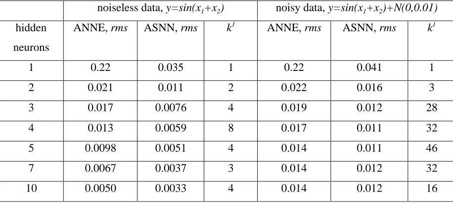
Table 1.Performance of ANNE and ASNN for Sine Function Approximation

noiseless data, y=sin(x1+x2) noisy data, y=sin(x1+x2)+N(0,0.01)

hidden

neurons

ANNE, rms ASNN, rms k1 ANNE, rms ASNN, rms k1

1 0.22 0.035 1 0.22 0.041 1

2 0.021 0.011 2 0.022 0.016 3

3 0.017 0.0076 4 0.019 0.012 28

4 0.013 0.0059 8 0.017 0.011 32

5 0.0098 0.0051 4 0.014 0.011 46

7 0.0067 0.0037 3 0.014 0.012 32

10 0.0050 0.0033 4 0.014 0.012 16

1

Number of nearest neighbors in (5). The performance of the methods is estimated using a test set

0 0.2 0.4 0.6 0.8 1

0 π/4 π/2 3π/4 π

D

0 π/4 π/2 3π/4 π

A

0 π/4 π/2 3π/4 π

B

0 π/4 π/2 3π/4 π

C

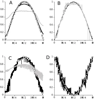
Figure 1. Sine function y=sin(x=x1+x2) approximation. For all examples the approximation

results are shown for 1000 test cases generated in Example 2 and using 100 networks in

the ensemble.

A) Sine approximation by ANNE of networks with one (gray) and two hidden neurons (black)

trained using 100 cases (circles).

B) ASNN results for the same example.

C) Sine approximation by ANNE (gray) trained with 10 cases (circles). ASNN results (black) are

shown using the same ensemble but after increasing the ASNN memory to 100 cases.

D) The ASNN results using ANNE from B) but after changing the ASNN memory to 100 cases