Volume 2010, Article ID 408109,14pages doi:10.1155/2010/408109
Research Article
Time-Frequency and Time-Scale-Based Fragile Watermarking
Methods for Image Authentication
Braham Barkat
1and Farook Sattar (EURASIP Member)
21Department of Electrical Engineering, The Petroleum Institute, P.O. Box 2533, Abu Dhabi, UAE
2Faculty of Computer Science and Information Technology, University of Malaya, 50603 Kuala Lumpur, Malaysia
Correspondence should be addressed to Farook Sattar,farook [email protected]
Received 14 February 2010; Revised 29 June 2010; Accepted 30 July 2010
Academic Editor: Bijan Mobasseri
Copyright © 2010 B. Barkat and F. Sattar. This is an open access article distributed under the Creative Commons Attribution License, which permits unrestricted use, distribution, and reproduction in any medium, provided the original work is properly cited.
1. Introduction
Watermarking techniques are developed for the protec-tion of intellectual property rights. They can be used in various areas, including broadcast monitoring, proof of ownership, transaction tracking, content authentication, and copy control [1]. In the last two decades a number of watermarking techniques have been developed [2–10]. The requirement(s) that a particular watermarking scheme needs to fulfill depend(s) on the application purpose(s). In this paper, we focus on the authentication of images. In image authentication, there are basically two main objectives: (i) the verification of the image ownership and (ii) the detection of any forgery of the original data. Specifically, in the authentication, we check whether the embedded information (i.e., the invisible watermark) has been altered or not in the receiver side.
Fragile watermarking is a powerful image content aut-hentication tool [1,7,8,11]. It is used to detect any possible change that may have occurred in the original image. A fragile watermark is readily destroyed if the watermarked image has been slightly modified. As an early work on image authentication, Friedman proposed a trusted digital camera, which embeds a digital signature for each captured image [12]. In [13], Yeung and Mintzer proposed an authentication watermark that uses a pseudorandom sequence and a mod-ified error diffusion method to protect the integrity of the images. Wong and Memon proposed a secret and a public key image watermarking scheme for authentication of grayscale images [14]. A secure watermark based on chaotic sequence
was used for JPEG image authentication in [3]. A statistical multiscale fragile watermarking approach based on a Gaus-sian mixture model was proposed in [6]. Many more fragile watermarking techniques can be found in the literature.
Most of the existing image watermarking methods are based on either spatial domain techniques or frequency domain techniques. Only few methods are based on a joint spatial-frequency domain techniques [15,16] or a joint time-frequency domain techniques [9,17]. The approach in [15] uses the projections of the 2D Radon-Wigner distribution in order to achieve the watermark detection. This watermarking technique requires the knowledge of the Radon-Wigner distribution of the original image in the detection process. In [16], the watermark detection is based on the correlation between the 2D STFT of the watermarked image and that of the watermark image for each image pixel. In [9, 17], the Wigner distribution of the image is added to the time-frequency watermark. In this technique the detector requires access to the Wigner distribution of the original image.
samples. For simplicity, and without loss of generality, we consider in the sequel a square image of sizeN×Nand the nonstationary signal of lengthNsamples only. Thelocations
of the N image pixels used to embed the N watermark samples can be chosen arbitrarily. In what follows, we choose to embed the watermark in the N diagonal pixels of the image. Alternative pixel locations can also be considered. Moreover, a pseudonoise (PN) sequence can be used as a secret key to modulate the watermark signal, making the time-frequency signature harder to perceive or to modify. In the extraction process, not all pixels of the original image are needed to recover the watermark but only thoseNpixels where the watermark has been embedded. Here, these N original pixels are inserted in the watermarked image itself. At the receiver, it is assumed that the legal user knows the locations of the watermark samples as well as the locations of the corresponding original pixels and the secret key (if used). If, for any reason, the N original pixels are not inserted in the watermarked image, they still need to be known by the legal user for the detection purpose. Once the watermark is extracted, its time-frequency representation is used to certify the original ownership of the image and verify whether it has been modified or not. If the watermarked image has been attacked or modified, the time-frequency signature of the extracted watermark would also be modified significantly, as it will be shown in coming sections.
The second proposed fragile watermarking method, based on wavelet analysis, uses complex chirp signals as watermarks. The advantages of using complex chirp signals as watermarks are manyfold, among these one can cite (i) the wide frequency range of such signals making the watermarking capacity very high and (ii) the easiness in adjusting the FM/AM parameters to generate different watermarks. In this technique, the wavelet transformation decomposes the host image hierarchically into a series of successively lower resolution reference images and their associated detail images. The low resolution image and the detail images including the horizontal, vertical, and diagonal details contain the information to reconstruct the reference image of the next higher resolution level. The detection does not require the original image, instead it uses the special feature of the extracted complex chirp watermark signal for content authentication.
Before concluding this section, we should observe that due to its inherent hierarchical structure, the wavelet-based watermarking method provides a higher level of security, and a more precise localization of any tampering (that may occur) in the watermarked image. On the other hand, the advantage of the time-frequency-based watermarking method, compared to the proposed time-scale one, lies in its simplicity and its possibility to use a larger class of nonstationary signals as watermarks.
The paper is organized as follows. In Sections2and3, we give a brief review of time-frequency analysis, introduce the time-frequency based watermarking method, and discuss its performance through some selected examples. InSection 4, we present a brief review of the discrete wavelet transform and introduce the wavelet based watermarking method. In
Section 5, we discuss the performance of the second method
through two applications: the content integrity verification with tamper localization capability and the quality assess-ment of the watermarked image. Section 6 concludes the paper.
2. Method I: Proposed Fragile Watermarking
Based on Time-Frequency Analysis
2.1. Brief Review of Time-Frequency Analysis. A given signal can be represented in many ways; however, the most impor-tant ones are time and frequency domain representations. These two representations and their related classical methods such as autocorrelation and/or power spectrum proved to be powerful in the analysis ofstationary signals. However, when the signal is nonstationary these methods fail to fully characterize it. The use of the joint time-frequency representation gives us a better understanding in the analysis of nonstationary signals. The ability of the time-frequency distribution to display the spectral contents of a given nonstationary signal makes it a very powerful tool in the analysis of such signals [18]. As an illustration, let us consider the analysis of a nonstationary signal consisting of a quadratic frequency modulated (FM) signal given by
s(t)=ΠT
t−T
2
cos2πa0t+a1t2+a2t3
, (1)
whereΠT(t) is 1 for|t| ≤ T/2 and zero elsewhere. a0,a1, anda2 are real coefficients. The signal spectrum, displayed in the bottom plot ofFigure 1, gives no indication on how the frequency of the signal is changing with time. The time domain representation, displayed in the left plot ofFigure 1, is also limited and does not provide full information about the signal. However, a time-frequency representation, displayed in the center plot of the same figure, clearly reveals the quadratic relation between the frequency and time.
Note that, theoretically, we have an infinite number of possibilities to generate a quadratic FM. This could be accomplished by just choosing different combinations of values for a0,a1, and a2. In the sequel, we will select a particular quadratic FM signal, with arbitrary start and stop times, as a watermark for our application. We emphasize here that other nonstationary signals are also feasible to choose and select.
2.2. Watermark Embedding and Extraction. As stated earlier, we can select one nonstationary signal, out of an infinite number, as our watermark. It is the particular features of this signal in the time-frequency domain that would be used to identify the watermark and, consequently, its ownership. In discrete-time domain, the selected watermark signal can be written as
s(n)=cos2πa0n+a1n2+a2n3
, n=0, 1,. . .,Nw−1. (2)
0.05 0.1 0.15 0.2 0.25 0.3 0.35 0.4 0.45 0.5 50
100 150 200 250
Frequency (Hz) Fs=1 Hz N=256
Time-res=1
T
ime
(s)
Figure1: Time-frequency representation of a quadratic FM signal: the signal’s time domain representation appears on the left, and its spectrum on the bottom.
50
100
150
200
250
50 100 150 200
250
Figure2: The original unwatermarked image used in the analysis.
the image to be watermarked. In Figure 2, we display the original unwatermarked baboonimage used in our analysis. Any arbitrary N pixels (out of the total N2 pixels) of the image are potential candidates to hide the watermark. In this presentation, we have chosen the main diagonal, from top left to bottom right, pixels as the points of interest. That is, each sample of the quadratic FM watermark signal is added to a diagonal image pixel. Note that if we choose to use the secret key, the watermark signal is first multiplied by the PN sequence and, then, added to the original diagonal pixels. Also note that in some cases, the watermark signal may have to be scaled by a real number before it is added to the original pixels. However, in our examples, we have found that a unitary scale coefficient is adequate to perform the task. The watermarked image is displayed in Figure 3. We observe that there is no apparent difference between the marked and unmarked images. In addition, the watermark is well hidden and unnoticeable.
50
100
150
200
250
50 100 150 200
250
Figure3: Watermarked image.
We stress again that (i) the number of image pixels used to embed the watermark signal samples, and (ii) their
locations in the original image can be chosen arbitrarily. Indeed, we can choose to embed all image pixels by just selecting an equal number of samples for the watermark signal. However, this number and the corresponding pixels locations used must be known to the legal user of the data.
0 0.05 0.1 0.15 0.2 0.25 0.3 0.35 0.4 0.45 0
50 100 150 200 250
Frequency [Hz]
T
ime
[samples]
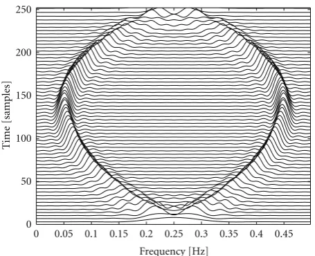
Figure4: Reduced-interference distribution of a multicomponent signal consisting of 2 quadratic FM components (with opposite instantaneous frequencies).
by (i,i+ 1), i = 1,. . .,N to contain the required original pixels. Obviously, any otherN locations(in the watermarked image) can alternatively be used to insert the original N pixels. Similarly, if the PN sequence is used, it should also be known to the legal user at the receiving end in order to extract the watermark. This sequence can also be transmitted independently or hidden in the watermark itself (using a similar procedure to the one used for the needed original pixels). Once, we have extracted the watermark samples, we use a time-frequency distribution (TFD) to analyse their content.
In the literature, we can find many TFDs. The choice of a particular one depends on the specific application at hand and the representation properties that are suitable for this application. Since we select a monocomponent quadratic FM signal as the watermark (refer to Figure 1), thus, we can clearly and unambiguously recognise our time-frequency signature by simply using a windowed Wigner-Ville distribution (WVD) of the signal. The windowed WVD is defined as [18]
Wt,f=
+∞
−∞w(τ)z
t+τ
2
·z∗
t−τ
2
e−j2π f τdτ, (3)
wherez(t) is the analytic signal associated with the water-mark signals(t) andw(τ) is the considered window. If we decide to use a more complex watermark signal such as the multicomponent signal displayed inFigure 4, the WVD would not be appropriate as it would have cross-terms which might hide the actual feature of our signature. In this case, a reduced interference TFD is more appropriate to use [19, 20]. The watermarking procedure used for multicomponent signals is similar to that used for monocomponent signals. Consequently, one can select any arbitrary pattern in the time-frequency domain as a signature without any additional computational load compared to the illustrative quadratic FM signal used in our examples.
3. Results and Performance for Method I
In this section, we evaluate the performance of the proposed fragile watermarking method. For that, we consider the time-frequency analysis of the extracted watermark when the watermarked image has been subjected to some common attacks such as cropping, scaling, translation, rotation, and JPEG compression.
For the cropping, we choose to crop only the first row of pixels of the watermarked image (leaving all the other rows untouched); for the scaling we choose the factor value 1.1; for the translation we choose to translate the whole watermarked image by only 1 column to the right; for the rotation we rotate the whole watermarked image by 1 deg anticlockwise; for the compression we choose a JPEG compression at quality level equal to 99%. Visually, the effect of these attacks on the watermarked image is unnoticeable. This is because the chosen values are very close to the values 1 (i.e., no scaling), 0 (i.e., no translation), 1 deg (i.e., slight rotation), and 100% (i.e., no compression). For space limitations, the various attacked watermarked images are not shown here (they look very similar to the unattacked watermarked image displayed
inFigure 3).
Before presenting the results that correspond to the images subjected to attacks, let us present here the TFD of the extracted watermark when there has been no attack. In
Figure 5(a), we display the TFD of the extracted watermark
when the PN has not been dealt with yet and inFigure 5(b) we display the TFD of the extracted watermark after we decode the watermark using the correct PN code. It is clear from these two figures that any attempt by an illegal user to identify the owner of the image from the TFD without knowing the correct PN code (i.e., the secret key) would not be possible.
In the following examples, we have not used the PN sequence in the watermarking process in order to focus on the effects of the attacks only (we obtained similar results when the PN is used). From each attacked image, we extract the watermark signal, as discussed in the previous section, and analyze it using a windowed WVD. The results of this operation are shown inFigure 6. These TFDs are drastically distorted in comparison with the TFD of the watermark signal extracted from the unattacked watermarked image
(seeFigure 5(b)).
Although the plots inFigure 6show the visual impact of the considered attacks on the watermark time-frequency rep-resentations, they do not quantify the amount of distortion caused to the watermark or image. To quantify the distortion, we need to evaluate the similarity, expressed in terms of the
normalized correlation coefficient,r, between the TFD of the extracted watermark and that of the original watermark. We define this normalized correlation coefficient as
r =
p
k=1w(k)·w(k) p
k=1w2(k)· p k=1w
2(k), (4)
0 0.05 0.1 0.15 0.2 0.25 0.3 0.35 0.4 0.45 0
50 100 150 200 250
Frequency [Hz]
T
ime
[samples]
(a)
0 0.05 0.1 0.15 0.2 0.25 0.3 0.35 0.4 0.45 0
50 100 150 200 250
Frequency [Hz]
T
ime
[samples]
(b)
Figure5: TFDs of the extracted watermark with no attack: (a) before removing the PN effect and (b) after removing the PN effect.
of the extracted watermark. p is the total number of time-frequency points in the respective TFDs under consideration. The value ofrbelongs to the interval [−1,1], and is equal to unity if the TFD of the extracted watermark and that of the original watermark are exactly the same.Table 1displays the values ofrthat correspond to the attacks considered earlier. These values are quite low, indicating that the proposed watermarking scheme is very sensitive to the small changes that may result from various types of attacks.
It is worth observing that any attack on the watermarked image that (i) does not affect any of the pixels where the watermark signal is embedded and, in addition, (ii) does not result in the relocation of any of these embedded pixels from its original position when it was watermarked, will not be detected at the receiver end. However, this situation can be easily avoided by increasing the watermark nonstationary signal length to watermark a larger number of the original image pixels. As stated above, the length of the watermark signal can be chosen equal up to the total number of the pixels of the unwatermarked original image.
4. Method II: Proposed Fragile Watermarking
Based on Time-Scale Analysis
In this proposed fragile multiresolution watermarking scheme a complex FM chirp signal will be embedded, using a wavelet analysis, in the original image.
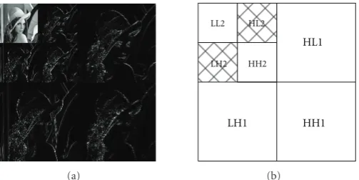
A discrete wavelet transform is used to decompose the original image into a series of successively lower resolution reference images and their associated detail images. The low-resolution image and the detail images, including the hori-zontal, vertical, and diagonal details, contain the information needed to reconstruct the reference image at the next higher resolution level.
4.1. Brief Review of the Discrete Wavelet Transform (DWT).
The two-dimensional DWT, of a dyadic decomposition type,
Table1: Similarity measure between the TFD of the original water-mark and that of the extracted waterwater-mark, when the waterwater-marked image is subjected to various attacks.
Type of Attack Correlation coefficient,r
Scaling (factor 1.1) −0.0027
Translation −0.0453
Rotation(1 degree) −0.0072
Cropping −0.0094
JPEG (QF=99%) 0.2027
considered here is given by [21]
xLLJ (n1,n2)=
i1,i2
h(i1)h(i2)xLLJ−1(2n1−i1, 2n2−i2),
xLHJ (n1,n2)=
i1,i2
h(i1)g(i2)xLLJ−1(2n1−i1, 2n2−i2),
xHLJ (n1,n2)=
i1,i2
g(i1)h(i2)xLLJ−1(2n1−i1, 2n2−i2),
xHHJ (n1,n2)=
i1,i2
g(i1)g(i2)xLLJ−1(2n1−i1, 2n2−i2),
(5)
whereh(i) represents the low-pass filter,g(i) the high-pass filter, J the DWT decomposition level, and x0LL the input image with (i1,i2)∈[0,. . ., 15].
Figure 7illustrates a two-level wavelet decomposition of
0 0.05 0.1 0.15 0.2 0.25 0.3 0.35 0.4 0.45 0
50 100 150 200 250
Frequency [Hz]
T
ime
[samples]
(a)
0 0.05 0.1 0.15 0.2 0.25 0.3 0.35 0.4 0.45 0
50 100 150 200 250
Frequency [Hz]
T
ime
[samples]
(b)
0 0.05 0.1 0.15 0.2 0.25 0.3 0.35 0.4 0.45 0
50 100 150 200 250
Frequency [Hz]
T
ime
[samples]
(c)
0 0.05 0.1 0.15 0.2 0.25 0.3 0.35 0.4 0.45 0
50 100 150 200 250
Frequency [Hz]
T
ime
[samples]
(d)
0 0.05 0.1 0.15 0.2 0.25 0.3 0.35 0.4 0.45 0
50 100 150 200
Frequency [Hz]
T
ime
[samples]
(e)
(a)
LL2 HL2
HH2 LH2
HL1
HH1 LH1
(b)
Figure7: A two-level wavelet decomposition of the Lena image.
Original image I DWT C
Key
Embedding
algorithm IDWT
Watermarked imageX
FM signals PCM Watermarkbitsw
110010100010. . .
C
Figure8: The block diagram of the proposed wavelet-based watermarking technique.
4.2. Proposed Multiresolution Watermark Embedding Scheme.
Figure 8displays a block diagram of the proposed
multires-olution watermarking technique. The various steps of this technique are described below.
Step 1(discrete wavelet transform of the original image). A levell(in the following analysis we usel=3) DWT of the original imageIis performed using Harr bases. The obtained wavelet coefficients are denoted asC.
Step 2(generation of the watermark bits). Every value of the real part,ai, and every value of the imaginary part,bi, of the unitary amplitude watermark complex sample,si=ai+jbi, is quantized into an integer value from 0 to 127. Each of the quantization values is digitally coded using a 7-bit digital code.
Specifically, a given real part valueai, is digitally coded into a 7-bit code labeledain, where nrepresents one of the 7 digit positions in this 7-bit code (i.e.,ntakes of the values from 1 to 7). In a similar way, a given imaginary part value bi, is digitally coded into a 7-bit code labeledbin.
Step 3 (generation of the key). A random sequence is
generated and used to randomly select the various image pixels to be used in the watermarking process.
Step 4(procedure to embed the watermark). The embedding of a particular watermark bit 0 or 1 is based on the QIM quantization technique [23]. To elaborate more, let us denote the lth level wavelet coefficient of the original image as Ck,l(p,q), where the subscriptk = hstands for horizontal
detail coefficient,k=vstands for vertical detail coefficient,
l=1,. . ., 3, and (p,q) are the indices of the spatial location
under consideration. Note that for an image of size (256×
256), (p,q) ∈ [1,. . ., 128] for l = 1, whereas (p,q) ∈
[1,. . ., 64] for l = 2 and (p,q) ∈ [1,. . ., 32] for l = 3,
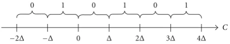
respectively. In order to embed a watermark sample consists of a real part and an imaginary part with 7 bits, we consider an image block of size (16×8). An illustrative example is shown in Figure 9 to embed 7 bits of both the real and imaginary parts of a watermark sample at different levels. As we see inFigure 9, the first bit or the most significant bit (MSB) is embedded in the third level (l =3), second and third bits are embedded in the second level (l = 2) and the last four bits are used to embed at level one (l = 1). The HL and LH bands are selected for watermark embedding as illustrated inFigure 9and the corresponding wavelet coefficient is mapped into a value 0 or 1, according to the quantization function Q(·) given by [23] (refer to
Figure 10for a graphical illustration)
Q(C)=
⎧ ⎨ ⎩
0 ifzΔ≤C <(z+ 1)Δforz=0,±2,. . .,
1 ifzΔ≤C <(z+ 1)Δforz= ±1,±3,. . ., (6)
Level 1
Level 2
Level 3 A cluster of
coefficients from sub-bands containing horizontal details
A cluster of coefficients from
sub-bands containing vertical details
1×1
2×2
4×4
1st
watermark bit 2ndand 3rd watermark bits
4th–7th watermark bits (p,q)
(p+ 1,q)
The embedding locations forain
The embedding locations forbin
Figure9: A pair of clusters of wavelet coefficients for embedding a pair ofith watermark samples ofainandbin,n=1, 2,. . ., 7.
0 1
−2Δ −Δ Δ 2Δ 3Δ 4Δ
1 0 1
0 0
C
Figure10: The quantization procedure of a given wavelet coeffi -cient.
no change in this wavelet coefficientC(i) is necessary; that is, the watermarked wavelet coefficientC(i) is
C(i)=C(i). (7)
IfQ(C(i))=/ w(i), the wavelet coefficientC(i) is then shifted to its nearest neighboring quantization step as given by
C(i)=Δround
C(i)
Δ
+Δ
2, (8)
where the operation “round(·)” is to round the element to the nearest integer towards positive infinity. The water-marked wavelet coefficients are then dispersed using the generated key.
Step 5 (inverse wavelet transform). The final watermarked image Xis obtained by an inverse DWT of C, using Harr bases.
4.3. An Illustrative Example. To illustrate the validity of the above proposed method, we consider to watermark a Lena image. In this example, we use a level 3 DWT. The
quantization steps selected here are the same as those used in [23]. Specifically, we setΔ=16, 8, 4 forl=3, 2, 1, respectively. The result of the operation is displayed inFigure 11.
We recall here that the quality of the watermarked image depends on the choice of the quantization step Δ. The smaller the value of Δ, the higher the PSNR of the watermarked image [24]. For an original image,I(n1,n2) and its watermarked image,W(n1,n2), with 255 gray levels, the PSNR is defined as [24]
PSNR=10 log10
n1 n2(255)
2
n1 n2(I(n1,n2)−W(n1,n2))
2
. (9)
In our Lena example, the PSNR of the watermarked image displayed in Figure 11(b) is found to be equal to 45.97 dB.
4.4. Watermark Extraction and Performance Against Attacks
4.4.1. Watermark Extraction Procedure. This section presents the procedure to extract the watermark at the receiver end. We observe that the extraction procedure is blind. That is, neither the original unwatermarked image nor the original watermark are required in the extraction and verification stages. However, the legal user needs to know the key used in the random permutation for the embedding locations, the wavelet type, the values of the quantization parameterΔ, and the quantization functionQ(·) [23].
Figure 12 displays a block diagram of the watermark
(a) (b)
Figure11: Watermark embedding example: (a) unwatermarked Lena image and (b) watermarked Lena image (PSNR=45.97 dB).
Watermarked
imageX DWT
Key
Extraction algorithm
110010100010. . .
Extracted watermark sampless Extracted watermark
bitsw
Conversion
In the absence of the original watermarks Authentication
and assessment
Authentication and assessment
Decision Decision
C
Figure12: A block diagram illustrating the watermark extraction and verification procedure.
Step 1 (DWT of the received image). The received image
denoted as X, could be the watermarked imageX or the watermarked image altered by attacks. A levell(the same as that used in the embedding process) DWT of the received image X is performed using Harr bases. The resulting wavelet coefficients are denoted asC.
Step 2 (Extraction of the watermark bits). Based on the watermark embedding locations provided by the key, each of the wavelet coefficients, obtained in Step 1, is quantized into the symbol “0” or “1”, using the same quantization function employed during the embedding process, namely, (6). The extracted watermark bits{w(i) ∈ (ain,bin)} are, then, extracted from odd and even quantization of the above found wavelet coefficients [23], according to
w(i)=QC(i), (10)
whereain andbin are the extracted real part and imaginary part of the complex watermark signal sample at time instant
n.
The extracted watermark bits are used to reconstruct the original watermark sample,si (=ai+ jbi), in the following
way:
wa(i)=
7
n=1
ain·27−n, wb(i)=
7
n=1
bin·27−n,
ai=
wa(i)
63.5 −1, b
i =
wb(i)
63.5 −1.
(11)
Without resorting to the original watermark, the image content authentication can be performed by simply evaluat-ing the magnitude of the extracted chirp watermark signal. This magnitude should be constant and equal to unity since our original watermark is an FM complex chirp signal with magnitude that is equal to one.
4.4.2. Performance Against Attacks. Here, we investigate the sensitivity of the proposed watermarking scheme for the following attack scenarios:
(i) JPEG compression of quality factors 90%, 80%, 70%, 60%, 50%, and 40%;
(ii) histogram equalization (uniform distortion); (iii) sharpening (low-pass filtering)—processed by Adobe
Table2: Bit error rate (BER) values of the extracted watermarks obtained for the JPEG compression attacks for various values of the quality factor (QF), and at each DWT levell.
Example: Lena image
QF l=3 l=2 l=1
90% 0 0.0728 0.4587
80% 0.0068 0.1880 0.4802
70% 0.0313 0.2847 0.4832
60% 0.0781 0.3413 0.5034
50% 0.1357 0.4214 0.4995
40% 0.2168 0.4634 0.4978
Table3: Bit error rate (BER) values of the extracted watermarks obtained for other types of attacks, and at each DWT levell.
Attacks Example: Lena image
l=3 l=2 l=1
No attacks 0 0 0
Histogram equalization 0 0.0728 0.4587 Sharpening 0.0068 0.1880 0.4802 Blurring 0.0313 0.2847 0.4832 Gaussian noise 0.0781 0.3413 0.5034 Salt-and-pepper noise 0.1357 0.4214 0.4995
(iv) blurring (high-pass filtering)—processed by Adobe Photoshop 7.0;
(v) additive Gaussian noise (variance=0.01);
(vi) Salt-and-pepper noise (This type of noise is typically seen on images with impulse noise model and represents itself as randomly occurring white and black pixels with value set to 255 or 0, resp.).
Specifically, we evaluate the performance of the pro-posed watermarking technique by considering the extraction of the watermark from the watermarked Lena image in
Figure 11(b), when subjected to each of the above attacks.
The performance is measured in terms of the bit-error-rate (BER) of the extracted watermark bits, and is defined as
BER= Ne
Nw
, (12)
whereNe is the number of bits in error andNw is the total number of watermark bits used in the watermarking process. In our Lena example, we used a level 3 DWT; conse-quently, the BER of the extracted watermark of all three wavelet decomposition levels are evaluated. In Table 2 we provide the obtained BER values for the different JPEG compressions attacks, and in Table 3 we provide the BER values that correspond to the other types of attacks.
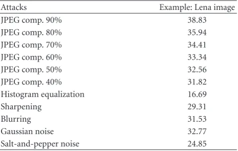
In addition, we have evaluated the PSNR of the distorted watermarked image for each of the attacks stated above. The results are summarized inTable 4.
We note that the watermark embedded in a higher decomposition level (low frequency band) has better resis-tance against distortions. Also, note that the embedded
Table 4: Peak signal-to-noise ratio (PSNR) values (in dB) of the distorted watermarked Lena image when subjected to various attacks.
Attacks Example: Lena image
JPEG comp. 90% 38.83
JPEG comp. 80% 35.94
JPEG comp. 70% 34.41
JPEG comp. 60% 33.34
JPEG comp. 50% 32.56
JPEG comp. 40% 31.82
Histogram equalization 16.69
Sharpening 29.31
Blurring 31.53
Gaussian noise 32.77
Salt-and-pepper noise 24.85
watermark can be fully recovered without any bit error when there is no attack.
5. Performance Study for Method II
In this section we demonstrate the performance of the wavelet-based watermarking method through two appli-cations. In the first application we study the content integrity verification with localization capability. In the second application, we study the quality assessment of the watermarked content by investigating the extracted complex chirp watermark in the absence of the original watermark.
5.1. Content Integrity Verification without Resorting to the
Original Watermark. Here we present how to check the
integrity of the watermarked image content, and how to localize any tamper in the image, without knowing the orig-inal watermark. Specifically, our aim is to detect and locate any malicious change, such as feature adding, cropping, and replacement that may have occurred in the watermarked image. The detection is performed by simply extracting the watermark complex chirp signal and, then, evaluating its magnitude. Recall that this magnitude should be constant and equal to unity if the watermarked image has not been subjected to any attack.
As an illustration, consider a Lena image of 256×256 pixels. The Lena image is virtually partitioned into blocks of size 16×8 pixels each. The resulting 512 blocks are labeled from 1 to 512 in a columnwise order, as shown inFigure 13. The watermark complex signal length is chosen equal to 512 samples. Each of these is embedded (using our proposed scheme) in one of the 512 image blocks; whereby, the upper 8×8 pixels of the block are used to embed the sample real part and the lower 8 × 8 pixels of the block are used to embed the sample imaginary part. Note that, for simplicity and illustrative purpose, we assume here that no random permutation key is used.
1
1 1
256 pixels
Each box denotes a block of 16×8 pixels 2
16 17
18
32
50 49
48 34
33 497
64
498
512 . . . . . . . . . . . . . . . . . .
. . .
. . .
. . .
256
pix
els
Figure13: Virtual partitioning of a Lena image of size 256×256 pixels into blocks of size 16×8 pixels each, and indexed from 1 to 512 in a columnwise order.
0 50 100 150 200 250 300 350 400 450 500 0.95
1 1.05 1.1 1.15 1.2 1.25 1.3
Block index
M
ag
n
itude
o
f
the
ex
tr
act
ed
chir
p
sig
nal
Figure 14: Magnitudes of watermark samples obtained for each of the 512 blocks, when no alteration occurs in the received watermarked image.
magnitude almost equal to one.Figure 14displays the result of the detection operation for our example. As expected, the magnitude of each sample is approximately equal to unity.
Now we assume that the Lena image has been subjected to an attack. First, we consider that the attack has occurred in one single block. Then, we generalize the assumption to multiple blocks.
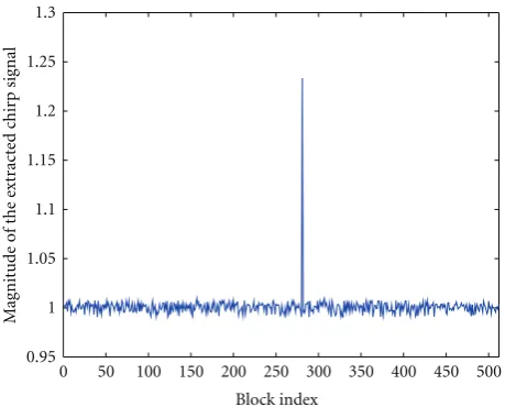
5.1.1. Tamper in a Single Authentication Block. Here, we assume that the watermarked Lena image is altered in only one pixel. Specifically, we assume that the value of the pixel located at (135, 138) has been changed from 196 to 0, as shown inFigure 15.
The pixel under consideration belongs to the 16 ×
8 authentication block with index 281, as illustrated in
Figure 16.
Figure15: A tampered watermarked Lena image. The pixel value located at (135, 138) is set to 0 (indicated by a black dot in the left eye region).
1
1 256
(135, 138)
144
137
129
144
136
16×8 authentication block with index
281
256
Figure16: Position of the altered pixel in the watermarked image.
The detector response in this case presents a magnitude value different from unity at the block index 281, as shown
in Figure 17. This is an indication that an alteration has
occurred at this specific block location of the watermarked image.
5.1.2. Tampers in Multiple Authentication Blocks. Here, we assume that the watermarked Lena image is altered in more than one authentication blocks.
Assume that the mouth region of the watermarked Lena image has been deliberately replaced by a different mouth image. The result of this operation is shown inFigure 18(a).
Figure 18(b) displays the region (i.e., the mouth region)
where the alteration occurred.
As we can see, it is difficult to pinpoint, at the naked eye, to the exact block locations where the alteration occurred
in Figure 18(a). However, our detector as can be seen
in Figure 19(a), is able to indicate the indexes of all ten
0 50 100 150 200 250 300 350 400 450 500 0.95
1 1.05 1.1 1.15 1.2 1.25 1.3
Block index
M
ag
n
itude
o
f
the
ex
tr
act
ed
chir
p
sig
nal
Figure 17: Magnitudes of watermark samples obtained for each of the 512 blocks, when an alteration occurs in one block of the received watermarked image.
Table5: Quality assessment using the mean square error (MSE) and the signal-to-noise ratio (SNR) of the extracted watermark signal, when the watermarked Lena image is JPEG compressed, using various compression quality factor values.
JPEG Comp. Actual PSNR Quality Assessment
(QF) (dB) MSE SNR (dB)
100% 45.97 2.0025×10⁻⁵ 46.98
99% 45.35 5.1460×10⁻⁴ 32.89
98% 44.41 0.0014 28.69
95% 41.53 0.0101 19.95
90% 38.83 0.0267 15.74
80% 35.94 0.0641 11.93
70% 34.41 0.0956 10.19
60% 33.34 0.1061 9.74
50% 32.56 0.1227 9.11
given by 267, 268, 283, 284, 299, 300, 315, 316, 331, and 332, exactly match the indexes of the blocks that we deliberately modified earlier. The positions and indexes of the altered blocks are shown inFigure 19(b).
5.2. Quality Assessment of the Proposed Method II. In this section, we discuss the quality assessment of the received watermarked image, when subjected to various attacks. Ideally, the magnitude of each extracted watermark sample is equal to unity; however, in practice, the actual value is different from one due to the possible manipulations of the watermarked image content. This point is well illustrated in
Figure 20.
We evaluate the level of distortion of the attacked water-marked image by evaluating the mean square error (MSE) between the actual magnitude of the extracted watermark
Table6: Quality assessment using the mean square error (MSE) and the signal-to-noise ratio (SNR) of the extracted watermark signal, when the watermarked Lena image is altered by various attacks.
Attacks Quality Assessment
MSE SNR (dB)
Histogram equalization 0.1282 8.92
Sharpening 0.1038 9.84
Blurring 0.1062 9.74
Gaussian noise 0.1202 9.20
Salt-and-pepper noise 0.0926 10.34
signal and its original value (i.e., unity). Mathematically, the MSE is computed as
MSE= 1
Nw
Nw
i=1
mag(i)−12, (13)
where mag(i) denotes the magnitude of the ith extracted watermark sample, and Nw is the number of watermark samples embedded in the image.
Equivalently we can evaluate, in (dB), the quality mea-sure of the distortion, in terms of the signal-to-noise ratio (SNR) as follows:
SNR=10 log10
1 MSE
. (14)
Note that the further is the extracted watermark signal from the original watermark one, the larger is the value of the MSE, and, consequently, the smaller is the value of the SNR.
Table 5 summarizes the results, when the watermarked
Lena image (refer toFigure 11) is subjected to JPEG com-pression for various quality factor values. As expected, we observe that the MSE increases (i.e., SNR decreases) with decreasing quality factor values.
In the same table, we also show the PSNR values obtained in this case. These values confirm the degradation of the attacked image with decreasing JPEG quality factor.
We note that the MSE obtained for the JPEG compression quality factor 100% (i.e., no attack) is nonzero. This is due to the quantization noise (refer to earlier sections), and can be reduced by reducing the quantization step used in the watermarking procedure.
Table 6 summarizes the results when the image is
sub-jected to other attacks. The corresponding PSNR values (in dB) for these attacks were already given inTable 4. We note that the amount of image content degradation increases with increasing MSE values (i.e., decreasing SNR values).
6. Conclusion
(a) (b)
Figure18: (a) A tampered watermarked Lena image, and (b) the region around the mouth indicates where the alteration occurred (a).
0 50 100 150 200 250 300 350 400 450 500 0.3
0.4 0.5 0.6 0.7 0.8 0.9 1 1.1 1.2 1.3
Block index
M
ag
nitude
o
f
the
ext
rac
te
d
chir
p
sig
nal
(a)
16×8 authentication
block
Block index
267 283 299 315 331
268 284 300 316 332
Pixel location (161, 129)
(192, 129) (192, 168)
(161, 168)
Block index
(b)
Figure19: (a) The detector response after analysis ofFigure 18(a)(“◦” indicates the indexes of the blocks affected by the alteration). (b) Indexes and positions of the altered blocks in the attacked watermarked image.
Time (sample)
M
ag
nitude
o
f
ext
ra
ct
ed
co
mp
lex
chir
p
si
gn
al
Ideal curve Actual
curve
1
0
Figure20: Ideal and actual magnitudes of the extracted watermark signal.
the first method, the watermark consists of an arbitrary nonstationary signal with a particular signature in the time-frequency plane. This method can allow the use of a secret
deals with a content integrity verification without restoring to the original watermark and the second application deals with a blind quality assessment of the received watermarked image.
References
[1] I. J. Cox, M. L. Miller, and J. A. Bloom,Digital Watermarking, Morgan Kaufmann, San Mateo, Calif, USA, 2002, An Imprint of Academic Press.
[2] S.-J. Lee and S.-H. Jung, “A survey of watermarking techniques applied to multimedia,” in Proceedings of the IEEE Interna-tional Symposium on Industrial Electronics (ISIE ’01), pp. 272– 277, June 2001.
[3] H. Wang and C. Liao, “JPEG images authentication with dis-crimination of tampers on the image content or watermark,”
IETE Technical Review, vol. 27, no. 3, pp. 244–251, 2010. [4] C.-C. Wang and Y.-C. Hsu, “New watermarking algorithm
with data authentication and reduction for JPEG image,”
Journal of Electronic Imaging, vol. 17, no. 3, article no. 033009, 2008.
[5] S. Suthaharan, “Fragile image watermarking using a gradient image for improved localization and security,”Pattern Recog-nition Letters, vol. 25, no. 16, pp. 1893–1903, 2004.
[6] H. Yuan and X.-P. Zhang, “Multiscale fragile watermarking based on the Gaussian mixture model,”IEEE Transactions on Image Processing, vol. 15, no. 10, pp. 3189–3200, 2006. [7] C.-C. Wang and Y. C. Hsu, “Fragile watermarking scheme for
H.264 video authentication,”Optical Engineering, vol. 49, no. 2, 2010.
[8] P. MeenakshiDevi, M. Venkatesan, and K. Duraiswamy, “A fragile watermarking scheme for image authentication with tamper localization using integer wavelet transform,”Journal of Computer Science, vol. 5, no. 11, pp. 831–837, 2009. [9] Y. Zhang, B. G. Mobasseri, B. M. Dogahe, and M. G. Amin,
“Image-adaptive watermarking using 2D chirps,” Signal, Image and Video Processing, vol. 4, no. 1, pp. 105–121, 2010. [10] L. Le and S. Krishnan, “Time-frequency signal synthesis and
its application in multimedia watermark detection,”Eurasip Journal on Applied Signal Processing, vol. 2006, Article ID 86712, 14 pages, 2006.
[11] X. Zhang and S. Wang, “Fragile watermarking scheme using a hierarchical mechanism,”Signal Processing, vol. 89, no. 4, pp. 675–679, 2009.
[12] G. L. Friedman, “Trustworthy digital camera: restoring cred-ibility to the photographic image,” IEEE Transactions on Consumer Electronics, vol. 39, no. 4, pp. 905–910, 1993. [13] M. M. Yeung and F. Mintzer, “Invisible watermarking
tech-nique for image verification,” inProceedings of the Interna-tional Conference on Image Processing (ICIP’ 97), vol. 2, pp. 680–682, October 1997.
[14] P. W. Wong and N. Memon, “Secret and public key image watermarking schemes for image authentication and owner-ship verification,”IEEE Transactions on Image Processing, vol. 10, no. 10, pp. 1593–1601, 2001.
[15] S. Stankovi´c, I. Djurovi´c, and L. Pitas, “Watermarking in the space/spatial-frequency domain using two-dimensional Radon-Wigner distribution,” IEEE Transactions on Image Processing, vol. 10, no. 4, pp. 650–658, 2001.
[16] S. Stankovic, I. Orovic, and N. Zaric, “An application of multidimensional time-frequency analysis as a base for the unified watermarking approach,”IEEE Transactions on Image Processing, vol. 19, no. 3, pp. 736–745, 2010.
[17] B. G. Mobasseri, “Digital watermarking in joint time-frequency domain,” inProceedings of the International Confer-ence on Image Processing (ICIP ’02), pp. 481–484, September 2002.
[18] F. Hlawatsch and G. F. Boudreaux-Bartels, “Linear and quadratic time-frequency signal representations,”IEEE Signal Processing Magazine, vol. 9, no. 2, pp. 21–67, 1992.
[19] H. Choi and W. J. Williams, “Improved time-frequency representation of multicomponent signals using exponential kernels,”IEEE Transactions on Acoustics, Speech, and Signal Processing, vol. 37, no. 6, pp. 862–871, 1989.
[20] J. Jeong and W. J. Williams, “Kernel design for reduced inter-ference distributions,”IEEE Transactions on Signal Processing, vol. 40, no. 2, pp. 402–412, 1992.
[21] S. Mallat,A Wavelet Tour of Signal Processing, Academic Press, Amsterdam, The Netherlands, 1999.
[22] L. Lin, “A survey of digital watermarking technologies,” Tech. Rep., Stoney Brook University, New York, NY, USA, 2005. [23] D. Kundur and D. Hatzinakos, “Digital watermarking for
telltale tamper proofing and authentication,”Proceedings of the IEEE, vol. 87, no. 7, pp. 1167–1180, 1999.