Limiting spectral distribution of the sample covariance matrix of the windowed array data

R E S E A R C H

Open Access

Limiting spectral distribution of the sample

covariance matrix of the windowed array data

Ehsan Yazdian

, Saeed Gazor

and Mohammad Hasan Bastani

Abstract

In this article, we investigate the limiting spectral distribution of the sample covariance matrix (SCM) of

weighted/windowed complex data. We use recent advances in random matrix theory and describe the distribution of eigenvalues of the doubly correlated Wishart matrices. We obtain an approximation for the spectral distribution of the SCM obtained from windowed data. We also determine a condition on the coefficients of the window, under which the fragmentation of the support of noise eigenvalues can be avoided, in the noise-only data case. For the commonly used exponential window, we derive an explicit expression for the l.s.d of the noise-only data. In addition, we present a method to identify the support of eigenvalues in the general case of signal-plus-noise. Simulations are performed to support our theoretical claims. The results of this article can be directly employed in many applications working with windowed array data such as source enumeration and subspace tracking algorithms.

1 Introduction

The distribution of the eigenvalues of the sample covari-ance matrix (SCM) of data has important impact on the performance of signal processing algorithms. Over the last decade, the properties of complex Wishart matri-ces are used in the analysis and design of many signal processing algorithms such as in array processing. Our knowledge about the distribution of eigenvalues, eigen-vectors and determinants of complex Wishart matrices and their limiting behavior is emerging as a key tool in a number of applications, e.g., in data compression and analysis of wireless MIMO channels [1,2], array process-ing, source enumeration and identification [3-5], adaptive algorithms [6,7]. The densities of the singular values of random matrices and their asymptotic behavior (as the matrix size tends to infinity) has been employed in some applications [8-10]. The eigenvalues of the SCM are often used to describe many signal processing problems. For example in [8], they are used as sufficient statistics for array source enumeration.

LetX1,. . .,XN beN independent zero mean Gaussian

random vectors with covariance matrix of A, i.e., NM(0,A), where Ais a nonnegativeM×MHermitian

*Correspondence: [email protected]

1Department of Electrical and Computer Engineering, Isfahan University of Technology, Isfahan, Iran

Full list of author information is available at the end of the article

matrix. The SCMRNis defined asRN = _N1Ni=1XiXH_i = 1

NXXH, whereX=[X1,. . .,XN] containsNsnapshots of

the received data. In this article, we refer to this SCM as the SCM with rectangular window (SCM-R) as all data samples have equal weights, i.e., a rectangular window is used. In this caseRN has a Wishart distribution [11] and

for more than four decades, it has been known that the joint probability density function (PDF) of its eigenvalues, can be expressed in terms of hyper-geometric functions [12]. More recently, a simpler form of this joint PDF was derived in terms of the product of two determinants [13]. However, this form is applicable if the array is small and the eigenvalues of the covariance matrix of the observed data are distinct. Several articles have investigated the behavior of the eigenvalues of RN when M,N → ∞

assuming M_N → c > 0 [14,15]. This is a more realistic assumption than assuming M is finite and N is infi-nite, because in most practical applications the covariance matrixAslowly varies, hence, the effective window length could not be arbitrary long. For instance, the eigenvalue estimators that are consistent in this asymptotic regime are more robust to finite sample size than other estima-tors which are only guaranteed to converge for fixedM

andN → ∞ [9]. There are many works on the distri-bution of eigenvalues in this asymptotic regime, such as information-plus-noise [16] and spiked models where all eigenvalues are equal excluding a small number of fixed

eigenvalues (spikes) [17]. Specifically, the distribution of the largest noise eigenvalue is widely studied [18,19].

Some signal processing algorithms process a batch of data together and deal with the SCM-R. In addition, the existing results in literature about the behavior of the eigenvalues mainly consider the rectangular window. However in a number of practical signal processing algo-rithms, the SCM is estimated by applying a window as follows

RN =

1

N N

i=1

wiXiXiH, (1)

where{wi ≥ 0,i = 1,. . .,N}is a non-negative sequence.

Hereafter, we refer to RN as the SCM. The SCM-R is

obtained using a rectangular window, i.e., where wi is

non-zero and constant for i = 1,. . .,N. These weights allow to flexibly emphasize or deemphasize some of the observations. For example smaller weights for old data samples allows to improve the agility of the algorithms. For instance in cognitive radio, it is important to detect the activities of users and the idle channels as fast as pos-sible, thereby reducing the detection time and improving the agility of the system [20,21]. Among all windows, the exponential window,wi = w0pi, is commonly used. Two

reasons for this popularity are (1) this window allows to develop fast recursive algorithms which are considerably less expensive in terms of computational complexity, thereby facilitate the real-time implementation of these algorithms (e.g. see [22,23]) and (2) allows to forget the old data, thereby improving the tracking ability in non-stationary environments. For instance exponentially windowed data is used in most of the existing subspace tracking algorithms[24,25]. That is because only a rank-one update is required for each new data vector to update the underlying SCM, which leads to simple low cost subspace tracking algorithms.

In this article, we study the effects of windowing on the distribution of the eigenvalues of the SCM. In this case, the SCM in (1) has a doubly correlated Wishart distri-bution [26-30]. We must note that, there are numerous research results for the case of Wishart matrices, however, the spectral properties in the doubly correlated case has not been sufficiently studied.

Manipulating the joint PDF of the eigenvalues which is a very complex function is not practical, particularly for large matrices. An alternative approach used in the literature, is to employ the following empirical spectral distribution (e.s.d.) of a square matrixA∈CM×M

FA(x)= 1

M#{λi≤x|i=1,. . .,M}, (2)

whereλ1,λ2,. . .,λMare eigenvalues ofAand #{.}denotes

the cardinality of a set. Note that, in this definition all eigenvalues of A are assumed to be real. Although this

formulation is less explicit than the joint PDF of values, it describes the statistical behavior of the eigen-values. In many practical casesAis a random matrix and the e.s.d. FA_{(x) is a random function which converges}

almost surly to a deterministic cumulative distribution function as the dimension of the system grows. In such cases, limM→∞FA(x)is referred to as the limiting spectral

distribution (l.s.d.) ofA.

In recent years, some results have been obtained on the limiting behavior of the e.s.d. of correlated Wishart matrices. In this article, for the white noise case, we study the behavior of eigenvalues of the SCM. In particular for the exponential window, we extend the results previously demonstrated in [31] and give more details along with the proofs of the required theorems. We then consider the case of signal plus noise and present a method to deter-mine the support of eigenvalues. The main contributions in this article are

• A method is proposed to approximate the spectral distribution of the SCM using arbitrary windows with that of an equivalent Wishart Distribution. For the especial case of white noise (noise only), this approximation is the Marchenko–Pastur (M–P) distribution, which is the known distribution for the case of a rectangular window.

• In Theorem 2, we derive an accurate and explicit equation for the l.s.d. of the SCM of noise-only data for the exponential window. Many simulations are performed to show the accuracy of this l.s.d. • In Theorem 3 we present a systematic method to

compute the support of eigenvalues in the signal plus noise data case using an exponentially weighted window. In addition to the results, we follow up a different and novel approach in proving this theorem compared with the existing proof for the rectangular window case where the Stieltjes transformm(z)has the explicit inverse [15]. This approach can be easily utilized for other window types where the Stieltjes transform is expressed explicitly or implicitly as a function ofz.

such as subspace tracking, DOA estimation and source enumeration.

The remainder of this article is organized as follows: Section 2 introduces the system model and some impor-tant mathematical tools. We derive an approximation for the Stieltjes transform of l.s.d. of eigenvalues of weighted windowed array data in Section 3. Asymptotic spectrum of the eigenvalues in noise-only data case is analyzed in Section 4. The signal plus noise case is studied in Section 5. Section 6 provides simulation results. Finally, we conclude this work and suggest future works in Section 7.

2 System model for windowed SCM

We assume thatXi ∈ CM in (1) is a circularly

symmet-rical independent Gaussian random vector process with zero mean and covariance matrix of A ∈ CM×M, i.e.,

Xi ∼ NM(0,A). In this case, we can rewrite (1),

suppos-ing that SCM is estimated ussuppos-ing a window of sizeNwith positive coefficientsw1,. . .,wN,

RN =

1

N N

i=1 wiA

1

2_UiUiH_A12 = 1

NA

1

2_UWNUH_A12_,

(3)

where U =[U1,. . .,UN] is an M× N matrix contains

i.i.d. zero-mean unit-variance complex Gaussian entries andWN=diag(w1,. . .,wN). The matrixRNhas a doubly

correlated Wishart distribution. In practice, it is very com-plex to directly characterize the e.s.d. ofRN thus, we use

the Stieltjes transform of this distribution and indirectly characterize the behavior of the eigenvalues. Then, in the asymptotic regime asM,N → ∞given M_N → c>0, the inverse transform of the limit gives the l.s.d of SCM.

Definition 1.[15]Stieltjes transform m(z), z ∈ C+ ≡ {z ∈ C : Im(z) > 0}of a distribution function FR(x)is defined as

m(z)=

1

λ−zdF

R_{(λ). (4)}

The inverse Stieltjes transform formula is as follows:

FR(x)= 1 πylim→0+

x

−∞Im{m(t+iy)}dt, ∀x∈R. (5)

Hence, in order to characterize the asymptotic distribu-tion of the sample eigenvalues, we alternatively character-ize the asymptotic behavior of the corresponding Stieltjes transform, and then use the Stieltjes inversion formula in (5) to obtain l.s.d. of SCM fR(x). We use the following theorem which gives the Stieltjes transform of the corre-lated Wishart matrix [29] and is the basis for derivations in this article.

Theorem 1.For a finite length window with length of N, consider the matrix defined by RN =

1 NAN

1

2_UWNUH_AN12. Assume that all elements of

U ∈ CM×M are i.i.d. random variables with zero-mean, unit variance and finite E{|Uij|4}. In addition, suppose that AN ∈ CM×M is a Hermitian nonnegative definite matrix,WN =diag(w1,. . .,wN), FAN→D FA, FWN→D FW when M,N → ∞ with M_N → c > 0. In this case, the empirical distribution FRN_{, with probability 1, converges} weakly to a probability distribution function FR whose Stieltjes transform m(z), for z∈C+, is given by

m(z)=

1

a _1+cwew_(z)dFW_(w)−zdF

A_{(a), (6)}

where e(z)is the unique solution of the following equation inC+

e(z)=

a

a _1+cwew_(z)dFW_(w)−zdF

A_{(a) (7)}

Proof 1.See [29] for proof. Similar results are also demonstrated in [26,28] with some differences in the assumptions on correlation matrices.

We emphasize that (6) and (7) give the exact distribution in the asymptotic regime asM,N → ∞with M_N → c>

0. Since in practice, the array dimension and/or sample size are usually finite numbers, this method gives a deter-ministic approximation for the actual sample eigenvalue distribution.

To show how this method works, we now consider the simplest case (where the distribution is well known) using a rectangular window and white Gaussian noise, i.e.,W= IN×N andA= σ2IM×M. In this case, we havedFW(w)= δ(w−1)dwanddFA(x)=δ(x−σ2)dx, whereδ(x)is the Dirac delta function. Thus with straightforward manipu-lations of (6) and (7), the Stieltjes transform is found to be the solution of

z=z(m)= σ 2

1+cσ2_m−

1

m. (8)

In this case, as expected the e.s.d. of the SCM-R,FRN(x), converges to the M–P distribution [14] as follows,

fMP(x)= d dxF

MP_(x),= max(c, 1)−1

c δ(x)

+

(x−a−)(a+−x)

2π σ2_xc a−,a+(x),

(9)

wherea_±=σ2 1±√c2anda,b(x)=

1 a≤x≤b

dFA(x) = δ(x−σ2)dx, we obtainm(z) = _σ12e(z). Thus,

from (6), we obtain

m(z)= 1

σ2 w

1+cwσ2_mdFW(w)−z

. (10)

3 Effective length of a window

In this section, we define the effective length of a win-dow which allows to approximate the distribution of the eigenvalues of windowed SCM with that of a rectan-gular window with an equivalent length, assuming that the covariance matrix of dataAsatisfies the assumptions of Theorem 1. In several existing articles some intuitive equivalent length are defined simply to extend the previ-ously existing results for the rectangular case in order to analyze the behavior of the eigenvalues in the weighted window cases [22,23].

Consider a window wi > 0 of length N and denote WN= diag(w1,. . .,wN) ∈RN×N with a converging

dis-tribution, i.e., limN→∞FWN = FW. We assume that the

sample sizeNis much larger than the array dimensionM, i.e.,cis small. It is known thatm(z)is bounded forz∈C+

[15]. Thus for 0 < c 1 we have 0 < cσ2|m|sup|w| < β < 1 where β is some constant number. It is easy to show thata_{, we have} σ2_w

1+cwσ2_m−cm1 I

i=1(−cwσ2m)i ≤ |cm|I|wσ2|I+1

1−β . This yields

_σ2_wdFW_(w)

1+cwσ2_m =c

I_O+ 1

cm I

i=1

(−cσ2m)iE{wi}, (11)

whereE{.} =(.)dFW(w)and|O| ≤ |m|₁I|₋σ2_β|I+1E{wI+1}. Since 0<c1, forI=2 and definingce=cE{w

2_} E2_{w}and

we=E{w}as the effective parameters, we can rewrite (11)

as

z≈ E{w}σ 2

1+cE_E{_{w_w2_}}σ2_m−

1

m =

weσ2

1+ceweσ2m−

1

m, (12)

where using E{w3} < sup{w2}E{w} and E{w2} <

sup{w}E{w}it is easy to show that the approximation error is bounded byσ2E{w}₁2₋β2_β.

Definition 2.The expression (12) represents the M–P distribution as in (8) for a rectangular window of length

Ne= M ce =

NE 2_{w}

E{w2_}, (13)

with all coefficients equal to we. The average weight weis a scale parameter for the eigenvalues of covariance matrix of the received data. Although we have derived the effective length for the noise only data, our results reveal that this effective window length gives accurate results for the signal plus noise case.

For the white noise data, the l.s.d. of SCM can be approximated by the M–P distribution defined in (9) by substitutingcandσ2, withceandweσ2, respectively. Note

that the effective window length is always smaller than the number of samples N. This approximation can be intu-itively interpreted as a Wishart approximation where the effect of “windowing” is approximated with a rectangu-lar window with an effective number of samples of Ne

and the covariance matrix of the received data is scaled to

Ae=weA”.

Now, we compute the effective length of the triangu-lar and the exponential windows. A triangutriangu-lar window is defined bywi = 2(1− _Ni−₋11)fori = 1,. . .,N 1 and

has the average weight of _N1N_i=1wi = 1. Using (13), the

effective length of the triangular window is

Ne=

3 2

N−1 2N−1N≈

3

4N. (14)

The exponential window is very popular in signal process-ing applications due to its simple implementation and is defined bywi=w0pifori=1, 2,. . ., wherep∈(0, 1)and w0is a normalization constant. We note that the

exponen-tial window is inherently an infinite length window. Inter-estingly, in Theorem 1 the window length and the array dimension jointly tend to infinity where limM,N→∞MN = c>0. Here for a finite array dimensionM, we first approx-imate the exponential window withNcoefficients, which is only accurate ifNis large enough such that the omitted coefficients are negligible. Asymptotically asM,Njointly tend to∞, the results from this truncated window become accurate for describing the underlying distributions using the exponential window. In this case, with some calcula-tions we obtainNe = 1−p

2

(1−p)2

(1−pN−1)2

1−p2N−2 . Thus the effective

length of the exponential window (forN1) becomes

Ne≈

1+p

1−p, (15)

which is not a function of N. As expected the effective length of the window increases as the forgetting factorp

approaches one.

4 Spectral analysis of noise-only data

function allowing to derive some explicit equations for the Stieltjes transform.

LetSF denote the support of the functionfR(x)andSc_F

shows its complement. From (5), we see thatSFconsists of

points on the real axis where the imaginary part ofm(z)is positive, i.e., the support is the union of some subintervals. Thus to find the support of the distribution of eigenvalues, we must determine such intervals. In [15], it is shown that lim_y→0+mF(x+iy)exists for allx=0, and therefore we

can define

mF(x)= lim

y→0+mF(x+iy),x∈R\ {0}. (16)

The following lemma is the key to determine these inter-vals on real axis [15].

Lemma 1 ([32], Lemma 6.1).For any c.d.f. F, let SF denote its support and Sc_F be the complement of SF. For x ∈ S_Fc, m= mF(x)is the only real solution of x = z(m) which satisfies

dz(m)

dm >0, (17)

where z(m)is the inverse function of m(z). Also conversely, for any real m in the domain of z(m)if dz_dm(m) > 0 then x=z(m)is outside the support of F.

This simply means that the supportSF, is the union of

intervals on the vertical axis wherez(m)is increasing for real values of m. According to (10), for noise only data

z(m)can be written as follows

z(m)=

_σ2_w

1+cwσ2_mdF

W_(w)− 1

m. (18)

4.1 Discrete distribution function approach

Suppose the window consists of Nd distinct weights wi,i = 1,. . .,Nd, each with multiplicityn = NNd.

There-fore as (M,N → ∞and M_N → c > 0), we can evaluate (18) in terms of the weights

z(m)= 1 Nd

Nd

i=1

σ2wi

1+cwiσ2m−

1

m. (19)

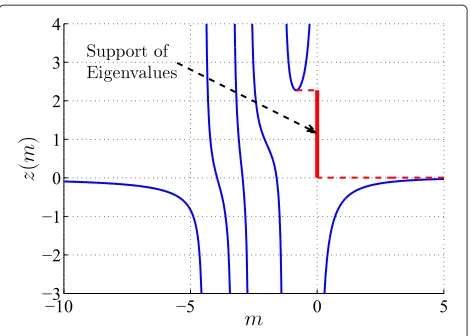
Figure 1, represent a typical case of the function on the right-hand side of (19). Lemma 1 states that the support of the distribution of eigenvalues is the complement of the set of all valuesx ∈R+for whichx = z(m)is increasing for real values ofm, i.e.,(dz_dm(m) > 0). The functionz(m)

has poles at m = 0,−_cw1

1σ2,. . .,−

1

cw_Ndσ2. In addition,

z(m)is an analytic function and we have

lim

m→0±z(m)= ∓∞, lim

m→

− 1

cwiσ2

±z(m)= ±∞. (20)

Figure 1A typical representation of the functionz(m)in (19) versusm∈Rforc<1in the case where the support of eigenvalues is a connected interval.

Forc < 1, i.e., where the length of the window is more than the array dimension, limm→±∞z(m) = 0±, thus

as Figure 1 shows, dz_dm(m) = 0 has at least two

solu-tions which we denote themmu ∈

−1 cσ2_max(wi), 0

and

m_l ∈ (0,∞). For c > 1, as Figure 2 shows typically, from limm→±∞z(m) = 0∓we conclude thatmlmust be

in

−∞,_cσ2_min−1_(wi)

. We must note that, forc > 1, the SCM hasM−Nzero eigenvalues expressed with a prob-ability mass of 1−1_cin the l.s.d. of SCM, that is not counted as a cluster in these derivations, i.e. forc >, the PDF of the distribution includes a term of 1−1_cδ(x). If the weights are widely separated, the support of eigenval-ues may become fragmented into union of a number of disjoint intervals.

In many signal processing applications the white noise subspace is separated from the signal subspace based on

the eigenvalues of the SCM. Such a fragmentation of the support of noise eigenvalues misleads the subspace based algorithms and leads to noise eigenvalues to be mistaken as signal ones.

In fact, it is desirable that the support of eigenvalues be as compact as possible. To avoid such an undesirable frag-mentation, the equation dz_dm(m) = 0 should not have real

solution form∈

−1

cσ2_min(wi),_cσ2_max−1_(wi)

, i.e.,

1

Nd Nd

i=1

1− 1 1+cwiσ2m

2

>c, (21)

∀m∈

₋

1

cσ2_min(w i)

, −1

cσ2_max(w i)

.

Under this connectivity condition, the support of eigen-values is the interval [xl = z(ml),xu = z(mu)], which

can be calculated, numerically. Our simulations show that this condition is satisfied for popular window types espe-cially forNd1 used in practice. Figure 2 shows a typical

case forc > 1 where dz_dm(m) = 0 has an even number of real-valued solutions (counting multiplicities) which we denote them by m−₁ ≤ m+₁ < · · · < m−_q ≤ m+_q (in addition to ml,mu). Each pair of these solutions

deter-mines a sub-interval for the support of eigenvalues, i.e., we have SF =[xl,xu]−{[x−1,x+1]∪ · · · ∪[x−q,x+q]}, where x−_i = z(m−_i ),x+_i = z(m+_i ). Reducingc or reducing the gap between weight values{wi}makes the support more

compact at the expense of using more temporal samples.

4.2 Continuous function approach

The goal of this approach is to find closed form expres-sions of Stieltjes integrals of the l.s.d. This approach could be used for any window shapes. However, we start with the triangular window and then consider the exponential win-dow which are more popular. Here, we model the function

fW_{(w)with a continuous distribution and evaluate (18) to}

found the Stieltjes transform.

For a triangular window wi = 2

1−_Ni−₋1₁

,i =

1,. . .,N, we haveFWN_{(w) =} 1 N

N

i=1U(w−wi) where U(w)is the unit step function. In this case it is easy to show thatFWN_{(w)converges to a uniform distribution as} Nincreases, i.e.,

lim

N→∞F

WN_(w)=_FW_(w)= ⎧ ⎨ ⎩ 1

2w, 0<w<2, 0, otherwise.

(22)

SubstitutingFW_{(w)in (18), we get}

z(m)= 1 cm

1− 1

2cσ2_mln(1+2cσ 2_m)

− 1

m, (23)

form∈(−_2c1

σ2,∞)andm=0.

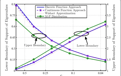
Again, we first use Lemma 1 and determine the support of eigenvalues (by plottingz(m)for realmand finding the intervals on the vertical axis wherez(m)is not increasing). Figure 3 plots the lower and upper boundaries of support of eigenvalues for a triangular window for different values ofc. It can be seen that the discrete distributionFWN_(w)

(assumingNd = 50) and the continuous approach result

in almost the same boundaries. We also observe that these boundaries are close to those obtained by the Wishart approximation assuming the effective window length in (14). In this figure using the rectangular window with same length as the triangular window, the distribution is referred to as the M–P distribution. Also we observe that the eigenvalues tend to more concentrate around their real value σ2 = 1 as the window length increases. In addition from this figure, we conclude that the support using the triangular window is looser than than that of the rectangular window for a given value ofc, because the effective length of the triangular window is less than that of a rectangular window.

For the exponential window, first we introduce the new parameter γ as the ratio of smallest to largest weights of the truncated exponential window. The coefficients of the window can be redefined as as a function of γ as

wi = w0γ i

N, i = 1,_{. . .},N. Therefore from fWN(w) =

N

i=1N1δ(w−wi), fromi= lnNγ ln

wi w0

, it is easy to show that

FWN_(w)=

⎧ ⎪ ⎪ ⎪ ⎪ ⎨ ⎪ ⎪ ⎪ ⎪ ⎩

0 w< γw0,

1− 1 N

N lnγ ln

w w0

γw0≤w≤w0γ

1

N_,

1 w0γ

1

N ≤_w,

(24)

where .is the floor function. This increasing staircase function takes values on 0,_N1,_N2,. . ., 1. To satisfy the

constraints of Theorem 1 for the exponential window, we assume that the ratio of smallest to largest weights of the window, γ = pN _{> 0, is an arbitrary small real}

con-stant. In other words, the forgetting factor of the window

p = γN1 ∈ ₍0, 1₎approaches to 1, as M,N → ∞. The

smallerγ, the better this truncated exponential model fits the exponential window with the forgetting factorp. From, limN→∞w0 = γln−γ1, we conclude that limN→∞F

WN =

FW(w)where

FW(w)= ⎧ ⎪ ⎪ ⎪ ⎪ ⎪ ⎪ ⎪ ⎨ ⎪ ⎪ ⎪ ⎪ ⎪ ⎪ ⎪ ⎩

0 w< γlnγ γ−1,

1− 1 lnγ ln

_w (γ−1)

lnγ

γlnγ γ−1 <w<

lnγ γ−1,

1 w> lnγ γ−1.

(25)

is a continuous function, independent of window sizeN

and satisfies the assumptions of Theorem 1. Thus, this theorem is applicable to the exponential window trun-cated at some large integerN.

SubstitutingFW_{(w)in (18), in the asymptotic regime of}

Theorem 1 asγ →0, such thatM_n

0 →c0,z(m)satisfies

z(m)= 1 c0m

ln 1+c0σ2m− 1

m, (26)

for allm∈−_c1

0σ2,∞

\ {0}wheren0= −_ln1(p).

One can use the same method as in the discrete dis-tribution function approach and identify the support of the distributionSF. However, the function z(m) in (26)

is simple and the following theorem gives the explicit distribution.

Theorem 2.For the exponentially weighted window, the l.s.d. of SCM, fR_{(x), is given by}

fR(x)= e c0−_σx2

πc0σ2Im

e−ω−1

−x

σ2exp

c0−_σx2

x−,x+(x),

(27)

and upper and lower boundaries of the support are

x−=σ2 ω0 −e

−c0−1+₁

exp{ω0(−exp(−c0−1))+c0+1} −1

,

(28a)

x+=σ2 ω−1(−e

−c0−1₎+₁

exp{ω₋1(−exp(−c0−1))+c0+1} −1

(28b)

respectively, where ωk(x) is the branch of Lambert W functionb[33]with k= −1and k=0.

Proof 2.According to the Lemma 1, boundaries of the support of eigenvalues are the real solutions of z(m)= 0, i.e., with some simple calculations, are the solutions of

ln 1+c0σ2m

=c0+1−

1 1+c0σ2m

. (29)

Denoting y=ln 1+c0σ2m−c0−1, we obtain

yey= −e−c0−1∈_[−e−1_{, 0),} ∀c0_{>0. (30)}

This equation has two real solutions m−and m+expressed using Lambert W function as

m−= 1 c0σ2

exp{ω0 −e−c0−1+c0+1} −1, (31)

m+= 1

c0σ2 exp{ω−1 −e

−c0−1+_c

0+1} −1

. (32)

Using(26), the boundaries z(m−)and z(m+)are obtained as in (28a) and (28b) which determine the support of eigenvalues as the interval[z(m−),z(m+)]⊂R.

To obtain the l.s.d. of SCM, we should find m(z)with pos-itive imaginary part for all z∈[z(m−),z(m+)]. In(26), we denote

v= −ln 1+c0σ2m− z

σ2+c0, (33)

and obtain

vev=− z σ2e

c0−_σz2_{. (34)}

Therefore, the solutions are

vk=ωk

− z

σ2e

c0−_σz2_, ∀k∈Z_{. (35)}

According to (16), (33), for the values of z in the inter-val of the obtained support on the real axis, due to the properties of the complex logarithm function, the imagi-nary part of v is in[−π,π], thus only the branches with k = 0 and k = −1 are acceptable solutions. It is easy to see that for z ∈[z(m−),z(m+)], the expression on the right-hand side of (34) belongs to−ec0−1_,−e−1_{. From}

(33)and properties of Lambert W function, we also deduce that Im{m}andsin(−Im{v})have the same signs, and for x ∈ −ec0−1_,−_e−1_{the functionsin(}−_Im{_ω

k(x)})is posi-tive for k = −1and is negative for k = 0. Therefore, the Stieltjes transform of the l.s.d. of SCM is obtained from(35)

and(33)as

m= 1

c0σ2 ⎛ ⎝ec0−

z

σ2−ω−1

−z

σ2e

c₀− z

σ2

−1 ⎞

⎠. (36)

Using the inverse formula in(18), the l.s.d of SCM is

fR(x)= 1 πIm

1

c0σ2

ec₀− x σ2−ω−1

− x

σ2exp

c0− x σ2

−1 .

Dropping the real terms inside the brackets and applying some simplifications, we obtain(27).

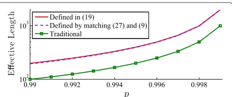
We can define a second effective window length by employing and comparing the boundaries of the support of eigenvalues in (28a) and in (9) for a rectangular window which is only in terms ofσ2andc. Equating the length of the supports in (9) (28a), i.e.,a+−a−=x+−x−, we can find a rectangular window to match the support as same as that of the exponential window and define the length of this rectangular window as another effective length for the exponential window. In some array signal processing applications, the effective length of the exponential win-dow has been considered to beNe= ₁₋1_p[22,23]. Figure 4

compares these effective lengthes in terms of the forget-ting factorpand reveals that the effective window length defined in (13) gives an accurate approximation for the exponential window. We also see a large gap between the traditional approximation for the effective length in [22] and what is obtained in this article using random matrix theory.

Remark 1.In the economic literature, other methods have been proposed to approximate the spectral density function of exponentially weighted financial covariance matrices for Portfolio Optimization[34,35]. These methods that are used in other articles (e.g., in[36,37]) are based on numerical calculations rather than developing some closed form expressions. Pafka et al.[34]supposed that the den-sity of the eigenvalues is aproximated byρ(u)= Q_πν where Q= _M(11_−p) andνis the root of

u σ2 −

uν

tan(uν) +ln(νσ

2_{)−ln(sin(uν))−} 1

Q (38)

In contrast to these methods for the exponential window, we derive an accurate explicit closed form expression which can be easily employed in many applications such as in signal processing and economy.

Figure 4Effective length of the exponential window as a function of forgetting factorp.

5 Spectral analysis of signal plus noise data In this section, we consider the case of white noise plus some signal sources, i.e., where the eigenvalues of Aare not equal. In the general case, let λq > · · · > λ1 > 0

denote the set ofqdistinct eigenvalues of the covariance matrix and the multiplicity of λ is denoted by k (we

must have M = q₌₁k). For example suppose a real

phased array communication system withq−1 indepen-dent signals impinging on it simultaneously on the same frequency band from different directions whereq < M. The smallest eigenvalueλ₁can be interpreted as the noise eigenvalue and otherq−1 larger eigenvalues are referred to as signal eigenvalues. In the asymptotic regime, when

N,Mare growing large, we assume that k

M → α > 0,

whereα, = 1,. . .,qare multiplicity ratios of

eigenval-ues. In this case the spectral distribution of the matrix

Ain Theorem 1 can be expressed as sum of Dirac delta functions, i.e.dFA(a)=q_i=1α_iδ(a−λ_i)da.

In what follows, we present an approach to determine the support of eigenvalues and also the l.s.d. of expo-nentially weighted SCM of signal plus noise data in the asymptotic regime. The first in determining the distribu-tion of the eigenvalues is to determine its support on the real positive axis.

The definition of the Stieltjes transform in (4) implies that for any distributionFand realxoutside the support of

F,m(x)is well defined and its derivative,m(x)= ₍dF_y−(_xy₎)2,

is obviously real and positive. Thus, m(z) is increasing on intervals on real line outside the support of its dis-tribution functionF[15]. Therefore, the inverse function theorem proves that its inverse exists on these intervals and shall also be increasing. For the one sided correlated Wishart matrices, where the inverse ofm(z)has an explicit expression, Lemma 1 shows that the converse of the above statements are also true [15], i.e. for any real m in the domain ofz(m), if dz_dm(m) > 0 thenx = z(m)is outside the support of the distribution. Therefore, the support of eigenvalues is a Borel subset ofR+for whichz(m)is increasing which can be determined by simply plotting the inverse functionz(m)for realm. Paul and Silverstein ([29], page 2) suggested the same method for doubly cor-related Wishart matrices if there exists an explicit inverse

z= z(m)for the limiting Stieltjes transformm(z). Unfor-tunately, for non-rectangular windows, the inverse ofm(z)

some other window types, to determine the support of eigenvalues.

From (6) and (7) we obtain

1+zm=

we

1+cwedF

W_{(w). (39)}

Substituting (25) in (39), we get

1+zm= 1 c0

ln

1−γ +c0e

1−γ +γc0e

. (40)

SubstitutingdFA_{(a)in (7) changes the integral to a}

sum-mation and we obtaine(z)as

e(z)= q

i=1

α_iλ_i

λi c0e(z)ln

1−γ+c0e(z)

1−γ+γc0e(z)

−z

. (41)

According to Theorem 1, for anyz∈C+, there is a unique solutione = e(z)for (41) inC+. In this case the Stieltjes transformm(z)is calculated from (40) as

m(z)= 1 z

1

c0ln

1−γ +c0e(z)

1−γ +γc0e(z)

−1

(42)

This expression gives the implicit relation betweenmand

z, which cannot be sorted to expressmas an explicit func-tion ofzor conversely,zas a function ofm. Defining the auxiliary variable/functionu=c0(1+zm(z))which

pro-vides a bijective relation betweeneandmfor allz=0, we have

u=ln

1−γ +c0e(z)

1−γ +γc0e(z)

. (43)

This equation reveals that the imaginary parts ofuande

have the same signs. In addition sinceγ <1,c0is real and

using the properties of the complex logarithm function in (43), we deduce thatualways lies in a strip of the positive complex plane where its imaginary part is less thanπ, i.e., the domain ofuis defined asDu = {u|0<Im{u}< π}.

Equation (43) also provides a bijective relation betweene

andu, therefore according to Theorem 1 for anyz∈ C+, there is a uniqueu∈Du, satisfying

u=c0 q

i=1

αi λi

z euu₋₁₁₋1_γ (1−γeu)−1

+c0. (44)

Defining the second auxiliary variable/function as

h= u

(1−eu_)z

1−γeu

1−γ , ∀z=0. (45)

and defineDhas its range for allz ∈ C+. Resorting (44),

we have

u= −c0 q

i=1 α_i λih+1+

c0. (46)

Proposition 1.The auxiliary variable h, as a function of u and z, has some interesting properties as:

(1) h always lies in the subsetDh⊂C+for allz∈C+. (2) forh∈Dh, z can be explicitly expressed as a function of h

z(h)= c0 h

q i=1

αi

λih+1−1

ec0

q i=1

α_iλ_ih λih+1 −₁

1−γec0

q i=1

α_iλ_ih λih+1

1−γ .

(47)

(1) For anyz∈C+, a unique h satisfying (47) exists in

h∈C|Im{h} q

i=1

c0αiλi |λih+1|2 ∈

(0,π ) !

. (48)

Proof 3.The first property can is simply implied from

(46)as the imaginary part of h and u have the same sign. Using(45)and(46), we can easily find(47). The third prop-erty is proved as follows. The constraint in(48)is obtained from Im{u} ∈(0,π )and(46). According to Theorem 1, for any z∈C+, there is a unique u∈Du, satisfying(44). The unique pair (z,u) gives an h inC+ according to (45). In order to prove the uniqueness of h, suppose that h1and h2 inC+satisfy(47)and(48). Thus,(46)yields u1,u2 ∈ Du satisfying(44). In addition, we must have u1=u2since for any z∈C+, there exists a unique u1∈Du. Thus for z and u1=u2,(45)yields that h1=h2.

Althoughz(h) in (47) is defined only forh ∈ Dh, it is

an analytic function for allh ∈ C\

0,−_λ1

1,. . .,

−1

λq

. In

addition note thatz(h)= −_h1at the roots ofq_i=1 αi

λih+1−

1=0.

Also using (46) and (47) we expressmas a function ofh

as follows

mh(h)=

1−γ c0

q i=1

αi λih+1

q i=1

αi λih+1−1

1−e−c0qi=1

α_i λ_ih+1+c0

h

1−γe−c0 q

i=1

α_i λ_ih+1+c0

,

(49)

forh∈Dh. Similar toz(h), the complex functionmh(h)is

an analytic function for allh∈Cexcept at the set of real values0,−_λ1

1,. . .,

−1

λq

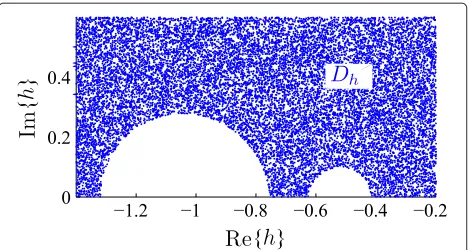
and the points wherez(h)=0. The inverse Stieltjes transform in (5) reveals that the l.s.d. depends on the behavior ofm(z)in the vicinity of the real axis, i.e. forz→x0∈R. Proposition 1 shows that the z(h)in (47) is injective overh∈ Dh ⊂ C+and allows us

to treath(z)as its inverse forz ∈ C+. To determine the range ofh(z)denoted byDhwe can evaluatez(h)for allh

Figure 5The range of the functionh(z)forz∈C+, for the case wherec0=0.2and the covariance matrix has 2 distinct eigenvalues 2 and 1 with the multiplicity ratiosα1=1₃andα2=2₃.

a covariance matrix with two distinct eigenvalues 2 and 1 with the multiplicity ratiosα1= 1₃andα2= 2₃. The white

regions in Figure 5 shows the values ofhfor whichz(h)has negative imaginary part, and the blue parts are the values where Im{z(h)} > 0. We observe that some parts of the positive complex plane are not in the domain ofz(h)as we restrict the range toz(h)∈C+.

5.1 Support of eigenvalues

Theorem 3. For the exponentially weighted window defined in Theorem 2, under the assumptions of Theorem 1, the complement of support of eigenvalues, is the set of val-ues of x = z(h)on the vertical axis where dz_dh(h) > 0for some h∈R, where z(h)is defined in (47).

Proof 4. Let SFdenotes the support of the function fR(x) and Sc_F shows its complement. To prove Theorem 3, first we show that for any x ∈ S_Fc, there exist a h ∈ Rwhere

dz(h)

dh >0. Then, we prove the converse, i.e. if dz(h)

dh >0for some h ∈ R, then x = z(h)is a real number outside the support of eigenvalues.

From(5), we see that SFconsists of points on the real axis where Im{m(x+iy)}tends to a positive number when y→

0+. Thus to find SF, we must determine such subintervals on the real axis, or equivalently we can determine S_Fc by finding the intervals on the real axis wherelimy→0+{m(x+ iy)} is real. Consider any x1 and x2such that (x1,x2) ⊂ Sc_F⊂R+. According to the definition of Stieltjes transform in (4), m(z)and u(z) = c0(1+zm(z)) = c0

_λdF(λ)

λ−z are both real and well defined for any z∈(x1,x2). In addition

du dz =c0

λdF(λ)

(λ−z)2 is nonnegative on this interval. Thus u(z)

is a real invertible function on(x1,x2), and its inverse z(u) is also real and increasing on the interval(u(x1),u(x2))∈ R, i.e.dz_du >0.

Lemma 2.For any given z∈R+, the function h(u,z)in (45) is monotonically increasing versus u∈R.

Proof. Definingh(0,z) = γ−_z1 = lim

u→0h(u,z), the

func-tionh(u,z)is continuous for allu∈Rand allz∈R+, and for allz∈R+we have

∂h

∂u =

(eu(u−1)+1)+γeu(eu−u−1)

(eu₋₁₎2_{z(1−γ )} >0. (50)

Since dz_dh = dz_dudu_dh anddu_dh = c0 M

q

i=1(λikhi+λi1)2 are positive for all h∈R, Lemma 2 implies that the signs of _dudzand_dhdz are identical. Thus if z is an increasing function of u∈ R, it is also an increasing function of h∈Ras well, and vice versa, i.e., the intervals for which z is increasing versus u is equal to the intervals for which z is increasing versus h. This proves the direct part of the theorem.

To prove the converse part, consider that Theorem 3 implies that dz(h0)

dh0 is real and non-negative for some h0 ∈ R. Since z(h)and mh(h)are both real at point h=h0, it is sufficient to show that the point h0belongs to the boundary of Dh. In this case, as the function m(h)is continuous in the complex plane (excluding few points as stated after(49)), we conclude thatlim_y→0+Im{m(h0+iy)} =Im{m(h0)} =

0. To show that h0is on the boundary of Dh, we prove that the points in the vicinity of h0in the positive complex plane, belong to Dh. Let{hn}be any complex sequence with pos-itive imaginary part converging to h0as n → ∞. Since z(h)is continuous, the sequence{zn} = {z(hn)}exists and converges to z(h0).

Lemma 3.Let z(h)be an analytic function of h over an open set G, and h(t)∈G be a differentiable curve at t. Then if dz_dh(h) is a positive real number, we havearg_dtdz(h) =

arg{h(t)}.

Proof 5. This lemma is obtained from the Chain rule; since z(h(t)) is differentiable at t and _dtdz(h(t)) = h(t)z(h). Thus for positive real dz_dh(h), the argument of

d

dtz(h)and h(t)are the same.

We use Lemma 3 which implies that if dz_dh(h) is positive

and real at the point h=h0thenarg

d dtz(h)

Finally, we conclude that the Stieltjes transform is defined on any such sequences and the sequence of Stieltjes trans-form{m(zn)} = {mh(hn)}is also inC+for those values of n and converges to mh(h0)which is a real number. Thus z(h0)is outside the support of eigenvalues.

Remark 2.We must note that we use a different approach in proving Theorem 3 comparing with proof exists for the rectangular window case where the Stieltjes transform m(z)has the explicit inverse[15]. This approach is very simple and can be used in other cases where the Stieltjes transform is expressed explicitly or implicitly as a function of z.

Theorem 3 states that in order to find the support of eigenvalues, we could first find the intervals on the real line wherez(h)is increasing. In a sufficiently small vicin-ity of these intervals on the positive imaginary part of the complex plane, it is discussed in the proof that the imag-inary part ofz(h)is also positive for allhin this vicinity, therefore this vicinity lies inDh. Having a closer look at

Figure 5, we find thatDh⊂C+approaches real axis only

for some values ofhwhich can be easily studied that these are the intervals for whichz(h) > 0. Thus according to this theorem the support of eigenvalues consists of three disjoint intervals for the setting of Figure 5.

Employing Theorem 3 and plottingz(h)forh< 0 one can determine the support of eigenvalues of the SCM in the asymptotic regime. The functionz(h)has asymptotes at−_λ1

1,. . .,−

1

λq with the following one-sided limits

lim

h↓−1

λi

z(h)= +∞, lim

h↑−1

λi

z(h)= −∞, ∀i=1,. . .,q.

(51)

Figure 6 shows a typical representation of the support of eigenvalues in the signal plus noise case whenc0=0.1 and the covariance matrix has four distinct eigenvalues 5, 3, 2, 1 with multiplicitiesα1 = α2 = α3 = 0.1 and α4 = 0.7. It can be studied that in general,z(h) → +∞

ash → 0− andz(h) → 0+ash → −∞and also anal-ogous with the rectangular window case [38] the number of extrema ofz(h)(counting the multiplicities) is even and are the solutions of _dhdz = 0. Generally, in order to deter-mine the support of eigenvalues, we identify all intervals on the vertical axis wherez(h)is increasing and in gen-eral case denote them byS_Fc_,b,b ∈ {1,. . .,s}. Removing these intervals from R, what is left isSF and according

to the proof of Theorem 3. these intervals will not over-lap each other. To see this, we note for eachx∈S_Fc, there is a unique h ∈ Dh, such thatx = z(h). Assume that I_Hc_,b,b ∈ {1,. . .,s} are the subintervals in thehdomain wherez(h) is increasing. Therefore,I_Hc_,buniquely deter-minesS_Fc_,b, which is an interval in S_Fc. The complement

Figure 6Support of eigenvalues in the signal plus noise case using exponential window withc0=0.1for four distinct eigenvaluesλ4=5,λ3=3,λ2=2,λ1=1with multiplicities

α1=α2=α3=0.1andα4=0.7.

of these intervals are the points determine the support of eigenvalues. It can be seen in Figure 6 that the support of the distribution is the union of four clusters where each of them represents the support of the distribution of only one of the eigenvalues. This is analogous with the results proven in the literature for rectangular windows [38], i.e., in this case all eigenvalues are separable on the vertical axis.

Figure 7 illustrates the same curves forc0=0.4, i.e., the

forgetting factorpis reduced compared with Figure 6. We observe that the smaller the forgetting factor of the expo-nential window the larger the width of the subintervals

Figure 7Support of eigenvalues in the signal plus noise case using exponential window withc0=0.4for four distinct eigenvaluesλ4=5,λ3=3,λ2=2,λ1=1with multiplicities

associated to distinct eigenvalues. In some cases, some of adjacent subintervals may overlap, e.g. in Figure 7, the support associated to λ4 = 5 and λ3 = 3 have

over-lap whereas the two smaller ones are separable. Figure 8 showsDh⊂C+, domain ofhin the complex plane, using

the same setting as in Figure 7. It has been shown that

Dhapproaches real axis only for the values ofhfor which z(h) > 0 in Figure 7 which identifies the regions on the real axis outside of the support of eigenvalues. We observe that Dh has no intersection with the real axis between h= −1,−₂1,−₃1which reveals that the subintervals of sup-port associated with three smallest eigenvaluesλ=1, 2, 3, are not disjoint.

Figure 9, demonstrates the support of l.s.d. of SCM iden-tified using Theorem 3 forc0 ∈ {0.1, 0.3}andλ2 ∈[ 1, 4]

with multiplicity ofα2 = 0.1 andλ1 = 1 with

multiplic-ity ofα1 = 0.9. We observe that for large values ofλ2,

the support associated with two eigenvalues are disjoint intervals. However, these two disjoint intervals become connected as the distance between λ2 and λ1 reduces.

In practice, the value ofc0determines the window shape

and has an important impact on the width of these inter-vals and on the location of the breakpoint. The location of breakpoint determines the capability of the window to identify two distinct eigenvalues. Figure 9 illustrates that the larger the value ofc0, the smaller the breakpoint of the

support, i.e., by increasingp, we may be able to separate closer eigenvalues.

5.2 Limiting spectral distribution

In the noise only case, we find an explicit equation for the l.s.d. of the exponentially weighted SCM employing Lam-bertW function. However in the signal plus noise case, the l.s.d. can not be obtained explicitly and should be cal-culated numerically using (5) and (47). It is the same as the rectangular window case where the l.s.d of noise only data has M–P distribution, however there is no explicit equation for the signal plus noise case.

To find the imaginary part of the Stieltjes transform, one could alternatively find the complex roots with positive

Figure 8The range of the functionh(z)forz_∈C+, for the case wherec0=0.4for four distinct eigenvaluesλ4=5,λ3=3,

λ2=2,λ1=1with multiplicitiesα1=α2=α3=0.1and

α4=0.7.

Figure 9Support of eigenvalues of the exponentially weighted windowed data forc0=0.25,λ1=1andλ2∈[ 1, 4].

imaginary part of the inverse functionz(m)for allzin the support of the eigenvalues, i.e.,z ∈ SF. Since the

imagi-nary parts ofm(z)andh(z)have the same sign and there is no explicit expression forz(m), we find the complex roots ofz(h)using (47) and (48) for any realxh = z(h) ∈ SF,

where Re{h} ∈(hb−,hb+),b∈ {1,. . .,s}. This can be done

by findingν=Im{h}for which Im{z(h)} =0. By inserting the calculatedhin (49), we obtain the Stieltjes transform forxh∈SF. FinallyfR(x)is obtained using (5). According

to Proposition 1, for anyz ∈ C+there exists a uniqueh

satisfying (47) and (48), thus the above procedure results in the desired value ofhandm.

6 Simulation results

In Figure 10, we plot the density functions and a his-togram to show the accuracy of the derived l.s.d.’s in this article for an array with a finite dimensionM = 20 and an exponential window with p = 0.975. In this case we havec0= −Mln(p)= 0.5. In addition, in all our

simula-tions, we usedγ = 10−8; thus according to the definition

ofγ in the truncated exponential window, we haveN = ln(γ )

ln(p) = −ln(γ )Mc0 = 737 and the truncated

exponen-tial window accurately describes the exponenexponen-tial window. In this case, the histogram of the eigenvalues is generated by 2,000 samples of SCMs, each computed from 2,000 independent data sets, where each data set consists ofN

independent random vectors of lengthM. Using the for-getting factor of the exponential window, p, the SCM is generated using_N1 N_i=1piXiXiH. Then using the

eigenval-ues of all of these SCMs the histogram of the eigenvaleigenval-ues of SCMs is generated. It can be observed that the his-togram of the eigenvalues accurately fits the derived l.s.d. of the exponentially weighted windowed data in (27). This figure also shows results of the method in [34]. We observe that these results approximately fits the simulated data. As mentioned before, this method uses numerical calcu-lations rather than a closed form expression. The Wishart approximation (for the effective length of window (15)) is also plotted in this figure which has a similar shape with small deviation from the histogram. As mentioned before, in some array signal processing applications, the effective length of the exponential window has been considered to beNe = ₁₋1_p [22,23]. To evaluate the accuracy of this

approximation, the M–P density function using this effec-tive length is also plotted which shows a larger deviation from the simulated data.

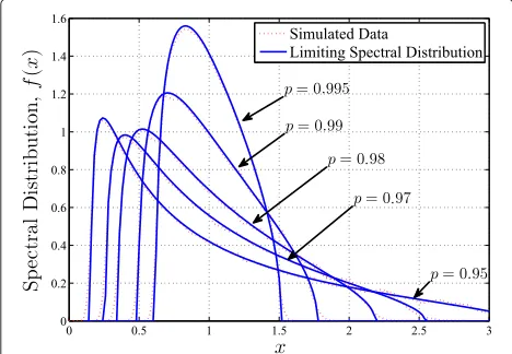
In Figure 11, the l.s.d of exponentially windowed data is plotted for different values of p ∈ {0.95, 0.97, 0.98, 0.99, 0.995}andM = 20. We observe that asptends to one, the eigenvalues become more concentrated around their true values. This is because the effective length of the window increases aspapproaches 1.

Figure 12 shows the spectral distribution for an expo-nentially windowed SCM in a case where the eigenvalues are 12, 7, 3,1 with the same multiplicity ratiosα₁= α₂= α₃ = α₄ = 1₄ for two values ofc0 = 0.1 andc0 = 0.4.

Figure 11Distribution of eigenvalues using the exponential window forM=20andp∈ {0.95, 0.97, 0.98, 0.99, 0.995}.

Figure 12Distribution of eigenvalues of exponentially windowed data forc0=0.1andc0=0.4where the covariance matrix has 4 distinct eigenvalues12,7,3,1with the same multiplicity ratiosα1=α2=α3=α4=14.

It can be seen that asc0decreases (i.e., as the forgetting

factorpincreases for a fixed value of array dimensionM) the spectral distribution tends to concentrate around the true eigenvalues. Figure 12 shows that the supports corre-sponding to eigenvaluesλ₄ =12,λ₃= 7 are not disjoint forc0=0.4 where as they are separate forc0=0.1. In this

figure, the empirical distributions are obtained using sim-ulation data withM= 20,N = −ln(γ )M_c

0 ∈ {920, 3684}

andp = e−Mc0 ∈ {0.98, 0.995} and the l.s.d. are

numer-ically calculated as introduced in the previous section. In this case the multiplicities of all of the eigenvalues of the covariance matrix is 5. We see that the l.s.d. fit the empirical results even for moderate and small array dimensions.

7 Conclusion