An image formation algorithm for missile-borne circular-scanning SAR

(1)

R E S E A R C H

Open Access

An image formation algorithm for

missile-borne circular-scanning SAR

Yesheng Gao

*

, Kaizhi Wang and Xingzhao Liu

Abstract

Circular-scanning SAR is an imaging mode with its antenna beam rotating continuously with respect to the vertical axis. An image formation algorithm for the missile-borne circular-scanning SAR is proposed in this article. Based on the principle of the polar format algorithm, the focus algorithm is generalized to form each subimage when the antenna beam scans at an arbitrary position. By calculating the 2-D position of each calibration point between the scatterers and the subimages, a method is presented to correct the geometric distortion of each subimage. This method is able to correct the geometric distortion even in the case of high maneuvering. These subimages are then mosaicked together to form a circular image. The simulation results under three diﬀerent maneuvering trajectories are given, the subimages are formed by the focusing algorithm, and then the ﬁnal circular image can be formed by mosaicking 71 subimages, each of which is after geometric distortion correction. The simulations validate the proposed image formation algorithm, and the results satisfy system design requirements.

1 Introduction

Synthetic aperture radar (SAR) is a form of radar system to provide high resolution images with the use of the rel-ative motion between the target region and the antenna, which is usually mounted on a moving platform [1-3]. The conventional platform includes aircraft, spacecraft, and satellite. The radar can also be mounted on a missile for military applications [4].

SAR system usually operates in three modes: stripmap, spotlight, and scan [1]. Circular-scanning SAR is different from these three modes, with its antenna beam rotating continuously with respect to the vertical axis [5,6]. It can provide SAR image of both sides of the flight path, and can also extend imaged area during a single pass with the same antenna. Missile-borne circular-scanning SAR suffers from complicated imaging problems: high speed, high squint angle, and high maneuvering. Sun discussed the properties of the circular-scanning SAR signal and presented an image formation algorithm based on the extended chirp scaling algorithm (ECSA) [5]. It is nature to increase the sampling rate and the memory storage for the ECSA as the squint angle increases. Li proposed a

*Correspondence: [email protected]

Department of Electronic Engineering, Shanghai Jiao Tong University, 800 Dongchuan Road, 200240, Shanghai, China

geometric-distortion correction algorithm for the succes-sive subimages formed by the linear range-Doppler algo-rithm (LRDA) [6]. LRDA is an eﬃcient image formation algorithm, but it takes extra computations to compensate for motion errors due to the high maneuvering.

We concentrate on the image formation during the mis-sile descending stage. An image formation algorithm for the missile-borne circular-scanning SAR is proposed. A processed aperture time is deﬁned as the time during which the antenna beam rotates 360 degrees. The pro-cessed aperture is divided into many subapertures, the signal of which is processed by using the principle of the polar format algorithm (PFA) [1,2]. Each subaper-ture is used to form a SAR image, namedsubimage. The focus algorithm is generalized to form each subimage when the antenna beam scans at an arbitrary position. A geometric-distortion correction method is proposed. It corrects target locations by using 2-D interpolation in image domain. This method can work even in the case of high maneuvering. The successive subimages are mosaicked together to form a circular image. Compared with the existing algorithms of the circular-scanning SAR, the proposed algorithm does not need to increase the sampling rate and memory storage when the squint angle increases. Meanwhile, there is no extra computation to

(2)

motion compensation since it is included in the subimage focusing algorithm.

The remainder of the article is organized as follows. In Section 2, the imaging geometry of the missile-borne circular-scanning SAR is introduced. In Section 3, the image formation algorithm is detailed. In Section 4, simu-lation results under three diﬀerent maneuvering trajecto-ries are described. Section 5 presents our conclusions.

2 Imaging geometry of the missile-borne circular-scanning SAR

The imaging geometry of missile-borne circular-scanning SAR is illustrated in Figure 1. Symbols are listed as follows. For clarity of the illustration, some symbols are not labeled in Figure 1.

va: velocity of the missile. Its horizontal component coincides with the positivex-axis.

H : altitude of the missile.

θ_d: dive angle which identiﬁes the direction of the missile velocity relative to the horizontal direction.

pm: the position of the antenna phase center (APC).

p_m: the corresponding nadir point ofpm.

: rotating speed of the antenna beam. It is considered positive when rotating counterclockwise.

θ_r: the angle that goes counterclockwise from the positivex-axis to the ground beam orientation. ψa: incidence angle.

βr: two-way range beamwidth.

βa: two-way azimuth beamwidth.

ϕg: projection ofβaonto thex-y plane.

α: Doppler cone angle. θgs: ground squint angle.

Otemp: temporary scene center. It coincides with the origin of the coordinate system whent=0.

Figure 1Imaging geometry of the missile-borne circular-scanning SAR.

θrchanges with time and can be expressed as

θr(t)=θr0+·t. (1)

Here, assume thatθ_r0=180◦, whent=0.

According to the imaging geometry of the missile-borne circular-scanning SAR,ϕ_gcan be expressed as

ϕ_g=2·arctan

⎡ ⎣tan βa 2

sinψa

⎤

⎦. (2)

Given the coordinate ofpm

x(t),y(t),z(t) at arbitrary timet, the size of the antenna footprint can be described as ⎧ ⎪ ⎪ ⎪ ⎪ ⎪ ⎨ ⎪ ⎪ ⎪ ⎪ ⎪ ⎩

rl(t)=z(t)·tan

ψa−

βr 2

rm(t)=z(t)·tan(ψa)

ru(t)=z(t)·tan

ψ_a+βr

2

(3)

whererm(t)is the footprint radius (distance betweenpm and Otemp), rl(t) andru(t) is the lower and upper limit radius, respectively.

Temporary scene centerOtemp

[xsc(t),ysc(t)]

is calcu-lated by ⎧ ⎨ ⎩

xsc(t)=x(t)+rm(t)·cosθr(t)

ysc(t)=y(t)+rm(t)·sinθr(t)

(4)

In particular, xsc(0),ysc(0) =[ 0, 0] according to the aforementioned assumption.

3 Image formation algorithm for the missile-borne circular-scanning SAR

The image formation algorithm for the missile-borne circular-scanning SAR is comprised of three steps: (1) subimage formation, (2) geometric-distortion correction, (3) image mosaicking. Subimages after correcting geo-metric distortion are mosaicked together to get the ﬁnal circular image. These three steps are discussed in detail in the following sections.

3.1 Subimage formation

Deﬁne

ˆ

t=t−n·Tsub (n=0, 1,. . .,N−1) (5)

whereTsubis the subaperture time,Nis the total number of the subimages. In a single subaperture time (−Tsub/2 ˆ

t < Tsub/2), the radar platform moves from the start of the subaperture to the end of the subaperture,θrchanges fromθr(tn)toθr(tn+Tsub).

(3)

ac

ψ o

temp o

x

y

z

t X

t Y

a ψ

X K

o

temp o

x

y

z

Y K r

K

p K start of the subaperture

subaperture center

end of the subaperture

trajectory

(b)

(a)

Figure 2Data collection model under high maneuvering.(a)data collection in spatial domain;(b)data collection in wavenumber domain.

the sectorθ_r can be approximated as θ_r ≈ θ_r(tn +

Tsub)−θr(tn). The lower limit ofθris determined by the required cross-range resolution of the subimages [6].

The subimage focus algorithm is generalized to process each subaperture data when the antenna beam scans at an arbitrary position, it is based on the principle of the Polar format algorithm (PFA). PFA is a typical spotlight SAR imaging algorithm [1,2,7]. It can achieve 3-D motion compensation, and the motion compensation is carried out without any extra computations [1,8]. The data collec-tion surface (DCS) is determined by the trajectory and the scene center. When the missile is highly maneuvering, the DCS is shown in Figure 2.ψais the incidence angle, and ψacis its value whenˆt=0.

In the subimage formation,x-yplane is selected as the focus target plane (FTP) and the image display plane (IDP). The signal in the DCS can be projected onto this plane. With reference to Figure 2b, the signal coordinate in the DCS can be expressed as (in wavenumber domain)

Kr= 4π

c ·f (6)

wheref is the signal frequency,cis the velocity of light. By multiplying the sine of the incidence angle sinψ_a, Equation (6) can be projected onto the FTP with

Kp=Kr·sinψa= 4π

c ·f ·sinψa. (7)

The eﬀect of maneuvering motion on the data projec-tion is illustrated in Figure 3. When the platform tra-jectory is ideal (horizontal, linear, constant velocity), the signal projection is placed as shown in Figure 3a. While the missile is highly maneuvering, the same sample of each pulse is projected to diﬀerent positions along the radial line in the FTP, as shown in Figure 3b.

Line-of-sight polar interpolation (LOSPI) is applied to the projected data. With LOSPI, the image display coor-dinates correspond to the range and cross-range coordi-nates in target space. Diﬀerentθr changes the range and cross-range direction in target space and causes the orien-tation of the imaged scene to rotate with respect to image display coordinates. Then range and cross-range IFFT are used to obtain the subimages. The ﬂowchart of the subimage formation is illustrated in Figure 4. This focus

) b ( )

a (

(4)

Raw data

Polar format

Antenna beam

position

Range

interpolation

Cross-range

interpolation

Range IFFT

Cross-rang

IFFT

Subimage

output

Figure 4Flowchart of the subimage formation.

algorithm is based on the principle of the PFA, it is gen-eralized to focus each subimage when the antenna beam scans at an arbitrary position. The resulting subimages suﬀer from the geometric distortion [1]. The geometric distortion is harmful to the image mosaicking.

3.2 Geometric-distortion correction

The geometric distortion is inevitable, its eﬀects become more evident as the resolution and the squint angle increase [9]. It is necessary to correct geometric distortion

before imaging mosaicking. Because the geometric distor-tion is spatial-variant, its correcdistor-tion must be implemented by calculating the 2-D position of each calibration point between the scatterers and the subimages [6].

The model for the geometric-distortion correction is demonstrated in Figure 5. The calibration grid is in x-y

plane and parallel to thex- andy-axes. The intervals of two adjacent calibration points arex=pxandy=py, with

pxandpydenoting the range and azimuth pixel resolution, respectively. Thext-ytcoordinate system is established as shown in Figure 5, with its origin locating at the tempo-rary scene centerOtemp. Theyt-axis indicates the ground beam orientation. Given the coordinate (x,y) in thex-y

coordinate system, its corresponding coordinate(xt,yt)in thext-ytcoordinate system can be expressed as

xt= −(x−xsc)·sinθa+(y−ysc)·cosθa

yt= −(x−xsc)·cosθa−(y−ysc)·sinθa

(8)

where θa is the angle that goes counterclockwise from the Xt-axis to theyt-axis. The Xt-Yt-Zt coordinate sys-tem is established for derivation convenience, as shown in Figure 6. The Xt-axis is perpendicular to they-axis, the

Yt-axis is perpendicular to thex-axis,Zt-axis follows the right-hand rule, the origin locates atOtemp.

In this section, we derive the position calculation of a calibration point between the scatterer and the subim-age. The derivation is in a general form and is even suited for the case of high maneuvering. Let fx(t),fy(t),fz(t) be the APC position in the x-y-z coordinate system.

fx(t),fy(t),fz(t) can be transformed into the Xt-Yt-Zt coordinate system by

⎧ ⎪ ⎨ ⎪ ⎩

FX(t)=xsc−fx(t)

FY(t)=ysc−fy(t)

FZ(t)=fz(t)

. (9)

The data coordinate in the wavenumber domain is illus-trated in Figure 7. (xp,yp) is the coordinate of the received data in the wavenumber domain, it can be expressed as

xp= −K·sin(θa−θac)

yp=K·cos(θa−θac)−Kc

(10)

where

Kc=

4πsinψac

c fc, (11)

and

K=Kc

sinψa sinψac·fc

fc+k

τ− 2Ra

c

. (12)

(5)

Figure 5Model for the geometric-distortion correction.

Assume that a calibration point locating at(TX,TY,TZ) in theXt-Yt-Ztcoordinate system, the diﬀerential range is

R=Rt−Ra

=[FX(t)−TX]2+[FY(t)−TY]2+[FZ(t)−TZ]2

−F_X2(t)+F_Y2(t)+F_Z2(t),

(13)

and the sine of the incidence angle can be expressed as

sinψa=

F_X2(t)+F_Y2(t)

Ra

(14)

whereRtis the distance from the APC to the calibration point,Ra is the distance from the APC to the temporary scene center.

After removing the residual video phase (RVP), the phase of the echo is expressed as

= −K· R

sinψa

. (15)

Using Equations (10) and (15), the Taylor series expan-sion of the phase (xp,yp) about (xp,yp) = (0, 0) is

(xp,yp)=a0+a1·xp+a2·yp+a11·x2p+a12·xp·yp

+a22·y2p+ · · ·.

(16)

x

y

temp

o

t

X

t

Y

o

t

x

t

y

a

θ

(6)

raw data

Figure 7Data coordinate in the wavenumber domain.

Here, the higher order terms are not emphasized. According to the full diﬀerential formula,a1anda2have the forms as follows

⎧ ⎪ ⎪ ⎪ ⎨ ⎪ ⎪ ⎪ ⎩

a1= ∂ ∂xp

c = ∂ ∂K ∂K ∂xp +

∂ ∂θa

∂θa ∂xp c

= − 1

Kc ∂ ∂θa c

a2= ∂ ∂yp

c = ∂ ∂K ∂K ∂yp+

∂ ∂θ_a

θa ∂yp c

= ∂ ∂K c . (17)

Equation (17) can be further written as

⎧ ⎪ ⎪ ⎨ ⎪ ⎪ ⎩

a1= − 1

Kc · dt

dθa

c ·∂ ∂t c = dt

dθa

c · R

sinψa

c

a2= −

Rc

sinψac

.

(18)

dt

dθac and

R

sinψa

cin Equation (18) can be calculated as follows.

raw data

aperture division parameters

placement in polar format

IMU/GPS range and azimuth

interpolation

set grid

coordinate calculation interpolation

scan a circle ?

output Yes No

image mosaicking range and azimuth

IFFT subimage formation correction and mosaicing

(7)

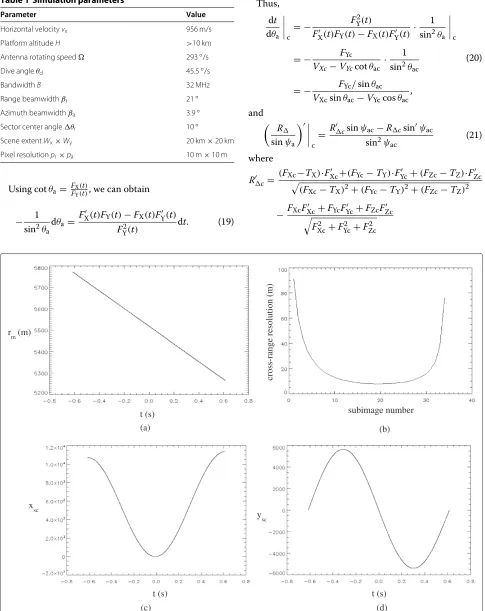
Table 1 Simulation parameters

Parameter Value

Horizontal velocityvx 956 m/s

Platform altitudeH >10 km

Antenna rotating speed 293◦/s

Dive angleθd 45.5◦/s

BandwidthB 32 MHz

Range beamwidthβr 21◦

Azimuth beamwidthβa 3.9◦

Sector center angleθr 10◦

Scene extentWx×Wy 20 km×20 km

Pixel resolutionpr×pa 10 m×10 m

Using cotθ_a= FX(t)

FY(t), we can obtain

− 1

sin2θa

dθ_a= F

X(t)FY(t)−FX(t)FY(t)

F_Y2(t) dt. (19)

Thus,

dt

dθa

c

= − FY2(t)

F_X(t)FY(t)−FX(t)FY(t)

· 1

sin2θa

c

= − FYc

VXc−VYccotθac · 1 sin2θac

= − FYc/sinθac

VXcsinθac−VYccosθac ,

(20)

and

R

sinψa

c

= Rcsinψac−Rcsinψac sin2ψac

(21)

where

Rc=

(FXc−TX)·F_Xc +(FYc−TY)·F_Yc +(FZc−TZ)·F_Zc

(FXc−TX)2+(FYc−TY)2+(FZc−TZ)2

−FXcFXc +FYcFYc +FZcF_Zc

F_Xc2 +F_Yc2 +F_Zc2

t (s) r_m(m)

subimage number

cross-rang

e resolution (m

)

(a) _(b)

t (s) t (s)

x_sc

y_sc

) d ( )

c (

(8)

= Rtc· Vac

Rtc −

Rac· Vac

Rac =

Rac− rt

· Vac

Rtc −

Rac· Vac

Rac

= −rt· Vac

Rtc −

Rc·

Rac· Vac

Rtc·Rac ,

(22)

and

sinψac=

FXcFXc +FYcFYc F2

Xc+FYc2

Rac−Rac_R· _acVac

F_Xc2 +F_Yc2

R2 ac

= VXccosθac+VYcsinθac

Rac −

sinψac

Rac Rac· Vac

Rac .

(23)

Here,Rtis the APC position vector relative to the cali-bration point,Rais the APC position vector relative to the temporary scene center,rtis the calibration point position vector relative to the temporary scene center. Vac is the velocity vector in theXt-Yt-Ztcoordinate system,VXcand

VYc are its components in theXt- andYt-axes. The sub-scriptcrefers to the values of the corresponding variables at the subaperture center.

The position of a calibration point in the correspond-ing subimage is derived. Given a calibration point locat-ing at (x,y) in the x-ycoordinate system (a ﬂat earth is assumed), its corresponding position in the subimage can be obtained by

⎧ ⎪ ⎪ ⎪ ⎪ ⎨ ⎪ ⎪ ⎪ ⎪ ⎩

Na= −

a1

pa +

NaFFT 2

Nr= −

a2

pr +

NrFFT 2

(24)

where pr = ₂_Bc_r_NN_rFFTrout, pa = ₂_Bc_a_NN_aFFTaout. Br and Ba are range and azimuth output bandwidth,Nxoutis the sample number of the interpolation output in the range/azimuth direction,NxFFTis the FFT size.

Specially, we present the form of equation (18) under vertical maneuvering. That is, only the vertical compo-nent ofvais changing with time, its horizontal component is a constant. This is due to the fact that the impact of the

) c ( )

b ( )

a (

(d) (e) (f)

(9)

Figure 11IPRs of three point targets, whenθr=90◦.IPRs analysis when the vertical velocity is constant (θr=90◦). The results of three diﬀerent point targets are given.(a)Target of the nearest distance;(b)target of the middle distance;(c)target of the farthest distance.

vertical maneuvering is serious to the circular-scanning SAR, and the vertical maneuvering is used in the following simulation experiments.

a1=xp−

1

2Rac·sinθac·sinψac

cosθ_ac·sin2ψ_ac·y2_p

×1+2 sin2ψ_ac −2 sin2ψ_ac·TX·yp−cosθac·r2t

−VZc·sin2ψac·cosψac

Rac·VXc·sinθac ·

y2_p,

(25)

and

a2=yp− 1 2Rac·sinψac

r2_t −sin2ψ_ac·y2_p. (26)

Here, Ra is the distance between the APC and the temporary scene center. rt is the distance between the

Table 2 PSLRs analysis of the IPRs (vertical velocity is constant)

PSLR of range IPR PSLR of cross-range IPR

Nearest target −12.04 dB −13.03 dB

Middle target −13.28 dB −13.23 dB

(10)

temporary scene center and the calibration point.TX is the coordinate of the calibration point in theXt-axis,VZis the component ofvain theZt-axis,VXin theXt-axis, these variables are evaluated in theXt-Ytcoordinate system.θac, ψac,Vxc,Vzc, andRacare the values of the corresponding variables at the subaperture center.

The geometric distortion can be corrected as follows.

Step 1: Set calibration grid, as shown in Figure 5.

Step 2: Calculate the position of each calibration point in the subimage,(Nr,Na). These calibration points are constrained within the instantaneous imaging area.

Step 3: Obtain the intensity of the corresponding position via 2-D interpolation.

3.3 Image mosaicking

Subimages are focused as discussed in Section 3.1. The method proposed in Section 3.2 can correct their

geo-metric distortion. The ﬁnal circular image is formed by mosaicking together these subimages. The image mosaicking can be described as follows.

Step 1: Calculate the size of the ﬁnal output image, allocate a matrix to store the image. The complete illuminated area (0◦θr<360◦) can be calculated according to the radar system parameters. Thus, the size of the output image can be determined whenpr andpaare known. It should be noted that each pixel in the output image corresponds to a calibration point.

Step 2: Correct the geometric distortion of each calibration point in the temporary illuminated area. The temporary illuminated area can be calculated using the radar system parameters, the instantaneous radar platform position and the value ofθr. The geometric distortion of each calibration point in this area can be corrected by using the method described

(11)

in Section 3.2. Then the subimage without geometric distortion is stored into the positions where the calibration points are located.

Step 3: If all the subimages are formed (in the later simulations, the number of subimages to constitute a circular image is 71), output the ﬁnal circular image. Otherwise, return to Step 2 to form the next subimage. Thus, the ﬁnal circular image can be formed by adding successive subimages.

The geometric distortion is corrected point-by-point, the successive subimages are mosaicked together to form the final circular image. This can well describe the circular-scanning SAR imaging procedure. Note that not only the final circular image can be formed, but the image with the beam rotating at an arbitrary position can be produced. The final image product and the intermedi-ate result are stored in the same matrix, which reduces the memory requirement and computational complex-ity. The image formation algorithm for the missile-borne circular-scanning SAR is demonstrated in Figure 8.

3.4 Computational consideration

The image formation algorithm of the missile-borne circular-scanning SAR is detailed in the three preced-ing sections. This algorithm is comprised of three steps: subimage formation, geometric-distortion correction, and image mosaicking. In the subimage formation, the major computational burden is the interpolation and the IFFT operation. The computational complexity of the interpo-lation operation can be expressed as

CP=0.4·Lout[(Lf−1)rDS+1]Mk (27)

whereLoutis the output length of the interpolation,Lfis the length of the ﬁlter,rDSis the downsampling ratio,Mk is a constant and its typical value is 1.25 [1]. The inter-polation can also be implemented by chirp z-transform [9]. The lengths of IFFT operation are Nrout and Naout in the range and cross-range direction, respectively. After position calculation, the geometric-distortion correction is implemented by interpolation operation, the compu-tational complexity can be determined by Equation (27).

(12)

Figure 14IPRs of three point targets, whenθr=90◦.IPRs analysis when the vertical velocity is uniformly accelerated (θr=90◦). The results of three diﬀerent point targets are given.(a)Target of the nearest distance;(b)target of the middle distance;(c)target of the farthest distance.

Image mosaicking is separated as the third step, but its realization is included in geometric-distortion correction and no extra computation is needed.

4 Simulation results

To validate the performance of the proposed algorithm, simulation results under three diﬀerent maneuvering motions are presented. The primary parameters of a Ku-band radar system are given in [6] and are listed in Table 1. In Section 4.1, the vertical velocityvz does not change with time, and the horizontal velocityvxis also constant. To validate the image formation algorithm in subimage formation and geometric-distortion correction, the simu-lated point targets are placed as a rectangle with the size of 11×15, the distance between two adjacent targets is 200 m. The characteristics of the imaged area (footprint radius, and coordinates of the temporary scene center) and the cross-range resolution of successive subimages are analyzed. Three subimages and their geometric-distortion correction results are given. Quantitative analysis of the result is also given.

In Section 4.2, the horizontal velocity is still constant, the vertical velocity is uniformly accelerated. The point targets are placed the same as those in Section 4.1. The characteristics of imaged area, the cross-range resolution of successive subimages, and three typical subimages are given. Quantitative analysis of the result is also given.

In Section 4.3, the horizontal velocity is still constant, the vertical velocity changes with time in sinusoidal form. In this section, the ﬁnal circular image is give. The ground point targets are placed uniformly with the interval of 200 m× 200 m, the total number of the targets is 95× 95. The cross-range resolution of successive subimages are illustrated.

Table 3 PSLRs analysis of the IPRs (vertical velocity is uniformly accelerated)

PSLR of range IPR PSLR of cross-range IPR

Nearest target −13.11 dB −11.54 dB

Middle target −13.25 dB −13.13 dB

(13)

The major computations involved in the image forma-tion algorithm are interpolaforma-tion and IFFT, both operaforma-tions are applied in the range and azimuth directions. In the range direction, the value ofLoutis 2048,Lfis 8,rDSis 1. In the azimuth direction,Loutis 340,Lfis 8,rDSis 1.51. The IFFT size in range is 2048, azimuth 512.

4.1 Constant velocity in the vertical direction

Vertical velocityvzis set at−973 m/s. The footprint radius is shown in Figure 9a, its value decreases gradually due to the platform altitude reduction. The coordinate of the temporary scene center is illustrated in Figure 9c,d, respectively. Figure 9b shows the cross-range resolution (0◦ θ_r 180◦). The resolution decreases as the squint angle increases, the ﬁnest resolution can be achieved whenθr=90◦orθr=270◦.

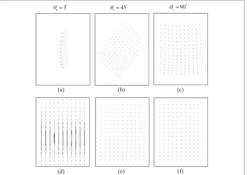
The subimages of three typical values ofθrare shown in Figure 10. Figure 10a–c are the subimages whenθr =5◦,

45◦, and 90◦. The geometric distortion is evident in these subimages, especially in Figure 10a,b. Because LOSPI is applied, the received data at diﬀerent look angles change the range and cross-range directions in target space. The orientation of the resultant subimage rotates with respect to the image display coordinates. Figure 10d–f are the geometric-distortion correction results. Although the geometric distortion is corrected, it is also diﬃcult to distinguish targets in cross-range direction in Figure 10d since θ_r is around 0◦. It is the inevitable drawback of side-look SAR to distinguish targets at the forward and backward directions [1].

The impulse responses (IPRs) of three point targets at diﬀerent distances are given in Figure 11. The three tar-gets locate at the nearest, middle, and farthest distances from the APC. With reference to Figure 11, the peak side-lobe ratio (PSLRs) of range IPRs and cross-range IPRs are analyzed, as given in Table 2 (no windowing functions are

(14)

Figure 16Locations of the illuminated point targets.

used). The point targets located in these three diﬀerent distances are well focused.

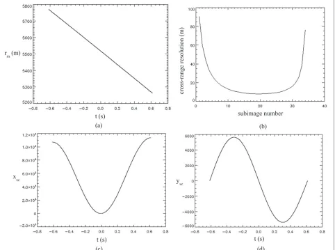
4.2 Uniformly acceleration in the vertical direction

The vertical velocity is set in the form ofvz = vz0+azt, withvz0= −973 m/s andaz= −10 m/s2. Whenθrrotates from 0◦to 360◦, the change of the footprint radius rm is illustrated in Figure 12a. The cross-range resolution of successive subimages are shown in Figure 12b, only the part withθ_r changing from 0◦to 180◦ is shown due to the symmetry. The coordinates of temporary scene cen-ter as shown in Figure 12c,d correspond withθ_r, they can indicate the imaged area.

Three subimages and their corresponding geometric-distortion correction results are shown in Figure 13. Figure 13a–c are the subimages when θr = 5◦, 45◦, and 90◦, the results of geometric-distortion correction are illustrated in Figure 13d–f. The geometric distortion in the subimages is obvious. These image products do not meet the application and mosaicking requirements. The geometric distortion is then corrected and the positions of the point targets are identical to their assumed positions. The simulation results show that the proposed image for-mation algorithm can form subimages without geometric distortion even under the high maneuvering motions.

The impulse responses (IPRs) of three point targets at diﬀerent distances are given in Figure 14. With reference to Figure 14, the peak sidelobe ratio (PSLR)s of range IPRs and cross-range IPRs are analyzed, as given in Table 3 (no windowing functions are used). The IPRs analysis demon-strates that the targets located in the whole illuminated area can be well focused, and the performance meets the system requirement.

Figure 17Imaging result of missile-borne circular-scanning SAR.

4.3 Vertical velocity changes with time in sinusoidal form

In the 3rd condition, vertical velocity has the form of

vz=vz0+2π·fz·Az·cos(2πfzt), wherevz0= −973 m/s,

fz= 5 Hz,Az=15 m. The trajectory perturbation in ver-tical direction is studied in this simulation, and the motion parameters are set according to [10]. The footprint radius decreases as the platform altitude decreases, as shown in Figure 15a. Diﬀerent subimages have diﬀerent cross-range resolution, as shown in Figure 15b, the minimum value is about 10 m. The antenna beam pointing changes withθ_r, the coordinates of temporary scene center are illustrated in Figure 15c,d.

Withθrrotating from 0◦to 360◦, the locations of the illuminated point targets are illustrated in Figure 16. The annular shape is determined by the radar system and the platform motion. The imaging result of the missile-borne circular-scanning SAR is shown in Figure 17. The complete circular image is obtained by mosaicking 71 suc-cessive subimages. In Figure 17, the point targets are uni-formly distributed, their positions are identical to those shown in Figure 16. It is interesting that the targets locat-ing at the forward and backward directions cannot be distinguished. It is due to the fact that the contour lines of the iso-range and iso-Doppler circles are nominally paral-lel in these two directions, suggesting that the inability of range-Doppler discrimination to position ground echoes.

5 Conclusion

(15)

Simulation results under three different maneuvering motions are given, each point target in the illuminated area is well focused, the geometric distortion is corrected using the method presented in Section 3.2, and the final circular image can be generated through image mosaick-ing. From the simulation results done so far, we are con-fident that the image formation algorithm is stable and effective for missile-borne circular-scanning SAR, even under highly maneuvering conditions. Our further study will focus on the impact of assuming the wrong calibration point height, and more precise geometric-distortion cor-rection method by using an external DEM. Motion errors and factors which deteriorate the image quality will also be our further study.

Competing interests

The authors declare that they have no competing interests.

Acknowledgements

The authors wish to thank Dr. Daiyin Zhu from Nanjing University of Aeronautics and Astronautics for helpful technical discussions.

Received: 11 August 2012 Accepted: 7 December 2012 Published: 2 January 2013

References

1. WG Carrara, RM Majewski, RS Goodman,Spotlight Synthetic Aperture Radar: Signal Processing Algorithms, (Artech House, Norwood, 1995)

2. DE Wahl, PH Eichel, DC Ghiglia, PA Thompson, CV Jakowatz, Spotlight-Mode Synthetic Aperture Radar: A Signal Processing Approach. (Kluwer Academic Publishers, Boston, 1996)

3. IG Cumming, FH Wong,Digital Processing of Synthetic Aperture Radar Data: Algorithms and Implementation, (Artech House, Norwood, 2005) 4. B Deng, X Li, H Wang, Y Qin, J Wang, Fast raw-signal simulation of

extended scenes for missile-borne SAR with constant acceleration. IEEE Geosci. Rem. Sens. Lett.8, 44–48 (2011)

5. B Sun, Y Zhou, T Li, J Chen, in2006 International Conference on Radar, vol. 1. Image formation algorithm for the implementation of circular scanning, SAR, (Shanghai, 2006), pp. 1–4

6. Y Li, D Zhu, The geometric-distortion correction algorithm for circular-scanning SAR imaging. IEEE Geosci. Rem. Sens. Lett.7, 376–380 (2010)

7. B Rigling, R Moses, Taylor expansion of the diﬀerential range for monostatic SAR. IEEE Trans. Aerosp. Electron. Syst.41, 60–64 (2005) 8. D Zhu, Z Zhu, Range resampling in the polar format algorithm for

spotlight SAR image formation using the chirp z-Transform. IEEE Trans. Signal Process.55, 1011–1023 (2007)

9. D Zhu, Y Li, Z Zhu, A keystone transform without interpolation for SAR ground moving-target imaging. IEEE Geosci. Rem. Sens. Lett.4, 18–22 (2007)

10. G Fornaro, Trajectory deviations in airborne SAR: analysis and compensation. IEEE Trans. Aerosp. Electron. Syst.35, 997–1009 (1999)

doi:10.1186/1687-6180-2013-2

Cite this article as:Gaoet al.:An image formation algorithm for missile-borne circular-scanning SAR.EURASIP Journal on Advances in Signal Processing 20132013:2.