Target detection performance bounds in compressive imaging

R E S E A R C H

Open Access

Target detection performance bounds in

compressive imaging

Kalyani Krishnamurthy

, Rebecca Willett

and Maxim Raginsky

Abstract

This article describes computationally efficient approaches and associated theoretical performance guarantees for the detection of known targets and anomalies from few projection measurements of the underlying signals. The

proposed approaches accommodate signals of different strengths contaminated by a colored Gaussian background, and perform detection without reconstructing the underlying signals from the observations. The theoretical

performance bounds of the target detector highlight fundamental tradeoffs among the number of measurements collected, amount of background signal present, signal-to-noise ratio, and similarity among potential targets coming from a known dictionary. The anomaly detector is designed to control the number of false discoveries. The proposed approach does not depend on a known sparse representation of targets; rather, the theoretical performance bounds exploit the structure of a known dictionary of targets and the distance preservation property of the measurement matrix. Simulation experiments illustrate the practicality and effectiveness of the proposed approaches.

Keywords: Target detection, Anomaly detection, False discovery rate,p-value, Incoherent projections, Compressive sensing

Introduction

The theory of compressive sensing (CS) has shown that it is possible to accuratelyreconstructa sparse signal from few (relative to the signal dimension) projection measure-ments [1,2]. Though such a reconstruction is crucial to visually inspect the signal, there are many instances where one is solely interested in identifying whether the under-lying signal is one of several possible signals of interest. In such situations, a complete reconstruction is computa-tionally expensive and does not optimize the correct per-formance metric. Recently, CS ideas have been exploited in [3-5] to perform target detection and classification from projection measurements, without reconstructing the underlying signal of interest. In [3,5], the authors pro-pose nearest-neighbor based methods to classify a signal

f ∈RN _{to one ofmknown signals given projection} mea-surements of the formy = Af +n ∈ RK forK ≤ N, where A ∈ RK×N is a known projection operator and

n∼N0,σ2Iis the additive Gaussian noise. This model is simple to analyze, but is impractical, since in reality, a

*Correspondence: [email protected]

1Department of Electrical and Computer Engineering, Duke University, Durham, NC 27708, USA

Full list of author information is available at the end of the article

signal is always corrupted by some kind of interference or background noise. Extension of the methods in [3,5] to handle background noise is nontrivial. Though, Duarte et al. [4] provides a way to account for background con-tamination, it makes a strong assumption that the signal of interest and the background are sparse in bases that are incoherent. This might not always be true in many applications. Recent works on CS [6,7] allow for the input signalf to be corrupted by some pre-measurement noise

b∼N0,σ_b2Isuch that one observesy=A(f +b)+n, and study reconstruction performance as a function of the number of measurements, pre- and post-measurement noise statistics and the dimension of the input signal. In this work, however, we are interested in performing target detection without an intermediate reconstruction step. Furthermore, the increased utility of high-dimensional imaging techniques such as spectral imaging or videog-raphy in applications like remote sensing, biomedical imaging and astronomical imaging [8-15] necessitates the extension of compressive target detection ideas to such imaging modalities to achieve reliable target detec-tion from fewer measurements relative to the ambient signal dimensions.

For example, recent advances in CS have led to the development of new spectral imaging platforms which attempt to address challenges in conventional imaging platforms related to system size, resolution, and noise by acquiring fewer compressive measurements than spa-tiospectral voxels [16-21]. However, these system designs have a number of degrees of freedom which influence subsequent data analysis. For instance, the single-shot compressive spectral imager discussed in [18] collectsone coded projection of each spectrum in the scene. One projection per spectrum is sufficient for reconstructing spatially homogeneous spectral images, since projections of neighboring locations can be combined to infer each spectrum. Significantly more projections are required for detecting targets of unknown strengths without the ben-efit of spatial homogeneity. We are interested in investi-gating how several such systems can be used inparallel to reliably detect spectral targets and anomalies from different coded projections.

In general, we consider a broadly applicable framework that allows us to account for background and sensor noise, and perform target detection directly from projection measurements of signals obtained at different spatial or temporal locations. The precise problem formulation is provided below.

Problem formulation

Let us assume access to a dictionary of possible targets of interestD = {f(1),f(2),. . .,f(m)}, wheref(j) ∈ RN for j = 1,. . .,mis unit-norm. Our measurements are of the form

zi=Φ(αifi∗+bi)+wi (1)

where

• i∈ {1,. . .,M}indexes the spatial or temporal locations at which data are collected;

• αi≥0is a measure of the signal-to-noise ratio at locationi, which is either known or estimated from observations;

• Φ∈RK×N_{forK<N, is a measurement matrix to} be specified in Section “Whitening compressive observations”;

• bi∈RN ∼N(μb,Σb)is the background noise vector, andwi∈RK ∼N(0,σ2I)is the i.i.d. sensor noise.

For example, in the case of spectral imaging f∗_i repre-sents the spectrum at the ith spatial location, and in video sequencesf∗_i represents the vectorized image frame obtained at theith time interval. In this article we consider the following target detection problems:

(1) Dictionary signal detection (DSD): Here we assume that eachf∗_i ∈Dfori∈ {1,. . .,M}, and our task is

to detect all instances of one target signalf(j)∈D for some unknownj∈ {1,. . .,m}, i.e., to locate S=i:f∗_i =f(j). DSD is useful in contexts in which we know the makeup of a scene and wish to focus our attention on the locations of a particular signal. For instance, in spectral imaging, DSD is used to study a scene of interest by classifying every spectrum in the scene to different known classes [11,22]. In a video setup, DSD could be used to classify video segments to one of several categories (such as news, weather, sports, etc.) by projecting the video sequence to an appropriate feature space and comparing the feature vectors to the ones in a known dictionary [23].

(2) Anomalous signal detection (ASD): Here, our task is to detect all signals which arenot members of our dictionary, i.e., detectS=i:f∗_i ∈/D(this is akin to anomaly detection methods in the literature which are based on nominal, nonanomalous training samples [24,25]). For instance, ASD may be used when we know most components of a spectral image and wish to identify all spectra which deviate from this model [26].

Our goal is to accurately perform DSD or ASD with-out reconstructing the spectral input f∗_i fromzi fori ∈ {1,. . .,M}. Accounting for background is a crucial issue. Typically, the background corresponding to the scene of interest and the sensor noise are modeled together by a colored multivariate Gaussian distribution [27]. However, in our case, it is important to distinguish the two because of the presence of the projection operator Φ. The pro-jection operator acts upon the background spectrum in the same way as on the target spectrum, but it does not affect the sensor noise. We assume that bi and wi are independent of each other, and the prior probabilities of different targets in the dictionaryp(j) _=Pf∗

i =f(j) for j∈ {1,· · ·,m}are known in advance. If these probabilities are unknown, then the targets can be considered equally likely. Given this setup, our goal is to develop suitable target and anomaly detection approaches, and provide theoretical guarantees on their performances.

on an automatic detection algorithm. However, using this intermediate step has two potential pitfalls. First, the Rao– Blackwell theorem [28] tells us that an optimal detection algorithm operating on the processed data (i.e., not suf-ficient statistics)cannot perform better than an optimal detection algorithm operating on the raw data. In other words, optimal performance is possible on the raw data, but we have no such performance guarantee for the structed signals. Second, the relationship between recon-struction errors and detection performance is not well understood in many settings. Although we do not recon-struct the underlying signals, our performance bounds are intimately related to the signal resolution needed to achieve the signal diversity present in our dictionary. Since we have many fewer observations than the signals at this resolution, we adopt the “compressive” terminology.

Performance metric

To assess the performance of our detection strategies, we consider the false discovery rate (FDR) metric and related quantities developed for multiple hypothesis testing prob-lems [29]. Since we collectMindependent observations of potentially different signals, we are simultaneously con-ductingMhypothesis tests when we search for targets. Unlike the probability of false alarm, which measures the probability of falsely declaring a target for a singletest, the FDR measures the fraction of declared targets that are false alarms, that is, it provides information about the entire set ofMhypotheses instead of just one. More formally, the FDR is given by,

FDR=E

V

R

,

whereV is the number of falsely rejected null hypothe-ses, andRis the total number of rejected null hypothe-ses. Controlling the FDR in a multiple hypothesis testing framework is akin to designing a constant false alarm rate (CFAR) detector in spectral target detection applications that keeps the false alarm rate at a desired level irre-spective of the background interference and sensor noise statistics [22].

Previous investigations

Much of the classical target detection literature [30-34] assume that each target lies in aP-dimensional subspace ofRN forP<N. The subspace in which the target lies is often assumed to be known or specified by the user, and the variability of the background is modeled using a prob-ability distribution. Given knowledge of the target sub-space, background statistics and sensor noise statistics, detection methods based on LRTs (likelihood ratio tests) and GLRTs (generalized likelihood ratio tests) have been

proposed in [30-35]. A subspace model is optimal if the subspace in which targets lie is known in advance. How-ever, in many applications, such subspaces might be hard to characterize. An alternative, and a more flexible option is to assume that the high-dimensional target exhibits some low-dimensional structure that can be exploited to perform efficient target detection. This approach is uti-lized in this work and in [5] where the target signal inRN is assumed to come from a dictionary of mknown sig-nals such thatm N, and in [3], where the targets are assumed to lie in a low-dimensional manifold embedded in high-dimensional target space.

consider compressive classification performance for a singlehypothesis test.

The authors of a more recent work [38] extend the classical RX anomaly detector [39] to directly detect anomalies from random, orthonormal projection mea-surements without an intermediate reconstruction step. They numerically show how the detection probability improves as a function of the signal-to-noise ratio when the number of measurements changes. Though proba-bility of detection is a good performance measure, in many applications controlling the false discoveries below a desired level is more crucial. As a result, in our work, we propose an anomaly detection method that controls the FDR below a desired level.

Contributions

This article makes the following contributions to the above literature:

• Acompressive target detection approach, which (a) is computationally efficient, (b) allows for the signal strengths of the targets to vary with spatial location, (c) allows for backgrounds mixed with potential targets, (d) considers targets with different a priori probabilities, and (e) yields theoretical guarantees on detector performance. This article unifies preliminary work by the authors [40,41], presents previously unpublished aspects of the proofs, and contains updated experimental results.

• A computationally efficientanomaly detection method that detects anomalies of different strengths from projection measurements and also controls the FDR at a desired level.

• Awhitening filter approach to compressive measurements of signals with background contamination, and associated analysis leading to bounds on the amount of background to which our detection procedure is robust.

The above theoretical results, which are the main focus of this article, are supported with simulation studies in Section “Experimental results”. Classical detection meth-ods described in [22,26,27,30-35,39,42-45] do not estab-lish performance bounds as a function of signal resolution or target dictionary properties and rely on relativelydirect observationmodels which we show to be suboptimal when the detector size is limited. The methods in [3,4] do not contain performance analysis, and our analysis builds upon the analysis in [5] to account for several specific aspects of the compressive target detection problem.

Whitening compressive observations

Before we present our detection methods for DSD and ASD problems, respectively, we briefly discuss a whitening step that is common to both our problems of interest.

Let us suppose that there are enough background train-ing data available to estimate the background mean μb and covariance matrix Σb. We can assume without loss of generality thatμ_b = 0sinceΦμ_b can be subtracted from y. Given the knowledge of the background statis-tics, we can transform the background and sensor noise model Φbi +wi ∼ N(0,ΦΣbΦT + σ2I) discussed in (1) to a simple white Gaussian noise model by multiplying the observationszi,i∈ {1,. . .,M}, by thewhitening filter CΦ (ΦΣbΦT+σ2I)−1/2. This whitening transforma-tion reduces the observatransforma-tion model in (1) to

y_i=CΦΦαif∗i +bi

+wi

zi

=αiAf∗i +ni (2)

where

A=CΦΦ, (3)

andni = CΦ(Φbi+wi) ∼ N(0,I). To verify thatni ∼ N(0,I), observe that

ni=CΦ(Φbi+wi)∼N ⎛ ⎜ ⎜ ⎝0,CΦ

ΦΣbΦT_+σ2_{I C}T

Φ

I

⎞ ⎟ ⎟ ⎠.

We can now choose Φ so that the correspondingAhas certain desirable properties as detailed in Sections “Dic-tionary signal detection” and “Anomalous signal detec-tion”.

For a given A, the following theorem provides a con-struction of Φ that satisfies (3) and a bound on the maximum tolerable background contamination:

Theorem 1.LetB = I−AΣbAT. If the largest

eigen-value ofΣbsatisfies

λmax< 1

A2, (4)

whereAis the spectral norm ofA, thenBis positive def-inite and Φ = σB−1/2Ais a sensing matrix, which can be used in conjunction with a whitening filter to produce observations modeled in (2).

changing background statistics and other operating con-ditions.

In the sections that follow, we consider collecting mea-surements of the formy_i=αiAf∗i +nigiven in (2), where

f∗_i is the target of interest fori=1,. . .,M, andA∈RK×N is a sensing matrix that satisfies (3). It is assumed that any background contamination has been eliminated with the whitening procedure described in this section.

Dictionary signal detection

Suppose that the end user wants to test for the presence of one known target versus the rest, but it is not known a priori which target fromDthe user wants to detect. In this case, let us cast the DSD problem as a multiple hypothesis testing problem of the form

H(j)

0i :f∗i =f(j) vs. H

(j)

1i :f∗i =f(j) (5)

wheref(j)∈Dis the target of interest andi=1,. . .,M.

Decision rule

We define our decision rule corresponding to target

f(j)_{∈Din terms of a set of significance regionsΓ}(j)

i such

that one rejects theith null hypothesis if its test statistic

y_i falls in theith significance region. Specifically, Γ_i(j) is defined according to

Γ(j)

i =

y: logPf∗_i =f(j)y_i,αi,A ≤ (6)

logP

f∗_i =f()y_i,αi,A for some∈ {1,. . .,m}, =j

,

where logPf∗_i=f(j)y_i,αi,A = K₂ log ₁

2π

−

yi−αiAf(j)

2

2 + logp(j) is the logarithm of the a posteri-ori probability density of the targetf(j)at theith spatial location given the observations y_i, the signal-to-noise ratioαi and the sensing matrix A, andp(j) is the a pri-ori probability of target classj. Note that the process of determining these decision regions involves a sequence of nearest-neighbor calculations, so the computational com-plexity scales with the number of classesm. In this work, we operate under the assumption thatmis much smaller than the dimensionality of the datasets we consider. For example, if we consider spectral images, then the number of objects (signal classes) that make up a scene of interest is often smaller than the number of voxels in the image. This assumption is not unrealistic and has been exploited in earlier work such as [22] and the references therein. In most of the prior work we have surveyed [46,47], the number of signal classes is less than 35, which doesn’t make our approach intractable.

The decision rule can be formally expressed in terms of the significance regions as follows:

rejectH(_0ij)if the test statisticy_i∈Γ_i(j). (7)

We analyze this detector by extending the positive FDR (pFDR) error measure introduced by Storey to character-ize the errors encountered in performing multiple, inde-pendent andnonidenticalhypothesis tests simultaneously [48]. The pFDR, discussed formally below, is the fraction of falsely rejected null hypotheses among the total num-ber of rejected null hypotheses, subject to the positivity condition that one rejects at least one null hypothesis. The pFDR is similar to the FDR except that the positivity condition is enforced here. In our context, the positivity condition means that we declare at least one signal to be a nontarget, which in turn implies that the scene of interest is composed of more than one object in the case of spec-tral imaging, or that the scene is not static in the case of video imaging.

Consider a collection of significance regions Γ =

Γi(j):i=1,· · ·,M

, such that one declares H(_1ij) if the

test statistic y_i ∈ Γ_i(j). The pFDR for multiple, non-identicalhypothesis tests can be defined in terms of the significance regions as follows:

pFDR(j)(Γ) = E

V(Γ) R(Γ)

R(Γ) >0

(8)

where

V(Γ)= M

i=1 I

yi∈Γ( j)

i

_I{

H0i} (9)

is the number of falsely rejected null hypotheses,

R(Γ)= M

i=1 I

yi∈Γ( j)

i

₍₁₀₎

is the total number of rejected null hypotheses, and I{E} = 1 if eventEis true and 0 otherwise. In our setup,

the pFDR corresponds to the expected ratio of the num-ber of missed targets to the numnum-ber of signals declared to be nontargets subject to the condition that at least one signal is declared to be a nontarget (note that this ratio is traditionally referred to as the positive false nondis-covery rate (pFNR), but is technically the pFDR in this context because of our definitions of the null and alternate hypotheses). The theorem below presents our main result:

Theorem 2.Given observations of the form (2), if

(7), then the worst-case pFDR given by pFDR_max = maxj∈{1,...,m}pFDR(j)(Γ),satisfies the following bound:

pFDR_max≤min

1, (Pe)max 1−pmax−(Pe)max

(11)

where

pmax= max j∈{1,...,m}p

(j)_,

(Pe)max= max i∈{1,...,M}P

f_i =f∗_i , and

f_i =arg max

f∈D P

f∗_i =fy_i,αi,A. (12)

The proof of this theorem is detailed in Appendix 2. A key element of our proof is the adaptation of the tech-niques from [48] tononidenticalindependent hypothesis tests.

An achievable bound on the worst-case pFDR

Theorem 2 in the preceding section shows that, for a given

A, the worst-case pFDR is bounded from above by a func-tion of the worst-case misclassificafunc-tion probability. In this section, we use this theorem to establish an achievable bound on the worst-case pFDR that explicitly depends on the number of observations K, signal strengths {αi}Mi=1, similarity among different targets of interest, and a priori target probabilities.

Let us first define the quantities

dmin= min

f(i)_,f(j)_{∈D,i =j}f

(i)_−f(j)

pmin= min j∈{1,...,m}p

(j)

αmin= min i∈{1,...,M}αi.

Then we have the following theorem, whose proof is given in Appendix 3:

Theorem 3.Let λmax denote the largest eigenvalue of

Σb. For a given0< < 1−pmax, assume that K and N are sufficiently large so that the following conditions hold:

1−pmax− ≥ 1−pmin pmin

1+αmin 2_d2

min 4Kσ2

−K

2

+2 exp

−(K+N)2 2

(13a)

λmax<

1

(1+)2

N K +1

2, (13b)

K >

2 log_p2

min

1−pmin

1−pmax

log

1+ α

2 mind2min

4K

. (13c)

Then there exists a K×N sensing matrixAthat satisfies the condition of Theorem 1, and for which

pFDR_max≤ 1

pmin

⎛ ⎝1−pmax

1−pmin

1+α 2 mind2min

4K

K

2

− 1

pmin

⎞ ⎠ −1

+2(1−pmax)

2 exp

−(K+N)2

2

. (14)

This result has the following implications and conse-quences:

(1) For a givenN, the upper bound (13b) onλmax increases asK increases, which implies that the system can tolerate more background perturbation if we collect more measurements.

(2) The pFDR bound (14) decays with the increase in the values ofK,dminandαmin, and increases aspmin decreases. For a fixedpmax,pmin,αminanddmin, the bound in (14) enables one to choose a value ofK to guarantee a desired pFDR value.

(3) The dominant part of the bound (14) is independent ofN, and is only a function of K,pmax,pmin,αmin, anddmin. The lack of dependence onN is not unexpected. Indeed, when we are interested in preserving pairwise distances among the members of a fixed dictionary of sizem, the

Johnson–Lindenstrauss lemma [49] says that, with high probability,K=Ologmrandom Gaussian projections suffice, regardless of the ambient dimensionN. This is precisely the regime we are working with here.

(4) The bound onK given in (13c) increases

logarithmically with the increase in the difference betweenpmaxandpmin. This is to be expected since one would need more measurements to detect a less probable target as our decision rule weights each target by itsa priori probability. If all targets are equally likely, thenpmax=pmin=1/m, and K=Ologmis sufficient providedα2_mind2_minis sufficiently large such that

log

1+α 2 mind2min

4K

> log

1+ α 2 mind2min

4N

>1

(where the first inequality holds sinceK<N). In addition, the lower bound onK also illustrates the interplay between the signal strength of the targets, the similarity among different targets inD, and the number of measurements collected. A small value of dminsuggests that the targets inDare very similar to each other, and thusαminandK need to be high enough so that similar targets can still be

Section “Experimental results” illustrate the tightness of the theoretical results discussed here.

Inspection of the proof shows that if A is generated according to a Gaussian distribution, then the conditions of Theorem 3 will be met with high probability.

Extension to a manifold-based target detection framework

The DSD problem formulation in Section “ASD problem formulation” is accurate if the signals in the dictionary are faithful representations of the target signals that we observe. In reality, however, the target signals will dif-fer from the dictionary signals owing to the differences in the experimental conditions under which they are col-lected. For instance, in spectral imaging applications, the observed spectrum of any material will not match the reference spectrum of the same material observed in a laboratory because of the differences in atmospheric and illumination conditions. To overcome this problem, one could form a large dictionary to account for such uncer-tainties in the target signals and perform target detec-tion according to the approaches discussed in Secdetec-tions “Whitening compressive observations” and “Dictionary signal detection”. A potential drawback with this approach is that our theoretical performance bound increases with the size ofDthrough pmin anddmin. Instead, one could reasonably model the target signals observed under dif-ferent experimental conditions to lie in a low-dimensional submanifold of the high-dimensional ambient signal space as shown to be true for spectral images in [50]. We can exploit this result to extend our analysis to a much broader framework that accounts for uncertainties in our dictionary.

Let us consider a dictionary of manifolds DM =

M(1)_{,. . .,M}(m) _{corresponding to m different target} classes, and thatf∗_i fori∈ {1,. . .,M}is in one of the man-ifolds inD_M. Considering an observation model of the form given in (2), our goal is to determinei:f∗_i ∈M(j), where j ∈ {1,. . .,m} is the target class of interest. Let us assume that all target classes are equally likely to keep the presentation simple, though the analysis extends to the case where the targets classes have different a priori probabilities. Suppose that we collect independent sets of measurementsy_iM_i=1andy_iM_i=1. Then, we can use the following two-step procedure to extend our DSD method to this manifold-based framework:

(1) Giveny_i, form a data-dependent dictionary Dy_i=

f(_i1),. . .,f(_im)corresponding to eachy_iby finding its nearest-neighbor in each manifold:

f()_i =arg max

f∈M() P

y_if∗_i =f,αi,A

for∈ {1,. . .,m}andi=1,. . .,M. (2) Giveny_iand correspondingDyi

, find

f_i=arg max f∈Dyi

Py_if∗

i =f,αi,A

and declare that thei th observed spectrum corresponds to classj iff_i=f(_ij).

This two-step procedure is studied in [3] for the case

y_i = y_i where the authors provide bounds on the number of projection measurements needed to preserve distances among manifolds. However, they do not offer associated target detection performance guarantees. Our analysis and the theoretical performance bounds extend directly to this framework, if we collect two sets of obser-vations as discussed above. Specifically, the hypothesis tests corresponding to the second step can be written as

H0i:f∗i =f

(j)

i vs.H1i:f∗i =f

(j)

i

wheref(_ij) ∈ Dyi fori = 1,. . .,M. Since the dictionary

in this case changes withi, these tests arenonidentical. This is another instance where our extension of pFDR-based analysis towards simultaneous testing of multiple, independent, and nonidentical hypothesis tests (8) is very significant. Following the proof techniques discussed in the appendix, we can straightforwardly show that the bound in (14) in this manifold setting holds withpmin = pmax = 1/m since all target classes are assumed to be equally likely here, anddmin=mini∈{1,...,M}diwhere

di= min

f()i ,f

(k)

i ∈Dyi, =k

f()_i −f(_ik).

Anomalous signal detection

The target detection approach discussed above assumes that the target signal of interest resides in a dictionary that is available to the user. However, in some applications (such as military applications and surveillance), one might be interested in detecting objectsnot in the dictionary. In other words, the target signals of interest are anoma-lous and are not available to the user. In this section, we show how the target detection methods discussed above can be extended to anomaly detection. In particular, we exploit the distance preservation property of the sens-ing matrixAto detect anomalous targets from projection measurements.

ASD problem formulation

the anomaly detection problem as the following multiple hypothesis test:

H0i:f∗i −f ≤τ for somef ∈D (15a) H1i:f∗i −f> τ for allf ∈D (15b)

whereτ ∈ 0,√2 is a user-defined threshold that encap-sulates our uncertainty about the accuracy with which we know the dictionary.a In particular, τ controls how dif-ferent a signal needs to be from every dictionary element to truly be considered anomalous. In the absence of any prior knowledge on the targets of interest,τ can simply be set to zero. The null hypothesis in this setting models the normal behavior, while the alternative hypothesis models the abnormal or anomalous behavior. This formulation is consistent with the literature [26,38].

Note that the definition of the hypotheses given in (15a) and (15b) matches the definition in (5) for the special case where the dictionary contains just one signal. In this special case, the signal inputf∗ is in the dictionary under the null hypothesis in both DSD and ASD problem formulations.b

Anomaly detection approach

Our anomaly detection approach and the associated the-oretical analysis are based on a “distance preservation” property of A, which is stated formally in (18). We pro-pose an anomaly detection method that controls the FDR below a desired levelδfor different background and sensor noise statistics. In other words, we control the expected ratio of falsely declared anomalies to the total number of signals declared to be anomalous. Note that here we work with the FDR as opposed to the pFDR, since it is possi-ble for a scene to not contain any anomalies at all. We let V/R= 0 forR = V = 0 since one does not declare any signal to be anomalous in this case. In [29], Benjamini and Hochberg discuss ap-value based procedure, “BH proce-dure”, that controls the FDR ofMindependent hypothesis tests below a desired level. Let,

di=min

f∈Dyi−αiAf =minf∈DαiA

f∗_i −f+ni (16)

be the test statistic at theith location. Thep-value can be defined in terms of our test statistic as follows:

pi=P

di≥diH0i (17)

wheredi = minf∈DαiA

f∗

i −f

+nandn ∼ N(0,I) is independent ofni. This is the probability under the null

hypothesis, of acquiring a test statistic at least as extreme as the one observed. Let us denote the ordered set of p-values by p₍1) ≤ p(2) ≤ · · · ≤ p(M) and letH(0i) be

the null hypothesis corresponding to(i)th_{p-value. The BH} procedure says that if we reject allH₍0i)fori = 1,. . .,t

wheretis the largestifor whichp(i)≤iδ/M, then the FDR is controlled atδ.

To apply this procedure in our setting, we need to find a tractable expression for the p-value at every location. This can be accomplished whenAsatisfies the distance-preservation condition stated below. LetV = D!{f∗_i : i ∈ {1,. . .,M}}be the set of all signals in the dictionary and the ones whose projections are measured. Note that |V| ≤M+m. For a given ∈ (0, 1), a projection opera-torA∈RK×N,K≤N, is distance-preserving onVif the following holds for allu,v∈V:

(1−)u−v ≤ A(u−v) ≤(1+)u−v, ∀u,v∈V. (18)

The existence of such projection operators is guaran-teed by the celebrated Johnson and Lindenstrauss (JL) lemma [49], which says that there exists random construc-tions ofA for which (18) holds with probability at least 1−2|V|2e−Kc()providedK = Olog|V| ≤ N, where c()=2/16−3/48 [51,52]. Examples of such construc-tions are: (a) Gaussian matrices whose entries are drawn fromN(0, 1/K), (b) Bernoulli matrices whose entries are ±1/√Nwith probability 1/2, (c) random matrices whose entries are ±√3/N with probability 1/6 and zero with probability 2/3 [51,52], and (d) matrices that satisfy the restricted isometry property (RIP) where the signs of the entries in each column are randomized [53].

We now state our main theorem that gives a tight upper bound on the p-value at every location when {αi} are unknown and are estimated from the observations. Let {αi}be the estimates of{αi}that satisfy

1−ζ ≤ αi αi ≤

1+ζ (19)

for i = 1,. . .,M where ζ ∈[ 0, 1] is a measure of the accuracy of the estimation procedure.

Theorem 4.If the ith hypothesis test is defined according

to(15a)and(15b), the projection matrixAsatisfies(18)for a given ∈ (0, 1), and the estimates{αi}satisfy(19) for someζ ∈[ 0, 1], then the bound

pi≤1−F

d_i2;K,(1+)2α2_i (ζ+τ)2 (20)

The proof of this theorem is given in Appendix 4. We find thep-value upper bounds at every location and use the BH procedure to perform anomaly detection. The per-formance of this procedure depends on the values ofK, {αi},τ and. The parameter is a measure of the accu-racy with which the projection matrix A preserves the distances between any two vectors inRN. A value of close to zero implies that the distances are preserved fairly accurately. When{αi} are unknown and estimated from the observations, the performance depends on the accu-racy of the estimation procedure, which is reflected in our bounds in (20) throughζ.

One can easily estimate{αi}from{yi}for some choices ofA. For instance, if the entries of the projection matrix

Aare drawn from N(0, 1/K), the{αi}can be estimated using a maximum likelihood estimator (MLE) by exploit-ing the statistics of the projection matrix and noise. Note that the jth element of the ith measured spectrum is

yi,j="N_k=1αif_i,k∗aj,k+ni,j∼N

0,"N_k=1α

2

i

Kfi,k∗2+1

for

j∈ {1,. . .,K}. Sincef∗_i2=1 according to our problem

formulation,yi,j i.i.d.

∼ N

0,α2i

K +1

. The MLE ofαigiven

byαi=arg maxαP(yi|A,α)then reduces to

αi=

y_i2_{−K. (21)}

In practice, we useαi=

y_i2_−K

+where the(a)+=

a if a ≥ 0 and 0 otherwise to ensure that y_i2 − K is nonnegative. We can use concentration inequalities to show that with high probability,y_i2₂ is tightly

concen-trated around its meanE y_i2₂ #

= α2

i +K. Sinceyi,j i.i.d.

∼

N

0,α

2

i

K +1

, _α2K_+Kyi 2

2 ∼ χK2. From ([55], Lemma 2.2), and ([56], Proposition 1 and Remark 1), for anyt>0

Py_i2 2−(α

2

i +K)≥t ≤Cexp(−ct2) (22)

for some absolute constantsC,c > 0. This result shows that with high probability,y_i2₂−Kis nonnegative.

The experimental results discussed in Section “Exper-imental results” demonstrate the performance of this detector as a function ofK,{αi}andτwhen{αi}are known and as a function ofK,τandζ when{αi}are estimated.

Experimental results

In the experiments that follow, the entries ofAare drawn fromN(0, 1/K).

Dictionary signal detection

To test the effectiveness of our approach, we formed a dictionaryDof nine spectra (corresponding to different kinds of trees, grass, water bodies and roads) obtained from a labeled HyMap (Hyperspectral Mapper) remote sensing data set [57], and simulated a realistic dataset using the spectra from this dictionary. Each HyMap spec-trum is of lengthN=106. We generated projection mea-surements of these data such thatzi=αiΦ(f∗i +bi)+wi according to (1), wherewi ∼ N(0,σ2I),f∗i ∈ Dfori = 1,. . ., 8100,bi ∼ N

μb,Σbsuch thatΣb satisfies the condition in (4), andαi = αi∗

√

K whereα∗_i ∼ U[ 21, 25] andU denotes uniform distribution. We letσ2 = 5 and model{αi} to be proportional to

√

K to account for the fact that the total observed signal energy increases as the number of detectors increases. We transform theziby a series of operations to arrive at a model of the form dis-cussed in (2), which isy_i = αiAf∗i +ni. For this dataset, pmin=0.04938,pmax=0.1481, anddmin=0.04341.

We evaluate the performance of our detector (7) on the transformed observations, relative to the number of mea-surements K, by comparing the detection results to the ground truth. Our MAP detector returns a labelLMAP_i for every observed spectrum which is determined according to

LMAP_i = arg min

∈{1,...,m},f()_∈D

1

2||yi−αiAf

()_||2_{− logp}()

wheremis the number of signals inD, andp()is the a priori probability of target class. In our experiments we evaluate the performance of our classifier when (a){αi}are known (AK) and (b){αi}are unknown (AU) and must be estimated fromy, respectively. The empirical pFDR(j)for each target spectrumjis calculated as follows:

pFDR(j)= "M

i=1ILGT

i =j

_I LMAP

i =j

"M

i=1ILMAPi =j

35 45 55 65 75 10−5

10−4 10−3 10−2 10−1 10

0

K

pFDR

Empirical results: AK Empirical results: AU Theoretical bound

30 40 50 60 70 80 90 100 10−3

10−2

Results using DM

K

pFDR

Results using designed : AK Results using random : AK

Results using designed : AU

b

a

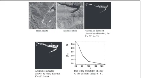
Figure 1Compressive target detection results under the AK ({αi}known) and AU ({αi}unknown) cases respectively as a function ofK.(a) Comparison of the worst-case empirical pFDR curves with the theoretical bounds when SNR is high.(b)Comparison of the results obtained by the proposed method using projection measurements usingΦdesigned according to (24),Φchosen at random, and the ones using downsampled measurements (DM) when the SNR is low.

case since they were derived under the assumption of{αi} being known. The experimental results are shown for both AK and AU cases to provide a comparison between the two scenarios. In both these cases, the worst-case empir-ical pFDR curves decay with the increase in the values of K. In the AK case, in particular, the worst-case empirical pFDR curve decays at the same rate as the upper bound. In this experiment, for a fixedαminanddmin, we choseK to satisfy (13c). The theory is somewhat conservative, and in practice the method works well even when the values of Kare below the bound in (13c).

In the experiment that follows, we letα∗_i ∼ U[ 10, 20], whereU denotes a uniform random variable,αi =

√ Kα∗_i and evaluate the performance of our detector for differ-ent values ofK that are not necessarily chosen to satisfy (13c). In addition, we also compare the performance of our detection method to that of a MAP based target detec-tor operating on downsampled versions of our simulated spectral input image. The reason behind such a compar-ison is to show what kinds of measurements yield better results given a fixed number of detectors.

For an input spectrumg∈RN, we letg∈RKdenote its downsampled approximation. Specifically, thejth element ofgiis"r=1g(j−1)r+wherer= N/K. Let us consider making observations of the form

y_i=gi

c +ni∈R

K ₍₂₃₎

whereg_i= αif∗i +biis theK-dimensional downsampled version off∗_i +biforK ≤N,ni ∼N(0,σ2I)forσ2= 5 andc is a constant that is chosen to preserve the mean signal-to-noise ratio corresponding to the downsampled and projection measurements. The MAP-based detec-tor operating on the downsampled data returns a label

DMAP_i for every observed spectrum which is determined according to

DMAP_i = arg min

∈{1,...,m},f()_∈D

y_i−αif() T

G−1

×y_i−αif() − logp()

where G = Σb+σ2I andΣb is the covariance matrix obtained from the downsampled versions of the back-ground training data andf()is the downsampled version off() ∈D. The algorithm declares that target spectrum

f(j)_{∈Dis present in theith location ifD}MAP

distance-preserving. This may worsen the performance as illustrated in Figure 1b.

Anomaly detection

In this section, we evaluate the performance of our anomaly detection method on (a) a simulated dataset and provide a comparison of the results obtained using the proposed projection measurements and the ones obtained using downsampled measurements, and (b) real AVIRIS (Airborne Visible InfraRed Imaging Spectrometer) dataset.

Experiments on simulated data

We simulate a spectral image f∗ composed of 8100 spectra, where each of them is either drawn from a dic-tionary D = {f(1),· · ·,f(5)} consisting of five labeled spectra from the HyMap data that correspond to a nat-ural landscape (trees, grass and lakes) or is anomalous. The anomalous spectrum is extracted from unlabeled AVIRIS data, and the minimum distance between the anomalous spectrumf(a) and any of the spectra inDis dmin = minf∈Df −f(a) = 0.5308. The simulated data

has 625 locations that contain the anomalous spectrum. Our goal is to find the spatial locations that contain the anomalous AVIRIS spectrum given noisy measurements of the formzi =Φ

αif∗i +bi

+wiwherebi∼(μb,Σb), Φ is designed according to (24), wi ∼ N(0,σ2I) and

f∗_i ∈ DunderH0i. As discussed in Section “Anomalous signal detection”,f∗_i is anomalous underH1i, and our goal is to control the FDR below a user-specified false discov-ery levelδ. We simulate{αi} =

√

Kα∗_i whereα_i∗∼U[ 2, 3]. In this experiment we assume the availability of back-ground training data to estimate the backback-ground statistics and the sensor noise varianceσ2. Given the knowledge of the background statistics, we perform the whitening transformation discussed in Section “Whitening compres-sive observations” and evaluate the detection performance on the preprocessed observations given by (2).

For a fixedτ = 0.1 and = 0.1, we evaluate the per-formance of the detector as the number of measurements K increases under the AK and AU cases respectively, by comparing the pseudo-ROC (receiver operating charac-teristic) curves obtained by plotting the empirical FDR against 1−FNR, where FNR is the false nondiscovery rate. Note that 1−FNR is the expected ratio of the number of null hypotheses that are correctly rejected to the number of declared null hypotheses. The empirical FDR and FNR are computed according to

FDR=

"M i=1ILGT

i =0

_I{p

i≤pt}

"M

i=1I{pi≤pt}

and

FNR=

"M i=1ILGT

i =1

_I{pi>p

t}

"M

i=1I{pi>pt}

wherept is thep-value threshold such that the BH pro-cedure rejects all null hypotheses for whichpi ≤ pt, and the ground truth labelLGT_i =0 if theith spectrum is not anomalous, and 1 otherwise. In this experiment, we con-sider three different values ofK approximately given by K ∈ {N/6,N/3,N/2} whereN = 106, and evaluate the performance of our detector for eachK. Furthermore, in our experiments with simulated data, we declare a spec-trum to be anomalous ifdi≥ηwhereηis a user-specified threshold anddi is defined in (16). We use thep-value upper bound in (20) in our experiments with real data where the ground truth is unknown.

We compare the performance of our method to a gener-alized likelihood ratio test (GLRT)-based procedure oper-ating on downsampled data, where we collect measure-ments of the form in (23) andf∗_i ∈DunderH0i. Observe thaty_i|H0i ∼ "f∈DP

f∗

i =f

N(αif,Σb+I), wheref refers to the downsampled version off ∈D. In this exper-iment we assume that each spectrum inDis equally likely underH0i fori = 1,. . .,M. The GLRT-based approach declares theith spectrum to be anomalous if

−logPy_i|H0i H1i

≷ H0i

η

0 0.1 0.3 0.5 0.7 0.9

FDR

1-FNR

K= 53

K= 26

K= 17

Pseudo-ROC plots, GLRT-based method operating on downsampled data using true values of

0 0.1 0.3 0.5 0.7 0.9 0.94

0.96 0.98 1

FDR

1-FNR

0.92

K= 53

K= 26

K= 17

Pseudo-ROC plots, Proposed method with chosen to be a random Gaussian projection matrix using true values of

0 0.1 0.3 0.5 0.7 0.9 0.92

0.94 0.96 0.98 1

FDR

1-FNR

K= 53

K= 26

K= 17

Pseudo-ROC plots, Proposed method where is designed according to (24) using true values of

0 0.1 0.3 0.5 0.7 0.9 0.94

0.96 0.98 1

FDR

1-FNR

K= 53; = 0.2

K= 26; = 0.3

K= 17; = 0.4

0.92

Pseudo-ROC plots, Proposed method where is designed according to (24) using ML estimates of

0 0.1 0.3 0.5 0.7 0.9 0.2

0.4 0.6 0.8 1

K= 53

K= 26

K= 17

pf

ROC plots, GLRT-based method operating on downsampled data using true values of

0 0.1 0.3 0.5 0.7 0.9 0.2

0.4 0.6 0.8 1

K= 53

K= 26

K= 17

pf

pd

ROC plots, Proposed method with chosen to be a random Gaussian pro-jection matrix using true values of

0 0.1 0.3 0.5 0.7 0.9 0. 2

0. 4 0. 6 0. 8 1

K= 53

K= 26

K= 17

pf

ROC plots, Proposed method where is designed according to (24) using true values of

0 0.1 0.3 0.5 0.7 0.9 0.2

0.4 0.6 0.8 1

pf

pd

K= 53; ζ= 0.2

K= 26; ζ= 0.3

K= 17; ζ

ζ ζ ζ

= 0.4

ROC plots, Proposed method where is designed according to (24) using ML estimates of

0.94 0.96 0.98 1

pd

pd

a

_b

c

d

f

e

h

g

Figure 2Comparison of the performances of the proposed anomaly detector using a randomΦ, the proposed anomaly detector using the designedΦin (24) and the GLRT-based method operating on downsampled data for different values ofKwhenα∗_i ∈U[ 2, 3]and αi=α∗

i

√

in a finite collection, where as the downsampled mea-surements fail to preserve distances among vectors that are very similar to each other. Similarly, a random pro-jection matrix Φ is not necessarily distance-preserving post-whitening transformation, which leads to poor per-formance as illustrated in Figure 2b,f. Figure 2d,h shows the pseudo-ROC plots and the conventional ROC plots obtained using our method when{αi}are unknown, and are estimated from the measurements. Note that the value ofζ decreases asK increases since the estimation accu-racy of{αi}increases with increase inK. These plots show that the performance improves as we collect more obser-vations, and that, as expected, the performance under the AK case is better than the performance under the AU case.

Experiments on real AVIRIS data

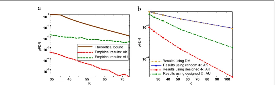
To test the performance of our anomaly detector on a real dataset, we consider the unlabeled AVIRIS Jasper Ridge datasetg ∈ R614×512×197, which is publicly avail-able from the NASA AVIRIS website, http://aviris.jpl.nasa. gov/html/aviris.freedata.html. We split this data spatially to form equisized training and validation datasets,gtand

gv_{respectively, each of which is of size 128×128×197.} Figure 3a,b show images of the AVIRIS training and val-idation data summed through the spectral coordinates. The training data are comprised of a rocky terrain with a small patch of trees. The validation data seems to be made of a similar rocky terrain, but also contain an anomalous

lake-like structure. The goal is to evaluate the perfor-mance of the detector in detecting the anomalous region in the validation data for different values ofK. We clus-ter the spectral targets in the normalized training data to eight different clusters using the K-means clustering algorithm and form a dictionary D comprising of the cluster centroids. Given the dictionary and the validation data, we find the ground truth by labeling theith valida-tion spectrum as anomalous if minf∈Df − g

v i gv i

> τ. Since the statistics of the possible background contamina-tion in the data could not be learned in this experiment because of the lack of labeled training data, the dictionary might be background contaminated as well. The param-eterτ encapsulates this uncertainty in our knowledge of the dictionary. In this experiment, we setτ =0.2.

We generate measurements of the formy_i=√Kgv_i +ni fori=1,. . ., 128×128, whereni∼N(0,I). The

√ K fac-tor indicates that the observed signal strength increases withK. For a fixed FDR control value of 0.01, Figure 3c,d shows the results obtained forK ≈ N/5 andK ≈ N/2, respectively. Figure 3e shows how the probability of error decays as a function of the number of measurements K. The results presented here are obtained by averaging over 1,000 different noise and sensing matrix realiza-tions. From these results, we can see that the number of detected anomalies increases withK and the number of misclassifications decrease withK.

Trainingdata Validationdata Anomalies detected (shown by white dots) for K≈N/ 5 = 39.

Anomalies detected (shown by white dots) for K≈N/2 = 99.

20 60 100 140 180 0.01

0.02 0.03 0.04 0.05 0.06

K

p

Plot of the probability of error p_{e for different values of K.}

a

b

c

d

e

Conclusion

This work presents computationally efficient approaches for detecting known targets and anomalies of different strengths from projection measurements without per-forming a complete reconstruction of the underlying sig-nals, and offers theoretical bounds on the worst-case tar-get detector performance. This article treats each signal as independent of its spatial or temporal neighbors. This assumption is reasonable in many contexts, especially when the spatial or temporal resolution is low relative to the spatial homogeneity of the environment or the pace with which a scene changes. However, emerging technolo-gies in computational optical systems continue to improve the resolution of spectral imagers. In our future work we will build upon the methods that we have discussed here to exploit the spatial or temporal correlations in the data.

Appendix 1: Proof of Theorem 1

Using linear algebra and matrix theory, it is possible to show that ifB=I−AΣbATis positive definite, then

Φ=σB−1/2_{A (24)}

satisfies (3).c _{In particular, we can substitute (24) in (3)} to verify that the proposed construction ofΦsatisfies (3). Observe thatC_Φ = ΦΣbΦT+σ2_I−1/2_{can be written} in terms of (24) as follows:

CΦ = σB−12A

#

Σb σB−

1 2A

#T +σ2_I

−1 2

=

σ2_B−1/2_AΣ bAT

B−12

T +σ2_I

−1 2

=

σ2_B−1_2(I−B)B−1₂ T_+σ2_I −1

2

=σ2_B−1−12 =σ−1B1_{2 (25)}

where the third-to-last equation follows from the defini-tion ofBand (25) follows from the fact thatBis symmetric and positive definite. IfBis positive definite, thenB−1is positive definite as well and can be decomposed asB−1=

B−1/2T_B−1/2_{, where the matrix square root B}−1/2 _is symmetric and positive definite. By substituting (25) and (24) in (3), we have CΦΦ = σ−1B1/2σB−1/2A = A. A sufficient condition for Bto be positive definite can be derived as follows.

To ensure positive definiteness ofB, we must have

xT_Bx=xT_x−xT_AΣ

bAT x>0 (26)

for any nonzero x ∈ RK. Note that sinceΣb is positive semidefinite,xTAΣbATx≥0. However, the right hand side of (26) is> 0 only if the spectral norm ofAΣbAT is

< 1, sincexTAΣbATx≤ x2· AΣbAT. The norm ofAΣbATis in turn bounded above by

AΣbAT ≤ AΣbAT = A2Σb = A2λmax

since A = AT and Σb = λmax, whereλmax is the largest eigenvalue of Σb. To ensureAΣbAT < 1, A2_λ

max has to be < 1, which leads to the result of Theorem 1.

Appendix 2: Proof of Theorem 2

The proof of Theorem 2 adapts the proof techniques from [48] to nonidentical independent hypothesis tests. We begin by expanding the pFDR definition in (8) as follows:

pFDR(j)(Γ)= M

k=1 E

V(Γ) R(Γ)

R(Γ)=k

×P(R(Γ)=k|R(Γ) >0).

Observe thatR(Γ)=kimplies that there exists some sub-setSk= {u1,. . .,uk} ⊆ {1,. . .,M}of sizeksuch thatyu ∈

Γu(j)for=1,. . .,kandyi ∈Γ( j)

i for alli ∈Sk. To simplify the notation, letΛSk =

$ u∈SkΓ

j

u×$/∈SkΓ (j)

, whereΓ(j)

is the complement ofΓ(j), denote the significance region that corresponds to set Sk, and T = (y1,. . .,yM) be a set of test statistics corresponding to each hypothesis test. Considering all such subsets we have

pFDR(j)(Γ)= M

k=1

Sk

E

V(Γ) k

T∈ΛSk

×PT∈ΛSkR(Γ) >0

. (27)

By plugging in the definition ofV({Γi})from (9), we have

E%V(Γ)|T∈ΛS_k&=E

' _M

i=1

I

y_i∈Γ(j)

i _I

H(j)

i =0

T∈ΛSk ( ≡ k =1 E I

H(j)

u=0 _y u = k =1

PH(j)

u=0yu∈Γ( j) u

(28)

for allu∈Sksince the tests are independent of each other givenA. The posterior probabilityP

H(j)

i =0yi∈Γ( j)

i for the ithhypothesis test can be expanded using Bayes’ rule as

PH(j)

0i yi∈Γ( j)

i =

Py_i∈Γ(j)

i |H0i P

H(j)

0i

Py(j)

i ∈Γ (j) i

≡ P

f_i =f(j)_f∗

i =f(j) P

f∗_i =f(j)

Pf_i =f(j) ,