R E S E A R C H
Open Access
Integrating artificial neural network and classical
methods for unsupervised classification of optical
remote sensing data
Ahmed AK Tahir
Abstract
A novel system named unsupervised multiple classifier system (UMCS) for unsupervised classification of optical remote sensing data is presented. The system is based on integrating two or more individual classifiers. A new dynamic selection-based method is developed for integrating the decisions of the individual classifiers. It is based on competition distance arranged in a table named class-distance map (CDM) associated to each individual classifier. These maps are derived from the class-to-class-distance measures which represent the distances between each class and the remaining classes for each individual classifier. Three individual classifiers are used for the development of the system, K-means and K-medians clustering of the classical approach and Kohonen network of the artificial neural network approach. The system is applied to ETM + images of an area North to Mosul dam in northern part of Iraq. To show the significance of increasing the number of individual classifiers, the application covered three modes, UMCS@, UMCS#, and UMCS*. In UMCS@, K-means and Kohonen are used as individual classifiers. In UMCS#, K-medians and Kohonen are used as individual classifiers. In UMCS*, K-means, K-medians and Kohonen are used as individual classifiers. The performance of the system for the three modes is evaluated by comparing the outputs of individual classifiers to the outputs of UMCSs using test data extracted by visual interpretation of color composite images. The evaluation has shown that the performance of the system with all three modes outrages the performance of the individual classifiers. However, the improvement in the class and average accuracy for UMCS* was significant compared to the improvements made by UMCS@, and UMCS#. For UMCS*, the accuracy of all classes were improved over the accuracy achieved by each of the individual classifiers and the average improvements reached (4.27, 3.70, and 6.41%) over the average accuracy achieved by K-means, K-medians and Kohonen respectively. These improvements correspond to areas of 3.37, 2.92 and 5.1 km2 respectively. While the average improvements achieved by UMCS@ and UMCS#, respectively, compared to their individual classifiers were (0.77 and 2.79%) and (0.829 and 2.92%) which correspond to (0.61 and 2.2 km2) and (0.65 and 2.3 km2) respectively.
Introduction
Unsupervised classification of remotely sensed data is a technique of classifying image pixels into classes based on statistics without pre-defined training data. This means that the technique is of potential importance when train-ing data representtrain-ing the available classes is not available. Unsupervised classification is also important for providing a preliminary overview of image classes and more often it is used in the hybrid approach of image classification [1,2].
Several methods of unsupervised classification using clas-sical or neural network approaches have been developed and used consistently in the field of remote sensing. The most commonly used of the classical approach is K-means clustering algorithm [3] while Kohonen network is the most commonly used one of the artificial neural network approach [4]. So far many research works have conducted to improve the accuracy of the unsupervised classifiers. Examples of these works are the use of Kohonen classifier as a pre-stage to improve the results of clustering algorithms such as agglomerative hierarchical clustering, K-means and threshold-based clustering algorithms [5-7]. Correspondence:[email protected]
Department of Computer Science, Faculty of Science, Duhok University, Duhok, Kurdistan Region, Iraq
In those works one algorithm was used as a pre-stage to improve the classification results of another algorithm. That is, the final decision is made according to only one classifier’s decision. Methods involving a simultaneous use of more than one classifier in the so-called multiple classi-fier system (MCS) which is very common in the approach of supervised classification have not been conducted in the unsupervised classification of optical remote sensing data. See for example [8-10] for some of the MCS schemes form supervised classification of remote sensing data. The idea of MCS is based on performing more than two classi-fiers and integrating their decisions according to some prior or posterior knowledge concerning the output classes to reach the final decision. Prior knowledge is esti-mated from training data concerning the output classes while posterior knowledge, in general, represents the out-puts of the individual classifiers. The operation of integra-tion is done in one of two strategies, either by combining the outputs of the individual classifiers or by selecting one of the individual classifiers outputs. Many methods of in-tegration have been developed for the implementation of MCS in the supervised approach of classification. Exam-ples of combined-based methods of integration are the majority voting rule, which assigns the label scored by ma-jority of the classifiers to the test sample [9] and Belief function, which is knowledge-based method. It is based on the probability estimation provided by the confusion matrix derived from training data set [11]. Examples of the dynamic classifier selection-based method of integra-tion are classifier rank (CR) approach, which takes the de-cision of the classifier that correctly classifies most of the training samples neighboring the test sample [12] and the local ranking (LR) which is based on ranking the individ-ual classifiers for each class according to the mapping accuracy (MA) of the classes [8].
In this article, an integrated system of unsupervised classification named unsupervised multiple classifier sys-tem (UMCS) is developed using individual classifiers from two different approaches, traditional (classical) and artificial neural network. The system is based on new in-tegration method of the dynamic classifier selection-based type. This method is selection-based on class-distance maps (CDM) for the individual classifiers as the measure upon which the final decision is selected. The CDM of each individual classifier is generated from the measure of Eu-clidean distances between each class and the remaining classes of that individual classifier, named here as the class-to-class distance measurement (CCDM).
The remaining parts of the article are organized as fol-lows: In the following section, the proposed system is described and detailed explanations of its major modules are given. In section“Results”, the results of applying the system to ETM + images are shown and discussed. In section “Posterior interpretation of output classes”,
posterior interpretation of the classification outputs is done. In section “Individuals and multiple classifiers comparison”, comparisons between the output results are made. In section“Evaluation of system performance”, the performance of the system is evaluated and finally some concluding remarks are given in the last section.
(UMCS); the proposed system
In this article, the proposed system of classification is called UMCS to be differentiated from the multiple clas-sifier system (MCS) which is common in supervised classification. It is designed to host three individual un-supervised classifiers and can be adapted to any number on individual classifiers. The scheme of the system for three individual classifiers is shown in Figure 1. Each of the three classifiers, K-means, K-medians and Kohonen is implemented using multi-spectral images yielding three output images. These three output images are then entered to a color unification algorithm (CUA) in order to achieve class-to-class correspondence in the three output images. Finally, the three output images of the (CUA) are integrated using CDM generated from the Euclidean dis-tance measurements between each class and the remaining classes within the classifier, named as (CCDM). The algorithms of color unification and classifier integra-tion method are given in the following secintegra-tions.
CUA
In most cases the order of classes resulting from differ-ent approaches of unsupervised classification are affected by the way of performing the operation of clus-tering and the order of data presented to the process of clustering. For instance, in the Kohonen network, the training phase usually starts by giving the initial weights
which control the order of the outcome classes. There-fore in order to implement the proposed system, the corresponding classes in the individual classifiers must have the same order. To achieve this step, an algorithm named CUA is developed. The aim of this algorithm is to reorder the classes an all classifiers in order to assign same color to the three nearest classes of the three clas-sifiers. This is done by fixing the order of classes in one classifier as a reference and reordering the classes of the other two classifiers. This algorithm requires the deter-mination of the Euclidean distance between the center of each class in the referenced classifier and the centers of all classes in each of the other two classifiers. The nearest two classes each from one classifier are given the same order (color) of the current class in the reference classifier. Then the operation is repeated until the order-ing of all classes in the three classifiers is reached. The algorithm does not require re-calculation of the class cen-ters since these cencen-ters are calculated during the imple-mentation of the classifiers. In K-means and K-medians classifiers, the last mean vectors and median vectors upon which the classifier have reached the convergence state represent the centers of the classes. In Kohonen classifier, the weight vectors to the output neurons are taken to be the centers of the classes. The procedures of the algorithm are:
1- Read the centers of the classes for the three classifiers and set the class number i = 0. 2- Increase class number i = i + 1.
3- Calculate the Euclidean distance between the mean vector of Cifrom the reference classifier and the
mean vectors of all output classes in the other two classifiers.
Dim ¼ jjCiPmjjfor all m ¼ i; ; ;k
Din ¼ jjCiQnjjfor all n ¼ i; ; ;k
Where;
Dimis the Euclidean distance between class Cifrom
the reference classifier and class Pmfrom the second
classifier.
Dinis the Euclidean distance between class Cifrom
the reference classifier and class Qnfrom the third
classifier.
||.|| represents the norm operator. 4- Exchange class order.
Exchange the class order of the second classifier: if D ij<Dim for all m¼i; ; ;k and j≠m Temp = Pj
Pj= Pi
Pi= Temp
Exchange the class order of the third classifier: if Dð il<Din Þ for all n¼i; ; ;k and l≠n
Temp = Ql
Ql= Qi
Qi= Temp
5- Check the convergence of the algorithm. if (i < k)
Go to step 2 else
Go to step 6 6- Stop.
Integration method by CCDM
As it was mentioned in the introduction, several meth-ods of integrating the outputs of different classifiers are available. These methods were designed for MCS of the supervised type and they require a priori knowledge which most often can be estimated from the training data. For UMCS, the training data are not available and therefore this a priori knowledge cannot be obtained. The method of majority voting may be the only one which can be used to integrate the outputs of unsuper-vised classifiers since it only requires the final decisions of the three classifiers. However, this rule is influenced by the degree of correlation among the errors made by individual classifiers. When these errors are correlated (all classifiers produce incorrect but similar outputs) it leads to incorrect decision and when these errors are uncorrelated (each classifier produces a unique output) it leads to failure, [9].
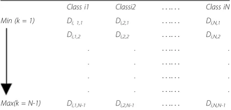
In this article, a new method of integration is intro-duced. It is categorized as a selection-based approach and does not need prior knowledge. It requires a poster-ior knowledge which can be obtained from the outputs of the three classifiers. This posterior knowledge is the within classifier CCDM which is the measure of Euclid-ean distance between each class and all of the remaining classes within each individual classifier. This CCDM is then used to generate a table having N columns and N-1 rows, where N is the number of classes. The elements under each column represent the distances, stored in ascending way, from the class of that column to all of the remaining classes. For each individual classifier one CDM is generated.
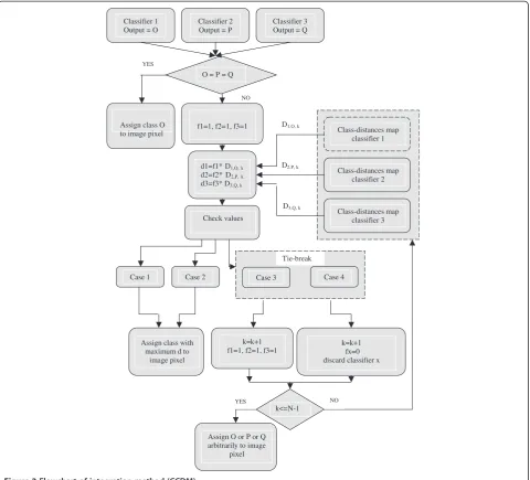
The procedures of implementing the algorithm are given below for UMCS made from three classifiers. It consists of two parts. In the first part, the CDM is gener-ated. In the second part, the process of selecting the final decision is performed. The algorithm can easily be adapted to any number of classifiers. The flowchart of the algorithm is given in Figure 2.
Generation of CDM
CCDMij¼
X
jjCiCjjj ð1Þ
Where;
i = 1,,,,N, j = 1,,,,N, i≠j and N is the number of classes in each classifier.
||.|| represents the norm operator.
Ciis the mean vector of ithclass and Cjis the mean
vector of jthclass, both from the same classifier. For N classes there will be N-1 distances associated with each class.
2- Generate CDM by sorting the values of CCDM in an ascending way to be used for competition between the individual classifiers. Let these competition distances be represented as Di,j,k, where;
i is a subscript refers to the individual classifier, i = 1,,,M and M is the total number of individual classifiers involved in the UMCS.
j refers to the current class, j = 1,,,N and N is the number of classes which is the same for all individual classifiers.
k refers to the position of the distances after being sorted in an ascending way. That is, the minimum of all will be at the top of column with position k = 1 and the maximum of all will be at the bottom of column with position k = N-1. During the process of decision selection, these distances at position k = 1 will be compared and at tie cases the distances at the next position k = 2 will be compared and so on until Classifier 1
Output = O
Classifier 2 Output = P
Classifier 3 Output = Q
YES
O = P = Q
NO
Assign class O to image pixel
f1=1, f2=1, f3=1
d1=f1* D1,O, k d2=f2* D2,P, k d3=f3* D3,Q, k
D1,O, k
D2,P, k
Class-distances map classifier 1
Class-distances map classifier 2
Check values
D3,Q, k
Class-distances map classifier 3
Tie-break Case 1 Case 2 Case 3 Case 4
Assign class with maximum d to
image pixel
k=k+1 f1=1, f2=1, f3=1
k=k+1 fx=0 discard classifier x
YES NO
k<=N-1
Assign O or P or Q arbitrarily to image
pixel
tie break is achieved. If the tie case continued to appear until the last position, which is a rarely occurred case, then it is broken by assigning the class produced by one of the individual classifier arbitrarily. This way of comparison makes the algorithm effective for tie cases as there will almost a zero chance for the occurrence of tie while
comparing all the competitive distances. Table1
shows a model of CDM for classifier i. In this table, each column holds the competition distances associated to each class, starting from class 1 to class N. UMCS of three individual classifiers requires three of these CDM and during the operation of decision selection there will be a competition between these distances in three column each of one CDM.
3- Read the three output images produced by the three individual classifiers pixel by pixel. The values of these pixels represent the class numbers produced by the three classifiers. Let these class numbers are: O, P and Q. Then perform the following statements: if (O = P and O = Q) then
Assign class O to the pixel of the final output image Else
Perform the operation of integrating the decisions made by the three classifiers.
Performing the process of final decision selection
1- Set record number k to a value of one (the position of the first distance in each of the columns under the output classes) and set three flags (f1, f2, f3) each to a value of one.
2- Read the distances associated to these classes at position k (D1,O,k, D2,P,k, D3,Q,k).
3- Compute competitive distances (d1, d2, d3) as follows:
d1 = f1* D1,O,k
d2 = f2* D2,P,k
d3 = f3* D3,Q,k
4- Check the values of these competitive distances to perform one of the following cases for final decision:
Case 1: If these competitive distances are alternatively different, then assign the class with maximum competitive distance to the pixel of the final output image. Case 2: If any two of these competitive
distances have the same value and this value is lower than the competitive distance of the other class, then assign the other class to the pixel of the final output image.
Case 3 (Tie-Break): If the competitive distances for the three classes are all the same, then increase k by one and go to step 2 to read the next associated distances. If the tie case
remained unbroken, then assign one of the classes arbitrarily to the pixel of the final output image.
Case 4 (Tie-Break): If the competitive distances of any two classes have same value and this value is greater than the competitive distance of the other class, then discard the other class from competition by resetting its flag (f ) to zero and increase k by one then go to step 2. Here, the competition will remain between two output classes as far as the tie is not broken and if k value reached the last record at a position number equals (m - 1) where m is the total number of classes without achieving tie-break, then assign one of the classes arbitrarily to the pixel of the final output image, otherwise assign the class with maximum competitive distance to the pixel of the final output image.
Results
The system is applied to ETM + image of an area north to Mosul dam in the northern part of Iraq. The image size is 296 × 296 square pixels which is equivalent to an area of 78.85 km2. Standard Kohonen network with R = 0 was used (the weights of only the winner neuron are updated). The number of neurons in the input layer was chosen to be 6 which is the number of the available bands Table 1 A model of CDM for classifier i
Class i1 Classi2 . . .. . . Class iN
Min (k = 1) Di, 1,1 Di,2,1 . . .. . . Di,N,1
Di,1,2 Di,2,2 . . .. . . Di,N,2
. . . . .. . . .
. . . . .. . . .
. . . . .. . . .
. . . . .. . . .
of ETM + (band1, band2, band3, band4, band5 and band7). The number of neurons in the output layer was chosen to be 8 which are the same as the output classes in K-means and K-medians. However in practice, train-ing Kohonen network usually needs wise determination of the learning rate and the number of cycles. In this article, different values of learning rate and cycle num-bers were tried. Consistent results were reached by using initial learning rate of 0.7 with a decrement of (0.7/500) at each next cycle where the number of cycles is taken to be 500. Kohonen neural network with this structure is supposed to be closest to K-means than any of the other structures of Kohonen neural network. K-medians clustering is a variation of K-means, how-ever mathematically medians are calculated instead of means, [13].
The selection of standard Kohonen neural network and the K-medians as being closely related to K-means cluster-ing was done in order to show that, to what extend these classifiers can produce different results and to what ex-tend the application of UMCS can be appreciable when individual classifiers of divers differences are chosen.
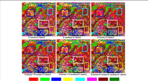
The system is applied in three modes using different number and combinations of individual classifiers in order to show the influence of increasing the number of individual classifiers on the system accuracy. In the first mode (UMCS@), K-means and Kohonen were used as two individual classifiers. In the second mode (UMCS#), K-medians and Kohonen were used as two
individual classifiers. In the third mode (UMCS*), K-means, K-means and Kohonen were used as three in-dividual classifiers. Figure 3, shows the classification results of K-means, K-means, Kohonen and the three multiple classifiers UMCS@, UMCS#, and UMCS*. In unsupervised classification usually the number of classes is chosen either arbitrarily or according to the available knowledge of the study area. Here, this num-ber was chosen to be 8 after visual inspection of the color composite images made from different combina-tions of the available bands.
To show as to what extend the individual classifiers in each MCS agreed or disagreed in their decisions are given in Table 2. In this table, the percentages of pixels and their equivalent areas for which all the individual classifiers produced the same and different decisions for the three MCS (UMCS@, UMCS#, and UMCS*) are shown. According to this table the number of pixels for which the individual classifiers have given different results in the case of UMCS* is greater than those in UMCS@ and UMCS#. This is an expected result given the fact that increasing the number of individual classi-fiers will makes more chances of these classiclassi-fiers first to give different results and second to produce uncorre-lated errors, [14].
Posterior interpretation of output classes
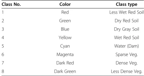
In unsupervised classification the cover types that repre-sent the output classes must be identified after the
classification. Here, this interpretation was done by com-paring the results of the individual classifiers and the multiple classifiers visually to the color composite images of the available bands. Two color composite images were generated using the combinations (band4, band3, band2 as RGB) and (band7, band4, band1 as RGB), Figure 4. First, the interpretation of these color composite images was implemented by comparing the colors in these two color composite images to the spec-tral properties of the cover types. This is one of the most commonly used methods for remote sensing data inter-pretation, [4]. Table 3 shows the identities of the output classes after interpretation.
Individuals and multiple classifiers comparison To visualize the differences between the outputs of the six classifiers, five areas were localized in rectangles of different colors. These differences can be illustrated for the area in black rectangle. Figure 5 is the zoomed image of the black rectangles for the six classifiers. In the prod-uct of K-means the area of this rectangle is dominated by blue and yellow colors, which correspond to (Dry
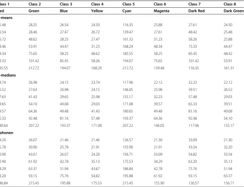
Gray Soil) and (Wet Red Soil) cover types respectively. However, the area of blue color within this rectangle for K-means and K-medians are almost the same. In the product of Kohonen, two more colors appeared in this rectangle, the green and some patches of red colors which correspond to (Dry Red Soil) and (Less Wet Red Soil). These variations in the colors within this rectangle indicate that the three individual classifiers can produce different results for the same area. Looking at this rect-angle in the UMCS products shows that these colors have been distributed differently for the three UMCS products. For instance in UMCS@ and UMCS* pro-ducts, the colors and their distributions are almost the same as in K-means. This indicates that the competition between the blue and yellow colors of K-means product on one side and the green, magenta and red colors of the K-medians and Kohonen products on the other side was in favor of K-means classifier. This can be checked by looking at the CDM of the three individual classifiers, Table 4. This table shows that the competitive distance of blue in K-means is higher than the competitive Table 2 Image size percentages and their equivalent
areas for which the individual classifier in each of UMCSs produce the same and different decisions
UMCS Same decision Different decision
UMCS@ percentage 69.73% 30.27%
Equivalent area 54.98 km2 23.87 km2
UMCS# percentage 71.60% 28.40%
Equivalent area 56.46 km2 22.39 km2
UMCS* percentage 60.29% 39.71%
Equivalent area 47.54 km2 31.31 km2
Figure 4Two color composite images band4, band3, and band2 as RGB and band7, band4, and band1as RGB. Table 3 Identities of output classes
Class No. Color Class type
1 Red Less Wet Red Soil
2 Green Dry Red Soil
3 Blue Dry Gray Soil
4 Yellow Wet Red Soil
5 Cyan Water (Dam)
6 Magenta Sparse Veg.
7 Dark Red Dense Veg.
distance of green color in Kohonen, therefore blue color will be the winner and will appear in the output of the MCS. On the other hand, the competition distance of
yellow colors of the K-means map is greater than the competitive distance of magenta and red colors in the maps of K-medians and Kohonen therefore, in the Figure 5Zoomed details within black rectangles for the individual and multiple classifiers.
Table 4 CDM
Class 1 Class 2 Class 3 Class 4 Class 5 Class 6 Class 7 Class 8
Red Green Blue Yellow Cyan Magenta Dark Red Dark Green
K-means
25.48 28.25 26.54 24.50 116.35 25.88 27.61 24.50
26.54 28.46 27.47 26.72 139.47 27.61 48.42 25.48
26.72 48.62 28.25 27.47 161.32 31.23 58.26 25.88
28.46 53.91 44.47 31.23 168.29 48.34 73.33 44.47
48.34 75.65 58.25 48.62 185.55 58.25 85.45 48.42
73.33 101.42 85.45 58.26 194.07 75.65 101.42 53.91
185.55 212.72 194.07 168.29 212.72 139.48 116.35 161.31
K-medians
23.74 26.98 24.15 23.74 117.96 22.12 32.23 22.12
26.52 27.63 26.98 24.15 146.05 25.98 39.51 26.52
27.63 41.43 29.65 25.98 155.17 32.23 57.48 29.03
29.65 54.10 49.08 29.03 171.08 39.57 65.33 39.51
39.57 64.36 49.48 41.43 180.65 49.48 81.16 49.08
65.33 92.48 81.16 57.48 193.37 64.36 92.48 54.10
180.64 207.22 193.37 171.08 207.22 146.05 117.96 155.17
Kohonen
24.20 26.07 21.46 21.46 126.57 21.30 33.09 21.30
25.78 30.90 25.78 21.91 155.90 21.91 33.54 32.20
30.90 43.67 26.07 24.20 156.71 33.09 54.82 33.54
32.90 61.92 42.78 35.13 175.53 34.29 63.20 35.13
34.29 63.37 51.94 43.67 186.84 42.78 75.76 51.94
63.20 93.15 75.76 54.82 195.88 61.92 93.15 63.37
186.84 215.45 195.88 175.53 215.45 155.90 126.57 156.71
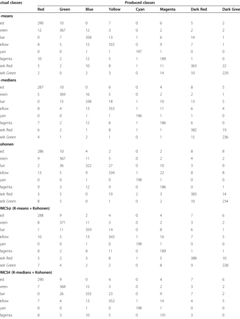
Table 5 Confusion matrices of the individual and multiple classifiers
Actual classes Produced classes
Red Green Blue Yellow Cyan Magenta Dark Red Dark Green
K-means
Red 290 10 0 7 0 6 5 2
Green 12 367 12 3 0 2 2 2
Blue 0 7 358 13 1 6 14 1
Yellow 8 5 15 355 0 9 7 1
Cyan 0 0 1 1 197 1 0 0
Magenta 10 2 12 5 1 189 1 0
Dark Red 3 2 10 8 1 11 363 22
Dark Green 2 0 2 3 0 14 10 229
K-medians
Red 287 10 0 6 0 4 8 5
Green 5 369 16 5 0 2 2 1
Blue 0 15 338 18 1 10 13 5
Yellow 8 4 13 353 1 11 6 4
Cyan 0 0 1 1 196 1 1 0
Magenta 7 2 12 6 1 186 6 0
Dark Red 6 2 1 8 1 1 382 19
Dark Green 4 1 2 1 0 1 15 236
Kohonen
Red 286 10 4 2 0 2 8 8
Green 9 367 11 5 0 2 4 2
Blue 2 36 322 27 0 10 3 0
Yellow 13 5 9 334 1 22 8 8
Cyan 0 0 1 0 198 1 0 0
Magenta 9 3 12 9 0 186 0 1
Dark Red 3 5 0 10 2 3 383 14
Dark Green 8 5 0 1 0 2 10 234
UMCS@ (K-means + Kohonen)
Red 288 9 2 4 0 4 7 6
Green 8 371 11 3 0 2 3 2
Blue 1 11 359 14 0 8 6 1
Yellow 10 5 13 343 1 16 7 5
Cyan 0 0 1 0 198 1 0 0
Magenta 8 2 8 11 0 189 1 1
Dark Red 3 2 3 8 1 5 388 10
Dark Green 7 4 2 2 0 8 9 228
UMCS# (K-medians + Kohonen)
Red 290 9 0 4 0 4 7 6
Green 7 368 15 3 0 2 3 2
Blue 0 26 333 23 0 9 7 2
Yellow 7 4 13 352 1 14 4 5
Cyan 0 0 1 0 198 1 0 0
output of MCS UMCS* yellow color will be the winner. The same rule can be applied to areas within the other rectangles with the aid of CDM of the individual classifiers.
Evaluation of system performance
The performance of the system was evaluated by select-ing test data from the two color composite images repre-senting the eight classes. The locations of these test data samples were shown as rectangles in the color compos-ite of (Band4, band3, band2 as RGB) of Figure 4. For each class the rectangle is shown in the same color of that class. The numbers of the selected pixels for the classes 1 to 8 respectively were 320, 400, 400, 400, 200, 220, 420 and 260). This data is then entered to each of the individual classifier (K-means, K-medians and Kohonen) as well as to each of the multiple classifiers (UMCS@, UMCS# and UMCS*).
The MA was measured since this measurement takes into account the pixels that are falsely classified. The
confusion matrices of the six classifiers are given in Table 5. In this table, the diagonal elements represent the number of pixels that are correctly classified (Pcorr), the off-diagonal elements in the row of the class repre-sent the number of pixels that are incorrectly classified to other classes, known as omission error (Pom)and the off-diagonal elements in the column of the class repre-sent pixels that are falsely classified to the current class, known as commission error (Pcom). The MA of the eight classes for each classifier is calculated using the follow-ing equation:
MA¼P Pcorr
corrþPomþPcom ð2Þ
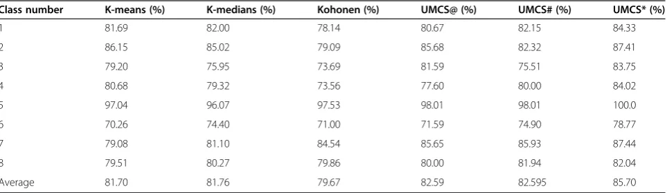
Table 6 shows these mapping accuracies for the six classifiers. It can be seen that the MA of all classes are improved by UMCS*, while the MA for some classes were improved and for others were decreased by UMCS@ and UMCS# classifiers. Table 7 shows the
Table 6 The accuracy mapping of the individual and multiple classifiers
Class number K-means (%) K-medians (%) Kohonen (%) UMCS@ (%) UMCS# (%) UMCS* (%)
1 81.69 82.00 78.14 80.67 82.15 84.33
2 86.15 85.02 79.09 85.68 82.32 87.41
3 79.20 75.95 73.69 81.59 75.51 83.75
4 80.68 79.32 73.56 77.60 80.00 84.02
5 97.04 96.07 97.53 98.01 98.01 100.0
6 70.26 74.40 71.00 71.59 74.90 78.77
7 79.08 81.10 84.54 85.65 85.93 87.44
8 79.51 80.27 79.86 80.00 81.94 82.04
Average 81.70 81.76 79.67 82.59 82.595 85.70
UMCS@ is multiple of K-means + K-medians. UMCS# is multiple of K-medians + Kohonen. UMCS* is multiple of K-means + K-medians + Kohonen.
Table 5 Confusion matrices of the individual and multiple classifiers(Continued)
Dark Red 5 3 1 4 1 2 391 13
Dark Green 6 2 1 1 0 3 11 236
UMCS* (K-means + K-medians + Kohonen)
Red 296 8 0 2 0 2 5 7
Green 7 375 10 3 0 2 1 2
Blue 0 9 366 12 0 5 6 2
Yellow 7 3 12 363 0 7 5 3
Cyan 0 0 0 0 200 0 0 0
Magenta 6 3 11 5 0 193 1 1
Dark Red 4 2 2 8 0 5 390 9
Dark Green 7 4 2 2 0 4 8 233
improvements in the class and average MA made by each of the multiple classifiers over their belonging indi-vidual classifiers. The best improvements were achieved by UMCS* over each of the individual classifiers. The amounts of these improvements are 4.27, 3.70 and 6.41% over each of K-means, K-medians and Kohonen classifiers respectively. These improvements are equiva-lent to areas of 3.37, 2.92 and 5.1 km2. Whereas the average improvements made by UMCS@ and UMCS#, over each of the individual classifiers were much less. For UMCS@ the improvement over K-means and Kohonen were 0.77 and 2.79% (equivalent to areas of 0.61 and 2.2 km2) and for UMCS# the improvement over K-medians
and Kohonen were 0.829 and 2.92% (equivalent to areas of 0.65 and 2.3 km2). However, for individual classes the maximum improvement achieved by UMCS* reached 8.51, 7.80 and 10.46% over each of K-means, K-medians and Kohonen classifiers respectively. While the improve-ments made by UMCS@ over K-means and Kohonen were 6.57 and 6.59% respectively and by UMCS# over K-medians and Kohonen were 4.83 and 6.44% respect-ively. These improvements indicate that when more classifiers are used in the multiple classifier system better improvement can be achieved. This concluded result has also been approved for the supervised mul-tiple classifier system, [14].
Table 7 Amount of improvements in the MA
Class number UMCS@-K-means (%) UMCS@-Kohonen (%)
Improvement of UMCS@ over each of K-means and Kohonen
1 −0.98 +2.53
2 −1.53 +6.59
3 +2.39 +7.90
4 −3.08 +3.04
5 +0.97 +0.48
6 +1.33 +0.59
7 +6.57 +1.11
8 +0.49 +0.14
Average +0.77 +2.79
Improvement of UMCS# over each of K-medians and Kohonen
1 +0.15 +4.01
2 −2.70 +3.23
3 −0.44 +1.82
4 +0.68 +6.44
5 +1.94 +0.48
6 +0.50 +3.90
7 +4.83 +1.39
8 +1.67 +2.08
Average +0.829 +2.92
Improvement of UMCS* over each of K-means, K-medians and Kohonen
Class number UMCS*-K-means (%) UMCS*-K-medians (%) UMCS*-Kohonen (%)
1 +2.64 +2.33 +6.19
2 +1.26 +2.39 +8.32
3 +4.55 +7.80 +10.06
4 +3.34 +4.70 +10.46
5 +2.96 +3.93 +2.47
6 +8.51 +4.37 +8.77
7 +8.36 +6.34 +2.90
8 +2.53 +1.77 +2.18
Average +4.27 +3.70 +6.41
Conclusions
Unsupervised classifiers (K-means, K-medians and Kohonen) representing two different approaches, clas-sical and artificial neural network, they were integrated in a MCS the application of the system to satellite images has shown that the three classifiers may produce different results despite of being considered as closely related. The CDM, which is generated from the CCDM, is shown to be effective measure for competition during the process of classifier output integration. The way of using the record of this map makes the chance of tie cases occurrence as less as possible. For the area used in this study no tie cases have occurred. The implementa-tion of the system does not need training data; however, the test data derived after classification are necessary only for the evaluation of the system performance. The application of the system using three individual classi-fiers achieved better performance than its application with only two individual classifiers. This indicates that contributing more individual classifiers will make the made-off MCS more efficient.
However, this study may represent the beginning but important step in the direction of multiple classifier ap-proach for unsupervised classification of remote sensing data and lots of work may bb required to put the ap-proach steps further.
Competing interests
The author declares that he has no competing interests.
Acknowledgement
This study was supported by the University of Duhok / Faculty of Science as a part of the scientific research plan of the Physics Department for the year 2010 / 2011.
Received: 13 October 2011 Accepted: 9 July 2012 Published: 31 July 2012
References
1. C Kamusoko, M Aniya, Hybrid classification of Landsat data and GIS for land use/cover change analysis of the Bindura district. Zimbabwe. Int. J. Remote. Sens.30(1), 97–115 (2009)
2. U Kumar, SK Raja, C Mukhopadhyay, TV Ramachandra, Hybrid Bayesian Classifier for Improved Classification Accuracy. IEEE Trans. Geosci. Remote. Sens. Let.8(3), 474–477 (2011)
3. G Palubinskas, M Datcu, R Pac, Clustering algorithms for large sets of heterogeneous remote sensing data. IEEE Geosci. Remote. Sens.3, 1591–1593 (1999). Proceedings of International Symposium, IGARSS‘99 4. PM Mather, B Tso, M Koch, An Evaluation of Landsat TM Spectral data and
SAR-Derived Textural Information for Lithological Discrimination in the Red Sea Hills. Sudan, INT. J. Remote. Sens.19(4), 587–607 (1998)
5. ML Goncalves, MLA Netto, JAF Costa, J Zullo Júnior, An unsupervised method of classifying remotely sensed images using Kohonen self organizing maps and agglomerative hierarchical clustering methods. Int. J. Remote. Sens.29(11), 3171–3207 (2008)
6. F Anthony, D Iliyana, AG Klein, JR Jensen, Self-Organizing Map-based Applications in Remote Sensing, Self-Organizing Maps, inInTech, ed. by G.K. Matsopoulos (2010). Available from: http://www.intechopen.com/articles/ show/title/self-organizing-map-based-applications-in-remote-sensing. ISBN 978-953-307-074-2
7. M Awad, An Unsupervised Artificial Neural Network Method for Satellite Image Segmentation. Int. Arab. J. Inf. Technol.7(2), 199–205 (2010)
8. A AK Tahir, A multiple Classifier System for supervised classification of remotely sensed data. J. Univ. Duhok14(1), 260–273 (2011) 9. U Maulik, D Chakraborty, A Robust Multiple Classifier System for Pixel
Classification of Remote Sensing Images. J. Fundam. Inf.101(4), 286–304 (2010)
10. MT El-Melegy, SM Ahmed, Neural networks in multiple classifier system for remote sensing image classification. Studies in Fuzziness and soft computing210, 65–94 (2007)
11. PC Smits, Multiple classifier systems for supervised remote sensing image classification based on dynamic classifier selection. IEEE Trans. Geosci. Remote. Sens.40(4), 801–813 (2002)
12. M Sabourin, A Mitiche, D Thomas, G Nagy,Classifier Combination of hand printed digit recognition, Proceeding of Second International Conference on Document Analysis and Recognition(IEEE conference publications, Tsukuba Saenie City, Japan, 1993), pp. 163–166. doi:10.1109/ICDAR.1993.395796 13. PS Bradley, OL Mangasarian, WN Street, Clustering via Concave
Minimization, inAdvances in Neural Information Processing Systems, ed. by MC Mozer, MI Jordan, T Petsche, vol. 9 (MIT Press, Cambridge, MA, 1997), pp. 368–374
14. JA Benediktsson, J Chanussot, M Fauvel,Multiple classifier systems in remote sensing: from basics to recent developments, Proceedings of the 7th international conference on Multiple classifier systems(Springer-Verlag, Berlin, Heidelberg, 2007), pp. 501–512
doi:10.1186/1687-6180-2012-165
Cite this article as:Tahir:Integrating artificial neural network and classical methods for unsupervised classification of optical remote sensing data.EURASIP Journal on Advances in Signal Processing2012 2012:165.
Submit your manuscript to a
journal and benefi t from:
7Convenient online submission
7Rigorous peer review
7Immediate publication on acceptance
7Open access: articles freely available online 7High visibility within the fi eld
7Retaining the copyright to your article