Systematic Review of Bankruptcy Prediction Models: Towards A Framework for
Tool Selection
Hafiz A. Alaka1, Lukumon O. Oyedele2, Hakeem A. Owolabi 3, Vikas Kumar 4, Saheed O. Ajayi5, and Olugbenga O. Akinade6, Muhammad Bilal7
1 Senior Lecturer,
Faculty of Engineering, Environment and Computing
, Coventry University, Coventry, United Kingdom. [email protected]2 Professor, Bristol Enterprise Research and Innovation Centre (BERIC), University of the West of England, Bristol, United Kingdom. [email protected]
3 Lecturer, Department of International Strategy & Business,
The University of Northampton
, United Kingdom.[email protected]
4 Professor, Bristol Enterprise Research and Innovation Centre (BERIC), University of the West of England, Bristol, United Kingdom. [email protected]
5
Senior Lecturer, School of Built Environment and Engineering,
Leeds Becket University, Leeds, United Kingdom. [email protected]6 Research Fellow, Bristol Enterprise Research and Innovation Centre (BERIC), University of the West of England, Bristol, United Kingdom. [email protected]
Abstract
The bankruptcy prediction research domain continues to evolve with many new different predictive models developed using various tools. Yet many of the tools are used with the wrong data conditions or for the wrong situation. Using the Web of Science, Business Source Complete and Engineering Village databases, a systematic review of 49 journal articles published between 2010 and 2015 was carried out. This review shows how eight popular and promising tools perform based on 13 key criteria within the bankruptcy prediction models research area. These tools include two statistical tools: multiple discriminant analysis and Logistic regression; and six artificial intelligence tools: artificial neural network, support vector machines, rough sets, case based reasoning, decision tree and genetic algorithm. The 13 criteria identified include accuracy, result transparency, fully deterministic output, data size capability, data dispersion, variable selection method required, variable types applicable, and more. Overall, it was found that no single tool is predominantly better than other tools in relation to the 13 identified criteria. A tabular and a diagrammatic framework are provided as guidelines for the selection of tools that best fit different situations. It is concluded that an overall better performance model can only be found by informed integration of tools to form a hybrid model. This paper contributes towards a thorough understanding of the features of the tools used to develop bankruptcy prediction models and their related shortcomings.
1.0 Introduction
The effect of high rate of business failure can be devastating to firm owner, partners, society and the country’s economy at large (Edum-Fotwe et al., 1996; Xu and Zhang, 2009; Hafiz et al., 2015; Alaka et al., 2015). The consequent extensive research into developing bankruptcy prediction models (BPM) for firms is undoubtedly justified. The performance of such models is largely dependent on, among other factors, the choice of tool selected to build it. Apart from a few studies (e.g. Altman, 1968; Ohlson, 1980), tool selection in many BPM studies is not based on capabilities of the tool; rather it is either chosen based on popularity (e.g. Langford et al., 1993; Abidali and Harris, 1995; Koyuncugil and Ozgulbas, 2012) or based on professional background (e.g. Altman et al., 1994; Nasir et al., 2000; Lin and Mcclean, 2001; Hillegeist et al., 2004; Beaver et al., 2005). This is because there is no evaluation material which shows and compares the relative performance of major tools in relation to the many important criteria a BPM should satisfy. Such material can provide a guideline and subsequently aid an informed and justified tool selection for BPM developers.
Most prediction tools are either statistical or artificial intelligence (AI) based (Jo and Han, 1996; Balcaen and Ooghe, 2006). The most common statistical tool is the multiple discriminant analysis (MDA) which was first used by Altman (1968) to develop a BPM popularly known as Z model, based on Beaver’s (1966) recommendation in his univariate work. MDA, normally used with financial ratios (quantitative variables), subsequently became popular with accounting and finance literature (Taffler, 1982) and many subsequent studies by finance professionals simply adopted MDA without considering the assumptions that are to be satisfied for MDA’s model to be valid. This resulted in inappropriate application, causing developed models to be un-generalizable (Joy and Tollefson, 1975; Richardson and Davidson, 1984; Zavgren, 1985). Abidali and Harris (1995), for example, unscholarly employed A-score alongside Z-score (i.e. MDA) in order to involve qualitative managerial variables, alongside quantitative variables, in their analysis when logistic regression (LR) [or logit analysis] can handle both types of variables singularly.
AI tools are computer based techniques of which Artificial Neural Network (ANN or NN) is the most common for bankruptcy prediction (Aziz and Dar, 2006; Tseng and Hu, 2010). Simply because it is the most popular architecture, many studies arbitrarily employed the back-propagation algorithm of ANN for bankruptcy prediction (e.g. Odom and Sharda, 1990; Tam and Kiang, 1992; Wilson and Sharda, 1994; Boritz et al., 1995; among others) despite it having a number of relatively undesirable features which include computational intensity, absence of formal theory, “illogical network behaviour in response to different variations of the input values” etc. (Coats and Fant, 1993; Altman et al., 1994, p. 507; Zhang et al., 1999). Further, Fletcher and Goss (1993) developed an ANN prediction model for a relatively small sample size when ANNs are known to need large samples for optimal performance (Boritz et al., 1995; Shin et al., 2005; Ravi Kumar and Ravi, 2007).
et al. (2008, p. 20) put it, “given the variety of techniques now available for insolvency prediction, it is not only necessary to understand the uses and strengths of any prediction model, but to understand their limitations as well”. Hence to ensure a BPM performs well with regards to criteria of preference (e.g. accuracy, type I error, transparency, among others), a model developer has to understand the strength and limitations of the available tools/techniques. This will ensure that the right tool is employed for the right data characteristics, right situation and the right purpose. This study thus aims to develop a comprehensive evaluation framework for selection of BPM tools using a systematic and comprehensive review. The following objectives are needed to achieve this aim:
1. Presentation of an overview of the common tools used for bankruptcy prediction and identification of BPM studies that have used these tools
2. Identifying the key criteria BPMs need to satisfy and how each tool performs in relation to each criterion by analysing the systematic review
The scope of this study is limited to reviewing only popular and promising tools that have been employed for the development of BPMs in past studies since interest in them is high. This is because it is virtually impossible to review all the many tools that can be used for this purpose in this study. In total, two statistical and six AI tools were reviewed. The next section explains the systematic review methodology used in this study with all the inclusion and exclusion criteria. This is followed by a brief description of each of the eight tools. Section four presents the 13 identified key criteria used to assess the tools. Section five discusses the analysis and results of the review in form of tables and charts. Section six presents the proposed tabular and diagrammatic frameworks. This is followed up with a conclusion section.
2.0 Methodology
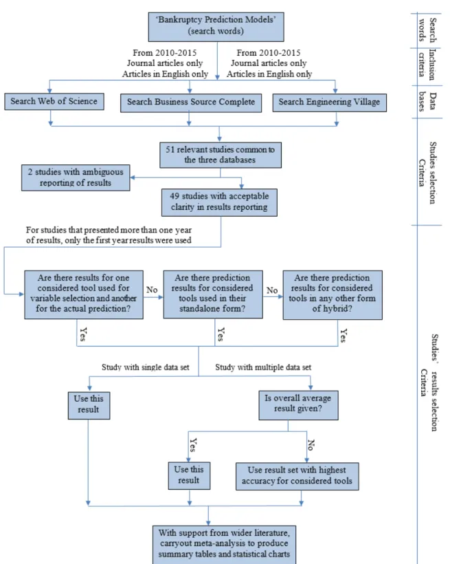
This study used a systematic review method to create a guideline for the selection of an appropriate tool for developing a bankruptcy prediction model (BPM). There are so many tools that can be used to develop a BPM that it is virtually impossible to review them all in one study. As a result, the two most popular statistical tools as noted by Balcaen and Ooghe (2006) in their comprehensive review of BPMs were reviewed: multiple discriminant analysis (MDA) and Logistic regression (LR). Also covered in this review are the most popular and promising artificial intelligence (AI) tools as advocated by Aziz and Dar (2006) in their comprehensive review, and Min et al. (2006) among others: artificial neural network (ANN), support vector machines (SVM), rough sets (RS), case based reasoning (CBR), decision tree (DT) and genetic algorithm (GA). A process flow of the methodology is presented in Figure 1.
(Khan et al., 2003). To improve validity of this study, only peer reviewed journal articles were considered since they are considered to be of high quality and their contribution considered as very valid (Schlosser, 2007).
Figure 1: Process flow of the methodology (the term ‘considered tool’ refers to the eight tools considered in this study).
databases were considered: Google Scholar; Wiley Interscience; Science Direct; Web of Science UK (WoS); and Business Source Complete (BSC). However, a careful observation revealed Google scholar produced an almost endless result and did not have the required filters to make it very efficient hence it was removed as it was unmanageable. Further observation revealed that (WoS) and BSC contained all the journal articles provided in Wiley and Science Direct; this is probably because the latter two are publishers while the former two are databases with articles from various publishers including the latter two. To increase the width of the search, Engineering Village (EV) database was added to WoS and BSC databases to perform the final search. EV was chosen because articles from the engineering world usually deal with BPM tools comprehensively.
The initial searches in the three databases (WoS, BSC and EV) showed that studies tend to use bankruptcy, insolvency and financial distress as synonyms for failure of firms. A search framework which captured all these words was thus designed with the following defined string (“Forecasting” OR “Prediction” OR “Predicting”) AND (“Bankruptcy” OR “Insolvency” OR “Distress” OR “Default” OR “Failure”).
To ensure high consistency and repeatability of this study, and consequently reliability and quality (Stenbacka, 2001; Trochim and Donnelly, 2006), only studies that appeared in the three databases were used; this ensured the eradication of database bias (Schlosser, 2007). These databases contain studies from all over the world hence geographic bias was also eliminated. Balcaen and Ooghe (2006) in their comprehensive review of statistical tools in 2006 noted that AI tools, mainly ANN, were gradually becoming adopted in BPM studies. With new tools emerging all the time, a four-year advance from 2006, which would have seen more use of AI tools, is how a start year of 2010 was chosen for this study. The end year is the year this paper was written, 2015.
Generally, the topic of articles that emerge from the search looked okay to determine which ones were fit for this study. However, this was not the case for all articles. Where otherwise, article’s abstract was read and, if necessary, introduction and/or conclusion were read. In some cases, the complete articles had to be read. Although language constraint is not encouraged in systematic review, it is sometimes unavoidable due to lack of funds to pay for interpretation services (Smith et al., 2011) as in the case of this study. Only studies written in English were thus used.
After eliminating unrelated studies that dealt with topics like credit scoring (e.g. Martens et al., 2010), policy forecasting (e.g. Won et al., 2012), or that did not use any of the tools reviewed (e.g. Martin et al., 2011), only 51 studies had a presence in the three data bases. Of these, two had great ambiguity in reporting their results hence were excluded, leaving 49 studies to be used as the sample. The ‘review studies’ in the search results (e.g. Sun et al., 2014) were not considered since original results from tools implementation were needed.
in consideration is used for variable selection and in turn used to hybridise the predicting tool, the result of such hybrid is used. Where the tools were used on more than one dataset and the results of each dataset was presented alongside the total average from all dataset, the total average results were used. In cases where average values were not given, the result set with the best accuracy for most/all of the tools in consideration in this study was used so as to give all tools a good chance of high accuracy. In cases where the results of more than a year of prediction were given, the results of the first year were used to allow for fair comparison since most BPM studies normally present first year results.
As required for systematic review, a meta-analysis was done with data synthesised using ‘summary of findings’ tables, statistical methods and charts (Khan et al., 2003; Higgins, 2008; Smith et al., 2011); with facts explained sometimes by employing quotes from especially the reviewed studies, and discussions backed up with a wider review of literature. Three summary of findings tables were provided in this study. Where there is not enough information from the reviewed studies regarding a certain criterion, results are discussed using the reviewed studies and wider literature. Opinions are only taken as facts in such cases if there are no opposing studies. This type of deviation from protocol for a valid reason is acceptable in systematic review (Schlosser, 2007). Finally, this review is used to create a guideline using a tabular framework for tool comparisons and a diagrammatic framework that clearly shows what situations/data characteristics/variable types etc. each discussed tool is best suited to. This will ensure developers can choose a tool based on what they have and/or intend to get rather than just arbitrarily.
3.0 The Tools
This study will review eight tools used to develop bankruptcy prediction models including: multiple discriminant analysis (MDA), Logistic regression (LR), artificial neural network (ANN), support vector machines (SVM), rough sets (RS), case based reasoning (CBR), decision tree (DT) and genetic algorithm (GA).
Multiple Discriminant Analysis: MDA uses a linear combo of variables, normally financial ratios, that best differentiate between failing and surviving firms to classify firms into one of the two groups. The MDA function, constructed usually after variable selection, is as follows:
Z = c1X1 + c2X2 + ……… + cnXn.
Where c1, c2, ………. cn, = discriminant coefficients; and X1, X2, …….. Xn = independent variables
MDA calculates the discriminant coefficients. The function is used to calculate a Z-score. A cut-off Z score is chosen based on status of sample firms
P1(Vi) = 1/[1 + exp - (b0+ b1Vi1+ b2Vi2 +…...+ bnVin)] = 1/[1 + exp - (Di)]
where P1(Vi) = probability of failure given the vector of attributes; Vi; Vij = value of attribute or variable j (j = 1, 2, ….., n) for firm i; bj = coefficient for attribute j; b0 = intercept; Di = logit of firm i.
The dependent variable P1 is expressed in binary form (0,1) (Boritz and Kennedy, 1995).
Neural Network: ANN was created to imitate how the neural system of the human brain works (Hertz et al., 1991) and was first applied to bankruptcy prediction by Odom and Sharda (1990). A typical ANN is a network of nodes interconnected in layers. There are various parameters, architectures, algorithms, and training methods that can be used to develop an ANN (Jo and Han, 1996) and choosing the best combination can be demanding.
Support vector machines: SVM employs a linear model to develop an optimal separating hyperplane by using a highly non-linear mapping of input vectors into a high-dimensional feature space (Shin et al., 2005; Ravi Kumar and Ravi, 2007). It constructs the boundary using binary class. The variables closest to the hyperplane are called support vectors and are used to define the binary outcome (failing or non-failing) of assessed firms. All other samples are ignored and are not involved in deciding the binary class boundaries (Vapnik, 1998). Like ANN, it has some parameters that can be varied for it to perform optimally (Dreiseitl and Ohno-Machado 2002).
Rough Sets: RS theory, discovered by Pawlak (1982), assumes that there is some information associated with all objects (firms) of a given universe; information which is given by some attributes (variables) that can describe the objects. Objects that possess the same attributes are indiscernible (similar) with respect to the chosen attributes. RS creates a partition in the universe that separates objects with similar attributes into blocks (e.g. failing and non-failing blocks) called elementary sets (Greco et al., 2001). Objects that fall on the boundary line cannot be classified because information about them is ambiguous. RS is used to extract the decision rules to solve classification problems (Ravi Kumar and Ravi, 2007; Greco et al., 2001).
Case Based Reasoning: CBR fundamentally differs from other tools in that it does not try to recognize pattern, rather it classifies a firm based on a sample firm that possess similar attribute values (Shin and Lee, 2002). It justifies its decision by presenting the used sample cases (firms) from its case library (Kolodner, 1993). It induces decision rules for classification.
Genetic Algorithm: GA is a searching optimization technique that imitates the Darwin principle of evolution in solving nonlinear, non-convex problems (Ravi Kumar and Ravi, 2007). It is effective at locating the global minimum in a very large space. It differs from other tools in that it simultaneously searches multiple points, works with character springs and uses probabilistic and not deterministic rules. GA can extract decision rules from data which can be used for classifying firms. It is applied to selected variables in order to find a cut-off score for each variable (Shin and Lee, 2002).
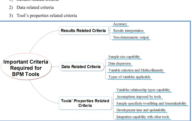
4.0 Important Criteria Required for Bankruptcy Prediction Model Tools
To be considered effective, there are many criteria that can be required to be satisfied by a tool when it is used to develop a bankruptcy prediction model (BPM). The set of criteria required usually depend on the situation and intention of the BPM developer. For example, a financier or client may simply be interested in the accuracy of a model. The BPM needed simply needs to be able to predict if a firm is financially healthy (unhealthy) enough to be granted (refused) a loan or contract, hence a highly accurate tool/technique is needed. A firm owner on the other hand is interested in result transparency as much as accuracy because he needs to know where/what the firm is going/doing wrong in order to know where rescue efforts need to be focused on. In such a case, a tool with high accuracy as well as result transparency will be needed to build the required BPM
Different researchers have used different criteria to develop their BPMs, however after a thorough and comprehensive review of the primary studies and other studies in the area, 13 criteria were identified to be the most common and important. Example of other reviewed studies include Tam and Kiang, (1992); Haykin, (1994); Zurada et al., (1994); Edum-Fotwe et al., (1996); Dreiseitl and Ohno-Machado, (2002); Min and Lee, (2005); Shin et al., (2005); Balcaen and Ooghe, (2006); Ravi Kumar and Ravi, (2007); Chung et al., (2008); Ahn and Kim, (2009); to mention a few. The identified 13 criteria are as follows:
1) Accuracy: This relates to the percentage of firms a tool correctly classifies as failing or non-failing.
2) Result transparency: This has to do with interpretability of a tool’s result.
3) Non-deterministic: The case where a tool cannot successfully classify a firm
4) Sample size: This refers to the sample size(s) suitable for a tool to perform optimally.
5) Data dispersion: This refers to ability of a tool to handle equally or unequally dispersed data
6) Variable selection: This refers to the variables selection methods required for optimum tool performance.
7) Multicollinearity: This refers to sensitivity of a tool to collinear variables.
8) Variable types: A tool’s capability to analyse quantitative and/or qualitative variables.
9) Variable relationship: This explains a tool’s limitation in analysing linear or non-linear variables
11) Sample specificity/overfitting: This is when the model developed from a tool performs well on sample firms but badly on validation data.
12) Updatability: The ease with which a tool’s model can be updated with new sample firms and its effectiveness afterwards
13) Integration capability: the ease with which a tool is hybridisable.
These 13 criteria can be grouped into three main categories as shown in Figure 2. These categories are:
1) Results related criteria 2) Data related criteria
3) Tool’s properties related criteria
Figure 2: Important criteria required for BPM tools
5.0 Results and Discussion
This section presents the results, analysis and discussion of the systematic review in form of summary of findings tables and statistical charts. The results are presented in relation to each identified criterion. The tables and charts compare the performance/ability of the tools as deduced from all the reviewed studies. The outcome is used to judge each tool based on the criterion in question. The criteria were assessed and discussed in the context of bankruptcy prediction models (BPM). For example, to assess the accuracy criteria of the tools, error cost had to be considered since it is an important aspect of accuracy assessment in the BPM research area.
statistical analysis regarding that criterion. The measure for exclusion was determined by calculating the average number of studies that provided information on the tools regarding the criterion in consideration; the tools with numbers well below average were excluded. This process, where employed, is clearly explained.
5.1
Results Related Criteria
5.1.1 Accuracy
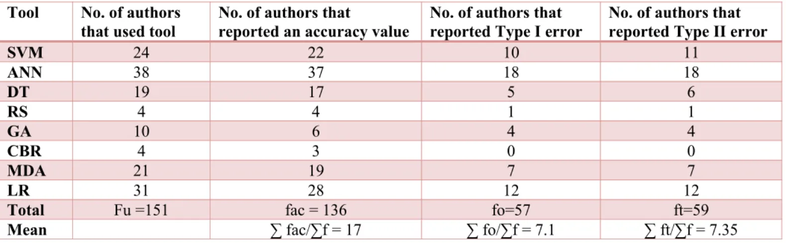
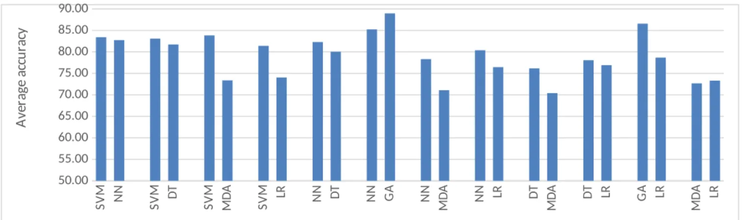
One of the main essences of using varying tools to develop BPMs is to increase accuracy of prediction. Figure 3 shows the mean average accuracy chart for each tool calculated from all the studies that gave an accuracy reading for the tool. The chart includes only the tools that had up to 17 studies that reported an accuracy value for them since the mean average of number of studies that reported accuracy value is 17 (Table 1). The chart clearly shows ANN and SVM to be the most accurate while MDA appears to be the least accurate. Table 2 is the first summary of findings table. It shows the accuracy value of each tool as reported in each study.
SVM NN DT MDA LR
70.00 72.00 74.00 76.00 78.00 80.00 82.00 84.00 86.00 A vg . of a cc ur ac y va lu e s
Figure 3: Overall average accuracy chart for each tool
Table 1: Summary statistics of the accuracy and error types of the tools
Tool No. of authors that used tool
No. of authors that
reported an accuracy value
No. of authors that reported Type I error
No. of authors that reported Type II error
SVM 24 22 10 11
ANN 38 37 18 18
DT 19 17 5 6
RS 4 4 1 1
GA 10 6 4 4
CBR 4 3 0 0
MDA 21 19 7 7
LR 31 28 12 12
Total Fu =151 fac = 136 fo=57 ft=59
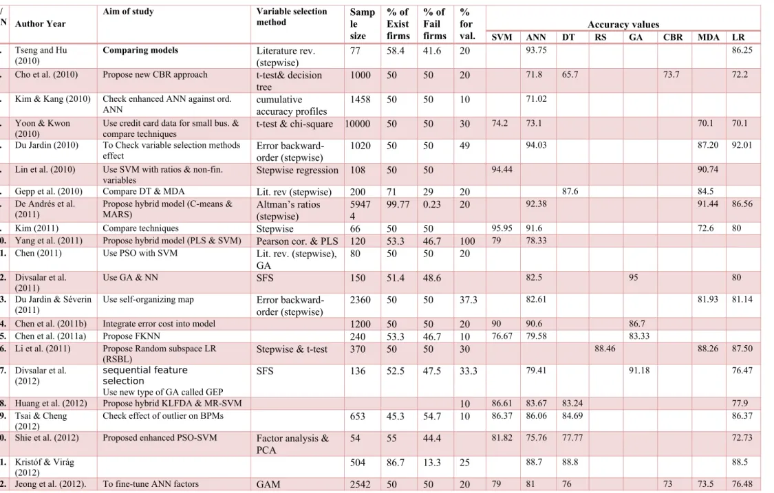
Table 2: Summary of reviewed studies aims, variable selection methods, sample characteristics and accuracy values S/
N Author Year
Aim of study Variable selection
method Sample
size % of Exist firms % of Fail firms % for
val. SVM ANN DT Accuracy valuesRS GA CBR MDA LR
1. Tseng and Hu
(2010)
Comparing models Literature rev.
(stepwise) 77 58.4 41.6 20
93.75 86.25
2. Cho et al. (2010) Propose new CBR approach t-test& decision
tree 1000 50 50 20
71.8 65.7 73.7 72.2
3. Kim & Kang (2010) Check enhanced ANN against ord.
ANN cumulative accuracy profiles 1458 50 50 10
71.02
4. Yoon & Kwon
(2010) Use credit card data for small bus. & compare techniques t-test & chi-square 10000 50 50 30 74.2 73.1 70.1 70.1
5. Du Jardin (2010) To Check variable selection methods
effect Error backward-order (stepwise) 1020 50 50 49
94.03 87.20 92.01
6. Lin et al. (2010) Use SVM with ratios & non-fin.
variables Stepwise regression 108 50 50 94.44 90.74
7. Gepp et al. (2010) Compare DT & MDA Lit. rev (stepwise) 200 71 29 20 87.6 84.5
8. De Andrés et al.
(2011) Propose hybrid model (C-means & MARS) Altman’s ratios (stepwise) 59474 99.77 0.23 20 92.38 91.44 86.56
9. Kim (2011) Compare techniques Stepwise 66 50 50 95.95 91.6 72.6 80
10. Yang et al. (2011) Propose hybrid model (PLS & SVM) Pearson cor. & PLS 120 53.3 46.7 100 79 78.33
11. Chen (2011) Use PSO with SVM Lit. rev. (stepwise),
GA
80 50 50 20
12. Divsalar et al.
(2011) Use GA & NN SFS 150 51.4 48.6 82.5 95 80
13. Du Jardin & Séverin
(2011) Use self-organizing map Error backward-order (stepwise) 2360 50 50 37.3 82.61 81.93 81.14
14. Chen et al. (2011b) Integrate error cost into model 1200 50 50 20 90 90.6 86.7
15. Chen et al. (2011a) Propose FKNN 240 53.3 46.7 10 76.67 79.58 83.33
16. Li et al. (2011) Propose Random subspace LR
(RSBL) Stepwise & t-test 370 50 50 30
88.46 88.26 87.50
17. Divsalar et al.
(2012) sequential featureselection
Use new type of GA called GEP
SFS 136 52.5 47.5 33.3 79.41 91.18 76.47
18. Huang et al. (2012) Propose hybrid KLFDA & MR-SVM 10 86.61 83.67 83.24 77.9
19. Tsai & Cheng
(2012) Check effect of outlier on BPMs 653 45.3 54.7 10 86.37 86.06 84.69 86.37
20. Shie et al. (2012) Proposed enhanced PSO-SVM Factor analysis &
PCA 54 55 44.4
81.82 75.76 77.77 72.73
21. Kristóf & Virág
(2012) 504 86.7 13.3 25 88.7 88.8 88.5
S/
N Author Year Aim of study Variable selection method Sample size % of Exist firms % of Fail firms % for
val. SVM ANN DT Accuracy valuesRS GA CBR MDA LR
23. Du Jardin & Séverin
(2012) To use Kohonen maptemporal accuracy to stabilize 81.3 81.2 81.6
24. De Andrés et al.
(2012)
To improve performance of classifiers 122 50 50 19.6 76.03 74.87
25. Zhou et al. (2012) To find the best variables for
accuracy Spearman correlation 50 50 10.8
71.1 67.8 75.6 64.4 54.4
26. Xiong et al. (2013) Use sequence on credit card data 70.94
27. Lee & Choi (2013) To do multi industry investigation t-test &correlation
analysis 1775 66.2 33.8 4.2
92 82.01
28. Tsai & Hsu (2013) Present met-learning framework
(hybrid) MC Avg. many 20
78.82 77.29 79.11
29. Callejón et al (2013) To increase predictive power of ANN 1000 50 50 20 92.11
30. Chuang (2013) To Hybridise CBR Multiple 321 86.9 13.1 90.1
31. Ho et al. (2013) Develop BPM for US paper
companies Lit rev (stepwise) 366 66.7 33.3 20 93
32. Arieshanti et al.
(2013)
To compare techniques Lit rev. (stepwise) 240 53.3 46.7 20 70.42 71
33. Kasgari et al. (2013) Compare ANN to other techniques Garson’s algorithm 135 52.5 47.5 25 94.11 88.57 91.43
34. Zhou et al. (2014) Propose new feature selection method GA 2010 50 50 75.6 50.67 71.72 73.99
35. Tsai (2014) To compare hybrids SOM 690 44.5 55.5 20 91.61 86.83 87.28
36. Yeh et al. (2014) To increase accuracy using RF&RS RF 220 75 25 33 94.58 92.95 91.55 96.99
37. Wang et al. (2014) Inject feature selection into boosting 132 50 50 10 79.99 75.69 75.99 73.90
38. Abellán & Mantas
(2014) To correctly use bagging scheme Lit. rev. (stepwise) 690 30 93.64
39. Tserng et al. (2014) To use LR to predict contractors
default 87 66.7 33.3
79.18
40. Yu et al. (2014) Produce BPM using ELM 500 50 50 33.3 93.2 86.5
41. Gordini (2014) Test GA accuracy & compare to other
techniques VIF & stepwise 3100 51.6 48.4 30
69.5 71.5 66.8
42. Heo & Yang (2014) To prove AdaBoost is right for
Korean construction firms 2762 50 50 20
73.3 77.1 73.1 51.3
43. Tsai et al. (2014) To compare classifier ensembles 690 44.5 55.5 10 86.37 84.38 86.37
44. Virág & Nyitrai
(2014) To show RS accuracy is competitive with SVM & ANN 156 50 50 25 89.32 88.03 89.32
45. Liang et al. (2015) To compare feature selections GA 688 50 50 10 91.77 91.63 92.98
46. Iturria1 & Sanz
(2015) To develop ANN BPM for US banks Mann-Whintney test & Gini index 772 50 50 13.5 89.42 93.27 77.88 81.73
47. Du Jardin (2015) To improve BPM accuracy beyond
one year 16880 50 50 50
80.8 80.1 80.6
48. Bemš et al. (2015). Introduce new scoring method called
Gini index Gini index 459 67 33 579
S/
N Author Year Aim of study Variable selection method Sample size
% of Exist firms
% of Fail firms
% for
val. SVM ANN DT Accuracy valuesRS GA CBR MDA LR
49. Khademolqorani et
Cor.: correlation ELM: extreme learning machine Exist firms: non bankrupt firms Fail firms: bankrupt firms FKNN: fuzzy k-nearest neighbour GAM: generalized additive model GEP: gene expression programming Lit. Literature KLFDA: kernel local fisher discriminant analysis
MARS: Multivariate Adaptive Regression Splines MC: meta classifier Rev.: review MR: manifold-regularized PCA: principal component analysis PLS: partial least squares PSO: particle swarm optimization RF: random forest RSBL: random subspace binary logit SFS:
sequential feature selection SOM: self-Organising maps Val.: ValidationVIF: variance Inflation Factor
Note: Bems et al. (2015) scoring methods results are not used as they will act as outliers in the computations of mean average and disadvantage accuracy results of tools that have them. Chen (2011) results were not clear enough to be included for computational analysis
The chart in Figure 4 shows a more direct comparison between pair of tools. It shows the average accuracy value calculated from studies that directly compared any pair of tools. The chart includes only the pairs that were compared in five or more studies since the mean average of the number of times any two tools were directly compared is 5.5 (see Table 3). To be more objective and fair in analysis, and to make a good critique, the pie charts in Figure 5 is produced to compare the percentage of studies that rated one tool as being more accurate than the other. It contains exactly the same pairs as Figure 4.
Figures 3, 4 and 5 all show that AI tools are more accurate than statistical tools except in Figure 5j where the number of studies that indicated that DT is more accurate than LR and vice versa are equal. Figures 4 and 5a-d clearly show SVM to be more accurate than any directly comparing tool though Figure 3, which is just the average accuracy of each tool, shows ANN to be more accurate. SVM apart, Figures 4 and 5e-h similarly show ANN to be more accurate than any comparing tool except for GA; with three against two studies confirming GA to be more accurate.
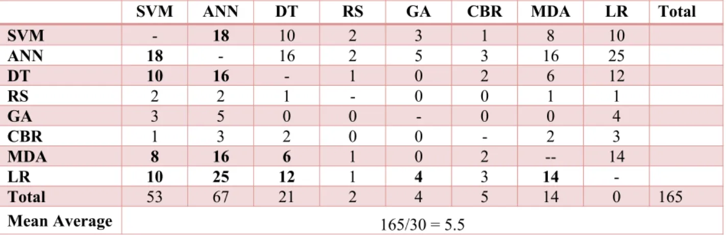
Table 3: Matrix of number of times studies directly compared pair of tools. The tools compared above the average number of comparisons are in bold
SVM ANN DT RS GA CBR MDA LR Total
SVM - 18 10 2 3 1 8 10
ANN 18 - 16 2 5 3 16 25
DT 10 16 - 1 0 2 6 12
RS 2 2 1 - 0 0 1 1
GA 3 5 0 0 - 0 0 4
CBR 1 3 2 0 0 - 2 3
MDA 8 16 6 1 0 2 -- 14
LR 10 25 12 1 4 3 14
-Total 53 67 21 2 4 5 14 0 165
Mean Average 165/30 = 5.5
S
V
M NN
S
V
M DT
S V M M D A S V
M LR NN DT
N N G A N N M D A N
N LR DT
M
D
A DT LR
G A LR M D A LR 50.00 55.00 60.00 65.00 70.00 75.00 80.00 85.00 90.00 A ve ra ge a cc u ra cy
Figure 4: Average accuracy results only from studies that directly compared pair of tools
16 g) h) d) b) e) f) c) a) k)
Figure 5: Pie charts that compare the percentage of studies that indicated one tool as being more accurate than the other.
A further examination of the five studies that compared the pair (ANN and GA) revealed they were written by two main set of authors. Of the five studies, only Chen et al. (2011a), which reported ANN and SVM as being more accurate than GA (see Table 2) could be said to have done a fair comparison since it produced the results for ANN and GA using the same features. Chen et al. (2011b) in their study developed a robust hybrid of GA and K-nearest neighbour (KNN) and compared it with other tools including ANN and SVM in their standalone form thus giving GA the advantage. Divsalar et al. (2011) ‘unfairly’ used a special version of GA called linear genetic programming (LGP) for comparison with normal ANN. Also, Divsalar et al. (2012) proposed a special version of GA called gene expression programming (GEP), thoroughly developed its BPM using all possible enhancements, and proved it was more accurate than models from other tools, including ANN developed with default settings.
Similarly, Kasgari et al. (2013), which included Divsalar as the second author, used the same data as Divsalar et al. (2012), proposed ANN for developing BPMs, thoroughly developed its model and proved it was more accurate than other tools, including GA. Besides, GA is well known to be more suited to the process of feature/variable selection because of its powerful global search hence its relatively infrequent use to develop BPMs (see Figure 6); it was used for this purpose in at least four of the primary studies (Chen, 2011; Jeong et al., 2012; Zhou et al., 2014; Liang et al. 2015) and other studies. Further “GA is a stochastic one. So, when using GA-based models on the same training samples twice, we may get two different models, and the decision on the same test sample may also be different. This stochastic characteristic of this method may be unacceptable for the decision makers or the analysts” (Zhou et al. 2014, p,252). SVM and ANN can thus be claimed to be more accurate. As noted in some of the reviewed studies (e.g. Virág and Nyitrai, 2014; Iturriaga and Sanz, 2015), this is in line with literature as it is mostly agreed that SVM and ANN are the most accurate tools for developing BPMs.
SVM NN DT RS GA CBR MDA LR
0.00 5.00 10.00 15.00 20.00 25.00 30.00
Fr
eq
u
en
cy
o
f
u
se
o
f
to
o
l (
%
)
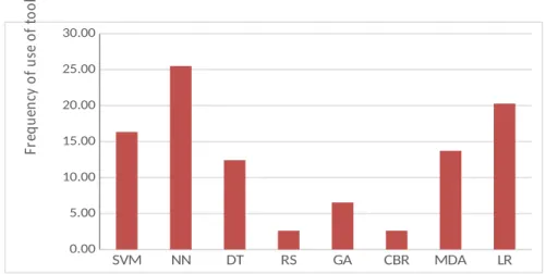
Figure 6: Percentage frequency of use of each tool
No study compared RS directly with GA. However, RS and ANN as well as SVM were compared directly in two studies and RS gave a slightly better result. Like the unfair cases with GA, Yeh et al. (2014) thoroughly developed many RS hybrid models using various enhancements and compared their average accuracy value to single accuracy values of separate hybrids of ANN and SVM. In the second study, Virág and Nyitrai (2014), working further from their previous study which confirmed SVM and ANN to be most accurate tools, decided to check why non-transparent tools (i.e. SVM and ANN) were more accurate than transparent tools like RS. They (Virág and Nyitrai 2014) initially concluded “there seems to be a kind of trade-off between the interpretability and predictive power of bankruptcy models” (p.420) so they tried to find out what to use with “RST technique in order to maximise the predictive power of the constructed model?” In other words, special effort was made to improve RS accuracy while SVM and ANN were used at default level; this obviously resulted in a biased result. Despite the effort, RS was only able to achieve the same accuracy as SVM and only a slightly higher accuracy than ANN (Table 3). Besides, Ravi Kumar and Ravi (2007) showed in their review that RS is not as accurate as claimed in many studies and Mckee (2003) reported a significantly reduced accuracy, compared to his previous study, when used with what was termed a ‘more realistic’ data. RS theory is difficult to implement hence its sparse usage (see Figure 6).
While DT’s average accuracy appears slightly higher than LR’s in Figure 4, Figure 5j shows that the number of studies that indicated DT to be more accurate than LR and vice versa are the same. DT has generally been confirmed to be less accurate than other AI tools like ANN and RS (Tam and Kiang, 1992; Chung and Tam 1992; McKee, 2000; Ravi Kumar and Ravi, 2007) except CBR; it (DT) has been classified as a somewhat weak classifier in one of the reviewed studies (Heo and Yang 2014). CBR is the overall least accurate tool. Of the four studies that used it, Chuang (2013) used it alone without comparison to any other tools. Jeong et al. (2012) and Bemš et al. (2015) showed that it was the least accurate when compared to SVM, DT, ANN, MDA and LR (Table 2). Only Cho et al. (2010), who presented an enhanced and hybridised CBR using DT and Mahalanobis distance, which was the aim of the study, was able to get a better accuracy figure for CBR (hybrid) than ANN, MDA and LR (Table 2). CBR’s low accuracy is a consequence of it not being able to handle non-linear problems and has been deemed by some as not suitable for bankruptcy prediction (e.g. Bryant, 1997; Ravi Kumar and Ravi, 2007). In the reviewed studies, Chuang (2013) noted that “one major factor for the poorer performance of a stand-alone CBR model lies in its failure to separate the more important “key” attributes from those less significant common attributes and to assign each key attribute with a different, corresponding weight” (p.184). No wonder it is very scarcely used for BPMs (see Figure 6). Of the two statistical models, LR is clearly the more accurate tool.
5.1.1.1 Error Cost
For accuracy ratings, error cost is a very important concept in bankruptcy prediction hence the tools must be appraised with regards to it. There are two types of error in bankruptcy prediction: type I and type II. Type I error is when a tool misclassifies a potentially bankrupt firm as being healthy. This is costlier as it could cause a financier to loan money to a failing firm and eventually lose the money, or it could make a firm relax when it is supposed to take active steps against insolvency. Type II error is when a tool misclassifies non-bankrupt firm as potentially bankrupt/failing. This error is less costly. This means a tool with relatively lesser type I error is more accurate. This, however, does not imply that type II error is unimportant as it could cost the firm its eligibility for loans, for example.
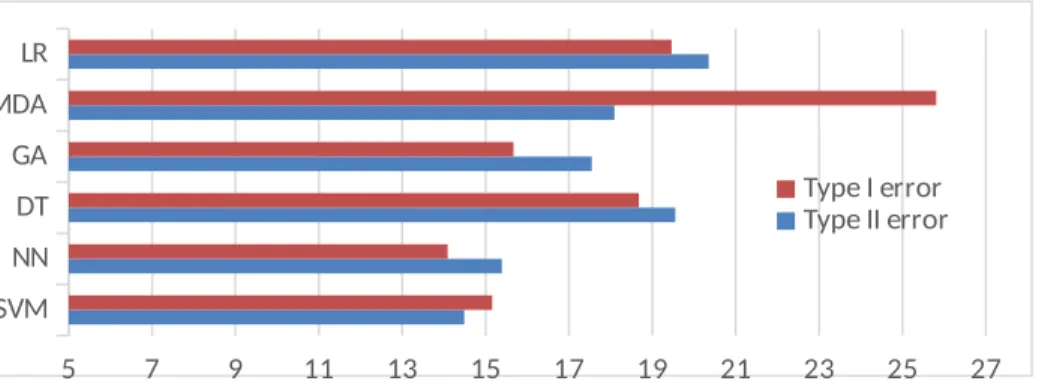
Since the mean average of frequency of reported types I and II errors are 7.36 and 7.63 respectively (Table 1), only the six tools that had up to 4 reporting studies and above were compared in the average types I and II error of tools chart in Figure 7. Four is deemed not too far from seven in this case so as to allow more tools to be compared. All error values are presented in Table 4. No study reported an error value for CBR while only one study reported for RS. Figure 7 shows that ANN has the least average type I error followed by SVM. Coupled with their high normal accuracy performance, they can be concluded to be the most accurate tools for bankruptcy prediction, followed by GA. DT and LR errors are again as close as their accuracies hence their total accuracy can be regarded to be of the same rank. However, MDA appears to be very poor with type I error hence its accuracy can be regarded as low. ANN, DT, GA and LR have better type I errors than type II errors and vice versa for SVM and MDA
SVM NN DT GA MDA LR
5 7 9 11 13 15 17 19 21 23 25 27
Type I error Type II error
Figure 7: Type I versus Type II error for each tool
5.1.2 Results Interpretation
nature of the tools as a major problem (Table 5 and Figure 8). Other studies have also pointed out that the results of ANN and SVM models are quite hard to understand in that weightings/coefficients they assign to the variables are illogical and very hard to interpret (Tam and Kiang, 1992; Shin et al., 2005; Chung et al., 2008; Ahn and Kim, 2009; Tseng and Hu, 2010).
Table 4: Summary of error types as reported for the tools by some of the authors
S/N Author Year SVM ANN DT RS GA MDA LR
Type I error Type II error Type I error Type II error Type I error Type II error Type I error Type II error Type I error Type II error Type I error Type II error Type I error Type II error
1. Kim & Kang (2010) 17.23 30.83
2. Yoon & Kwon (2010) 11.34 25.14
3. Du Jardin (2010) 4.72 7.22 16.8 8.8 9.58 6.4
4. Lin et al. (2010) 5.56 5.56
5. Kim (2011) 4.8 12.1 47.6 27.4 22 18.4
6. Yang et al. (2011) 8.93 17.2 16.07 26.56
7. Du Jardin & Séverin (2011) 17.95 16.82 18.41 17.73 18.18 19.55
8. Chen et al. (2011b) 15.7 4.3 12.2 6.7 17.1 9.7
9. Chen et al. (2011a) 26.55 18.96 18.52 21.71 14.94 17.02
10. Divsalar et al. (2012) 15.79 9.52 7.69 20
11. Tsai & Cheng (2012) 19.9 6.1 12.1 16.2 13.5 17.6 17.4 9.1
12. Shie et al. (2012) 16.7 17.65 22.23 25
13. Du Jardin & Séverin (2012) 20.1 17.4 22.1 15.5 20.1 16.6
14. De Andrés et al. (2012) 26.52 21.71 28.7 22.08 25.67 21.35
15. Lee & Choi (2013) 12.0 6.0 24 14
16. Tsai & Hsu (2013) 20.19 28.63 21.57 33.02 17.87 30.67
17. Kasgari et al. (2013) 5.0 7.14
18. Tsai (2014) 6.87 10.09 9.21 17.82 13.79 11.36
19. Yeh et al. (2014) 11.02 3.74 18.02 4.32 26.0 1.90 10.6 3.5
20. Wang et al. (2014) 21.55 18.19 20.62 27.69 23.10 24.74 26.38 25.38
21. Gordini (2014) 22.9 38.1 21.1 35.8 23.3 43.1
22. Iturria1 & Sanz (2015) 11.54 9.62 5.77 7.69 23.08 21.15 19.23 17.31
As noted by at least five of the reviewed studies (Table 5) and older studies (e.g. Ohlson, 1980; Tam and Kiang, 1992; Boritz and Kennedy, 1995; Balcaen and Ooghe, 2006 among others), the variable coefficients in LR represent the importance of variables thus its result is transparent and help users identify key areas of problem of a failing firm. As noted by at least five of the reviewed studies (Table 5) and some previous studies (Tam and Kiang, 1992; McKee, 2000; Greco et al., 2001; Shin and Lee, 2002; Shin et al., 2005; Ravi Kumar and Ravi, 2007), AI tools that generate decision rules for classification (i.e. RS, CBR, GA and DT) all produce explanatory results that can be easily interpreted and understood. It appears that for AI tools, the more accurate the tool, the less transparent the result (Figure 9). Nonetheless, McKee (2000) once spotted an inconsistency in a set of rules generated by RS in one of his previous co-authored studies.
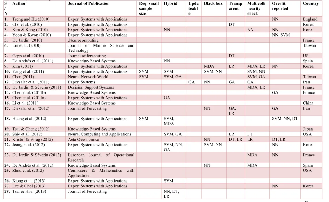
Table 5: Summary of tools that have been highlighted to be transparent, usable as hybrid, updatable, have overfitting problems etc., and year, country industry of the samples used in the reviewed studies
S / N
Author Journal of Publication Req. small
sample size
Hybrid Upda teabl e
Black box Transp arent Multicolli nearity check Overfit reported Country
1. Tseng and Hu (2010) Expert Systems with Applications NN England
2. Cho et al. (2010) Expert Systems with Applications DT Korea
3. Kim & Kang (2010) Expert Systems with Applications NN NN NN Korea
4. Yoon & Kwon (2010) Expert Systems with Applications NN, SVM
5. Du Jardin (2010) .Neurocomputing France
6. Lin et al. (2010) Journal of Marine Science and
Technology Taiwan
7. Gepp et al. (2010) Journal of forecasting DT US
8. De Andrés et al. (2011) Knowledge-Based Systems NN Spain
9. Kim (2011) Expert Systems with Applications MDA LR MDA, LR NN Korea
10. Yang et al. (2011) Expert Systems with Applications SVM SVM SVM, NN SVM, NN
11. Chen (2011) Neural Network World SVM SVM, GA SVM, GA Taiwan
12. Divsalar et al. (2011) Expert Systems GA NN GA GA Iran
13. Du Jardin & Séverin (2011) Decision Support Systems MDA, LR France
14. Chen et al. (2011b) Knowledge-Based Systems GA France
15. Chen et al. (2011a) Expert Systems with Applications GA
16. Li et al. (2011) Knowledge-Based Systems China
17. Divsalar et al. (2012) Journal of Forecasting NN GA,
LR GA Iran
18. Huang et al. (2012) Expert Systems with Applications SVM SVM,
MDA SVM, NN, DT
19. Tsai & Cheng (2012) Knowledge-Based Systems Japan
20. Shie et al. (2012) Neural Computing and Applications SVM, GA LR DT USA
21. Kristóf & Virág (2012) Acta Oeconomica NN DT, LR LR DT, LR
22. Jeong et al. (2012). Expert Systems with Applications SVM, NN,
GA
SVM, NN NN Korea
23. Du Jardin & Séverin (2012) European Journal of Operational
Research MDA NN France
24. De Andrés et al. (2012) Knowledge-Based Systems NN MDA Spain
25. Zhou et al. (2012) Computers & Mathematics with
Applications USA
26. Xiong et al. (2013) Expert Systems with Applications SVM
27. Lee & Choi (2013) Expert Systems with Applications NN Korea
28. Tsai & Hsu (2013) Journal of Forecasting NN, DT,
LR
S / N
Author Journal of Publication Req. small
sample size
Hybrid Upda teabl e
Black box Transp
arent Multicollinearity check
Overfit
reported Country
29. Callejón et al. (2013) International Journal of
Computational Intelligence Systems
multiple
30. Chuang (2013) Information Sciences CBR, RS,
DT CBR
31. Ho et al. (2013) Empirical Economics US
32. Arieshanti et al. (2013) TELKOMNIKA
(Telecommunication Computing Electronics and Control)
SVM, NN, LR
33. Kasgari t al. (2013). Neural Computing and Applications NN NN Iran
34. Zhou et al. (2014) International Journal of Systems
Science SVM SVM, NN,DT, GA SVM, NN SVM, NN, DT US
35. Tsai (2014) Information Fusion NN, DT,
LR
NN Australia
36. Yeh et al. (2014) Information Sciences SVM, NN,
DT, RS
37. Wang et al. (2014) Expert Systems with Applications US
38. Abellán & Mantas (2014) Expert Systems with Applications
39. Tserng et al. (2014) Journal of Civil Engineering and
Management
LR US
40. Yu et al. (2014) Neurocomputing SVM France
41. Gordini (2014) Expert Systems with Applications LR SVM, GA Italy
42. Heo & Yang (2014) Applied Soft Computing Korea
43. Tsai et al. (2014) Applied Soft Computing Japan
44. Virág & Nyitrai (2014) Acta Oeconomica SVM, NN, RS
45. Liang et al. (2015) Knowledge-Based Systems SVM, NN,
DT, GA China
46. Iturriaga & Sanz (2015) Expert Systems with Applications SVM, NN SVM, NN US
47. Du Jardin (2015) European Journal of Operational
Research France
48. Bemš et al. (2015). Expert Systems with Applications
49. Khademolqorani et al.
(2015) MathematicalEngineering Problems in NN NN, DT Iran
Figure 8: Percentage of studies that complained/noted the non-transparent nature of SVM and ANN
Kim (2011) and older studies (Altman, 1968; Taffler, 1983; Tam and Kiang, 1992; Balcaen and Ooghe, 2006) noted that although the MDA function makes MDA result look easily interpretable, the truth is that the variables’ coefficients in the function do not represent their importance, hence results are hard to interpret. Further, MDA sometimes yields a model with counter intuitive signs (Edum-Fotwe et al., 1996; Balcaen and Ooghe, 2006). One of many example models is Mason and Harris’ (1979) in which a negative sign was assigned to the profit before tax variable while representing firms with scores above cut-off as being healthy. This means profit is bad for a firm’s health! This is obviously incomprehensible.
Figure 9: Relationship between the accuracy and transparency of results of AI tools.
One relatively popular approach to transparency problem has been to use decision rules-generating tools to select variables and decide the importance of variables before using the very accurate black box tool for prediction. This, from the way it is explained, is obviously not the perfect answer as it sounds like using two separate tools for two different criteria. Kasgari et al. (2013, p.930) suggested that “to overcome this difficulty, the weights and biases are frozen after the network was well trained and then the trained MLP models are translated into explicit forms”, but did not explain how this is done.
5.1.3 Non-Deterministic Output
Unlike statistical tools and non-decision rules AI tools (i.e. ANN and SVM), AI tools that induce decision rules for classification can produce some non-deterministic rules i.e. rules that cannot be applied to a new object (firm) being assessed. The presence of non-deterministic rules for a new object can result into no classification (Ahn et al., 2000; McKee, 2000; Shin and Lee, 2002; Ravi Kumar and Ravi, 2007). Of the reviewed studies, Gordini (2014) highlighted GA as a tool that is synonymous with this problem. According to Shin and Lee (2002), as much as 46% of new cases might not be classified by these tools (GA was used in their study).
The non-deterministic problem is encountered in this group of tools because the set of rules extracted work like a multiple univariate system rather than a multivariate system. As a result, when any new case being assessed cannot satisfy any or all of the rules for one reason or the other, the non-deterministic problem arises. To curtail this problem, some studies have “reported that reduced data set (horizontally or vertically) is fed into neural network for complementing the limitation of RS, which finally produces full prediction of new case data” (Ahn et al., 2000, p. 68). Shin and Lee (2002) suggested the integration of multiple rules to solve the problem. For instance, if two of eight rules (two deterministic and six non-deterministic) show a new object as unhealthy, then the object is classified as unhealthy. Conclusively, it appears that there is no tool that clearly outperforms all other tools in relation to all result related criteria (Figure 10).
Figure 10: Performance of tools in relation to results related criteria. There is no one tool that satisfies all the results related criteria required to develop a robust prediction model.
5.2 Data Related Criteria
5.2.1 Data Dispersion and Sample Size Capability
Data dispersion, i.e. ratio of number of non-failing sample firms to failing sample firms, is known to be key to performance; the relative ease with which data on existing firms can be gathered usually makes them dominate data and reduce performance. According to Du Jardin (2015), this normally means that “data that characterized 25 High result
transparency
Fully Deterministic outputs High accuracy
CBR DT
MDA RS GA
ANN
SVM LR
failed firms would be hidden by those that represent non-failed firms, and therefore would become rather useless” (p.291) hence it is best to have equal dispersion (Jo et al., 1997).
MDA is quite sensitive to unequal dispersion (Balcaen and Ooghe, 2006). Compared to MDA, LR and Optimal Estimation Theory of ANN, are better with dispersion but ANN require the least dispersion at 20% failed firms before it could recognize pattern (Boritz et al., 1995; Du Jardin, 2015). However, no tool can perform reasonably well at this level of dispersion i.e. 20:80 (Boritz et al., 1995). The best option is to use equally dispersed data as most studies do. Most of the review studies have data dispersion ranging between 50-50 and 60-40 (Figure 11) with nearly half using equally dispersed data (Table 2).
The sample size available for analysis can also influence the performance of a tool and should thus be given serious consideration before selecting a tool. At least three of the reviewed studies (Tseng and Hu, 2010; De Andrés et al. 2012; Zhou et al. 2014), and other studies (Haykin, 1994; Min and Lee, 2005; Shin et al., 2005; Ravi Kumar and Ravi, 2007) clearly indicated that ANNs and MDAs need a large training sample in order to reasonably recognize pattern and provide highly accurate classification. According to Haykin (1994), the minimum number of sample firms required to train an ANN network is ten times the weights in the network with an allowable error margin of 10%, i.e. over 1000 sample firms will be required to properly train a standard ANN to make it fit for generalization. This is not too commonly implemented in many ANN studies (Shin et al., 2005) as is evident in this study (Figure 12). However, Lee et al (2005) were able to show that ANNs can still perform reasonably well (better than statistical models) with a small number of sample firms provided ‘a target vector is available’. Like with ANN, a primary study (Tseng and Hu, 2010) and another study (Ravi Kumar and Ravi, 2007) have reported DT and LR to require a large data set to perform well.
CBR, RS and SVM can handle small data size (Jo et al., 1997; Olmeda, and Fernández, 1997; Ravi Kumar and Ravi, 2007). Although Buta (1994) claimed that CBR’s accuracy increases with increase in data size, Ravi Kumar and Ravi (2007) made it clear that it cannot handle very large data. At least four of the reviewed studies confirmed SVM’s special ability to perform well with a small training dataset (Table 5), with Zhou et al. (2014) 26 Figure 12: Proportion of studies that used less or
more than the 1000 firms sample size for ANN Figure 11: Proportion of studies that used
noting in their wide experiment that “most SVM-based models can still keep higher performance as the size of training samples decreases. It demonstrates that SVM models can keep good performance with small training samples, which has been proved in many other applications also” (p.248). In Yang et al.’s (2011) experiment, they showed that for their SVM, “the support vector number is 33 and 35 … This shows that only 33 and 35 samples from the total of 120 samples are required to achieve the appropriate identification” (p.8340). In fact, Shin et al., (2005) did prove that SVM performs better and optimally with small training data sets as against a large one and fairs better than ANN only when a small data set is used to train both. This SVM’s advantage is confirmed in older studies as well (e.g. Min and Lee, 2005; Shin et al., 2005; Ravi Kumar and Ravi, 2007).
5.2.2 Variable Selection, Multicollinearity and Outliers
Statistical tools, especially LR, are highly sensitive and reactive to multicollinearity hence an effective method of choosing non-collinear variables is normally employed for them (Edmister, 1972; Joy and Tollefson, 1975; Back et al., 1996; Lin and Piesse, 2004; Balcaen and Ooghe, 2006). Multicollinearity can easily lead to unstable performance and inaccurate results (Edmister, 1972; Joy and Tollefson, 1975; Balcaen and Ooghe, 2006). Before the emergence of AI tools, the most common variable selection method is the stepwise method because of its effectiveness in avoiding collinear variables (Altman, 1968; Back et al., 1996; Jo et al., 1997; Lin and Piesse, 2004). Its common use, over quarter of the studies used it, is usually to allow fair comparison with statistical tools.
The reviewed studies (Chen, 2011; Chen et al., 2011b; Yang et al., 2011; Liang et al., 2015) and other previous studies (Altman et al., 1994; Jo and Han, 1996; Chung et al., 2008) clearly indicate that AI tools, apart from CBR, are less sensitive to multicollinearity and can perform well with almost any variable selection method. CBR’s performance decreases with increased number of variables (Chuang, 2013). On the other hand, some studies have claimed the higher the number of variables (usually when the multitude of variables available are used without selecting special ones), the better for ANN and GA (Chen, 2011; Chen et al., 2011b; Liang et al., 2015). In fact, Liang et al. (2015), who particularly investigated the effect of variable selection, concluded that “performing feature [variable] selection does not always improve the prediction performance” (p.289) of AI tools. However, Huang et al. (2012) feel removing irrelevant variables’ can improve performance. Although Liang et al. (2015) found no best variable selection method in their study, they and Back et al. (1996) recommended GA as the best selection method for AI tools. Overall, it is not uncommon to use a decision rule generating AI tool to select variables for another AI tool as in some of the reviewed studies (Chen, 2011; Jeong et al., 2012; Zhou et al., 2014; Liang et al. 2015) and older studies (Wallrafen et al., 1996; Back et al., 1996; Ahn and Kim, 2009).
Although outliers can cause problems for any tool, LR has been particularly noted to be extremely sensitive to outliers in at least two of the reviewed studies (Kristóf and Virág, 2012; Tsai and Cheng 2012). Outlier effects are normally reduced by normalising variables by industry average (McKee 2000). Such normalization has however been found to reduce accuracy of models (Tam and Kiang, 1992; Jo et al., 1997).
5.2.3 Types of Variables Applicable
This criterion was not explicitly considered by the primary studies hence only the wider literature was used to discuss it. Although the vast majority of BPM studies use quantitative variables, usually in form of financial ratios, the need for qualitative/explanatory/managerial variables use, as noted in many studies, cannot be overemphasized (Argenti, 1980; Zavgren, 1985; Keasey and Watson, 1987; Abidali and Harris, 1995; Alaka et al., 2016 among others). MDAs can use only quantitative variables (Altman, 1968; Taffler, 1982; Odom and Sharda, 1990; Agarwa and Taffler, 2008; Chen, 2012; Bal et al., 2013 and more) while LR can use both (Ohlson, 1980; Keasey and Watson, 1987; Lin and Piesse, 2004; Cheng et al. 2006; Tseng and Hu, 2010).
ANNs and SVMs can use mainly quantitative variables but can also use qualitative variables converted to quantitative variables using means such as the Likert scale (Cheng et al. 2006; Lin, 2009; StatSoft, 2014). All AI tools that yield the ‘if… then,’ decision rules for bankruptcy prediction, inclusive of RS, DT, CBR and GA, use qualitative variables and need quantitative variables to be converted to qualitative such as ‘low, medium, high’ etc. before they can be analyzed making them suitable for use of combined variables (Quinlan; 1986; Dimitras et al., 1999; Shin and Lee, 2002; Ravi Kumar and Ravi, 2007; Martin et al., 2012). The conversion is however not carried out by the AI and “involves dividing the original domain into subintervals which appropriately reflect theory and knowledge of the domain” (McKee, 2000, p. 165).
5.3 Tools’ Properties Related Criteria
5.3.1 Variables Relationship Capability and Assumptions Imposed by Tools
Many independent variables used with BPM tools do not possess a linear relationship with the dependent variable (Keasey and Watson, 1991; Balcaen and Ooghe, 2006). Three of the reviewed studies (Du Jardin and Séverin, 2011; Divsalar et al., 2012; Du Jardin and Séverin, 2012) highlighted that MDA and LR require a linear and logistic relationship respectively between dependent and independent variables. This means important predictor variables with non-linear relationship to dependent variable will cause MDA to perform poorly. LR can solve logistic and non-linear problems (Tam and Kiang, 1992; Jackson and Wood, 2013). From this review, it appears all AI tools, except CBR (Chuang, 2013), can solve non-linear problems as identified by about a
quarter of the reviewed studies (e.g. Divsalar et al., 2011; Du Jardin and Séverin, 2011, 2012; Chen et al., 2011b; Shie et al., 2012; Kasgari t al., 2013; Zhou et al., 2014; Yeh et al., 2014; among others).
Du Jardin and Séverin (2011) and other studies (Coats and Fant 1993; Lin and Piesse, 2004; Balcaen and Ooghe, 2006; Chung et al., 2008; among others) have shown that statistical tools require data to satisfy certain restrictive assumptions for optimal performance. Some of these assumptions include multivariate normality of independent variables, equal group variance-covariance, groups are discrete and non-overlapping etc. (Ohlson, 1980 Joy and Tollefson, 1975; Altman, 1993; Balcaen and Ooghe, 2006). All these restrictive assumptions can barely be satisfied together by one data set hence are violated in many studies (Richardson and Davidson, 1984; Zavgren, 1985; Chung et al., 2008). Nonetheless LR is deemed relatively less demanding compared to MDA (Altman, 1993; Balcaen and Ooghe, 2006; Jackson and Wood, 2013). On the other hand, none of the reviewed studies noted any restrictive assumptions on data for AI tools. This is because they look to extract knowledge from training samples or directly compare a new case to cases in the case library (Coats and Fant 1993; Shin and Lee, 2002; Lin, 2009; Jackson and Wood, 2013).
5.3.2 Sample Specificity/Overfitting Tendency and Generalizability of Tools
The common use of stepwise variable selection method and mainly financial ratios as variables for statistical tools sometimes lead to a sample specific model where the model performs excellently on the samples used to build it but woefully on hold out samples thereby possessing low generalizability (Edmister, 1972; Lovell, 1983; Zavgren, 1985; Agarwal and Taffler, 2008). LR nonetheless has a relatively reasonable generalizability (Dreiseitl and Ohno-Machado, 2002).
The equivalent of sample specificity in AI tools is called overfitting and is a common problem. There is also underfitting which is vice versa of overfitting. It is now a norm to avoid this problem (in statistical and AI tools) by testing models on a validation sample (and re-model if necessary) as indicated in most of the reviewed studies (Figure 13a). Over a third of the reviewed studies also pro-actively identified this problem early (Figure 13b) and considered it from the initial model development stage. Overfitting and underfitting are not necessarily caused by variable selection method or variable types in the case of AI tools. Apart from the case of CBR, it is generally known that the longer (shorter) the decision rules, the more the possibility of overfitting (underfitting) (Clark and Niblett, 1989; Brodley and Utgoff, 1995; Ravi Kumar and Ravi, 2007; Ren, 2012). CBRs tend not to overfit because they simply match a new case to one or more very similar cases in their library (Watson, 1997). CBR however has poor generalization but that is due to its poor accuracy (Ravi Kumar and Ravi, 2007).
Figure 13: Proportion of studies that identified overfitting problem early and those that solved the problem using validation sample
Overfitting is a known problem of ANN and is as a result of overtraining the network (Min and Lee, 2005; Cheng et al. 2006; Ahn and Kim, 2009; Tseng and Hu, 2010; Jackson and Wood, 2013). Suggestions on how to construct more generalizable networks in ANN are given by Hertz et al. (1991). Overfitting (underfitting) in SVM is caused by a too large (small) upper bound value, usually denoted with ‘C’ (Min and Lee, 2005; Shin et al., 2005). Thus, finding the optimum number of training and optimum C value for ANN and SVM respectively is key to their optimum performances. The notion that the structural risk minimization (SRM) used by SVM helps it to reduce the possibility of overfitting and increases generalization is not well proven according to Burges (1998). However, the tendency of overfitting in SVM is lower than in ANN and MDA (Cristianini and Shawe-Taylor, 2000; Kim, 2003; Shin et al., 2005).
5.3.3 Model Development Time, Updatability and Integration Capability with other Tools
Although the reviewed studies did not really touch on training times, past studies have noted that training AI tools, especially ANN and GA, can take a relatively longer time compared to statistical tools. This is because of the iterative process of finding the best parameters for AI tools (Jo and Han, 1996; Min and Lee, 2005; Ravi Kumar and Ravi, 2007). ANN architectures normally require many training cycles and GAs search for global optimum, while locating and negating local minima, make them (ANN and GA) take time for model development (Fletcher and Goss, 1993; Shin and Lee, 2002; Ravi Kumar and Ravi, 2007; Chung et al., 2008). For SVM, the polynomial function takes a long time but its RBF function is quicker (Kim, 2003; Huang et al., 2004). RS however does not take very long to train (Dimitras et al., 1999).
As noted in the reviewed studies, CBR and GA create the most updatable BPMs (Table7). CBR is easy to update and quite effective after an update since all it takes is to simply add new cases to its case library and prediction of a new case is done by finding the most similar cases(s) among all cases, old and new, in the library (Bryant, 1997; Ahn and Kim, 2009). An attempted update of a statistical BPM can lead to much reduced accuracy (Mensah, 1984; Charitou et al., 2004). ANNs can be adaptively updated with new samples since they are known to be robust on sample variations (Tam and Kiang, 1992; Altman, 1993; Zhang et al., 1999). However, if the
30 b)
situations of the new cases are significantly different for the ones used to build the model, then a new model must be developed (Chung et al., 2008). RS is particularly very sensitive to changes in data and can really be ineffective after an update with data that has serious sample variations (Ravi Kumar and Ravi, 2007)
AI tools are more flexible and allow integration with other tools better than statistical tools do. This is evident from the reviewed studies as more of the studies that used AI tools produced hybrids with them than those that used statistical tools (Figures 14a and b). The review clearly indicates that effective hybrids perform better than standalone tools (Tsai, 2014; Zhou et al., 2014; Iturriaga and Sanz, 2015), and “usually outperforms even the MLP [a type of ANN] and SVM procedure” (Iturriaga and Sanz 2015, p.2866). This is also confirmed in older studies (Jo and Han, 1996; Jeng et al., 1997; Ahn et al., 2000; Ahn and Kim, 2009). “However, these hybrid models consume more computational time” (Zhou et al. 2014, p.251) and “it is unknown which type of the prediction models by classifier ensembles and hybrid classifiers can perform better”. (Tsai 2014, p.50)
Figure 14: Proportion of studies that integrated AI or statistical tools to form a hybrid
6.0 The Proposed Model
Figure 15 presents a diagrammatic framework, gotten from the result of this review, which serves as a guideline for a BPM developer to select the right tool(s) that is best suited to available data and BPM preference criteria. Virtually all tools that are used for developing BPMs can successfully make predictions. However, some tools are more powerful in relation to certain criteria than others (see Table 6).
The framework clearly shows that to get the best performance from a BPM, the developing tool should be selected based on the output criteria preferences and the characteristics of data available. The framework is a very good starting point for any BPM developer and will ensure tools are not selected arbitrarily to the disadvantage of the developer. It will also ensure the final user of the BPM, having communicated his requirements to the model developer, gets the most appropriate BPM. For example, a BPM developer that considers accuracy as the highest preference because of his client’s requirements, but has a very small dataset
31 b)