Volume 2008, Article ID 287061,13pages doi:10.1155/2008/287061
Research Article
Feature Point Detection Utilizing the Empirical
Mode Decomposition
Jesmin Farzana Khan,1Kenneth Barner,2and Reza Adhami1
1Department of Electrical and Computer Engineering, University of Alabama in Huntsville, Huntsville, AL 35899, USA 2Department of Electrical and Computer Engineering, University of Delaware, Delaware, DE 19716, USA
Correspondence should be addressed to Jesmin Farzana Khan,[email protected]
Received 22 June 2007; Revised 18 January 2008; Accepted 3 March 2008
Recommended by Ray Zhang
This paper introduces a novel contour-based method for detecting largely affine invariant interest or feature points. In the first step, image edges are detected by morphological operators, followed by edge thinning. In the second step, corner or feature points are identified based on the local curvature of the edges. The main contribution of this work is the selection of good discriminative feature points from the thinned edges based on the 1D empirical mode decomposition (EMD). Simulation results compare the proposed method with five existing approaches that yield good results. The suggested contour-based technique detects almost all the true feature points of an image. Repeatability rate, which evaluates the geometric stability under different transformations, is employed as the performance evaluation criterion. The results show that the performance of the proposed method compares favorably against the existing well-known methods.
Copyright © 2008 Jesmin Farzana Khan et al. This is an open access article distributed under the Creative Commons Attribution License, which permits unrestricted use, distribution, and reproduction in any medium, provided the original work is properly cited.
1. INTRODUCTION
There are a wide variety of methods reported in the literature for interest point and corner detection in grey-level images. Current detection methods can be categorized into three types: contour-based, parametric model-based, and intensity-based methods. Contour-based methods first extract contours and then search for maximal curvature or inflexion points along the contour chains, or carry out some polygonal approximation and then search for intersection points. Contour-based methods have existed for some time [1–6]. This work proposes a contour-based technique that is inspired by the fact that there is a correspondence between the wavelet decomposition and the EMD of a given signal, for example, the wavelet decomposition of a signal gives higher energy where the signal contains information, while the intrinsic mode function (IMF) of the EMD shows higher frequency content at the same locations. Corner detection schemes using the wavelet transform (WT) are popular due to the fact that the WT is able to decompose an input signal into smooth and detailed parts by low-pass and high-pass filters at multiresolution levels [7]. In this manner, local deviations are easily captured at various detailed
decompo-sition levels. Several wavelet-based approaches are reported in [8–15].
Parametric model methods fit a parametric intensity model to the signal. They often provide subpixel accuracy, but are limited to specific types of interest points, for example, L-corners. A parametric model is used in [16–19]. Intensity-based methods compute a measure that indicates the presence of an interest point directly from the grey values. This type of detector does not depend on edge detection or mathematical models [20–30].
that true corners result in stronger tangent variations, the 1D EMD is utilized to decompose the 1D tangent angles and capture the irregular angle variations. Finally, the locations of the true feature points are identified by comparing the local frequency content of the first intrinsic mode function (IMF) of the 1D decomposed signal with a predefined threshold.
A requirement for good feature point detection is that the detector be invariant to image transformations and yields the same detected points for different viewpoints. The proposed method is largely invariant to significant affine transformations including large rotations and scale changes. Such transformations introduce significant changes in point locations as well as in the scale and the shape of the neighborhoods of interest points. Our approach addresses these problems simultaneously and offers invariance to geometric transformation. Thus, the points detected in the original image and points detected after the transformation of the image commute. Such points have often been called invariant feature points in the literature, though in principle they change covariantly with the transformation. Thus, even though the regions themselves are covariant, the normalized image pattern they cover and the feature descriptors derived from them are typically invariant.
In this paper, we evaluate the proposed method utilizing the “repeatability” [34] criteria, which directly measures the quality of the detected feature points for tasks such as image matching, object recognition, and 3D reconstruction. It is complementary to localization accuracy, which is relevant for tasks such as camera calibration and 3D reconstruction of specific scene points. Repeatability and localization are conflicting criteria; smoothing improves repeatability but degrades localization [35]. Repeatability explicitly compares the geometrical stability of the detected interest points between different images of a given scene taken under varying viewing conditions. An interest point is “repeated” if the 3D scene point detected in the first image is also accurately detected in the transformed image. The proposed detector is compared to five existing methods that have been shown to yield good results. Utilizing repeatability, the proposed method is shown to yield comparable to improved results.
The remainder of the paper is organized as follows: the proposed corner detection algorithm is described in
Section 2. Experimental results along with the compari-son to five other existing methods are demonstrated in
Section 3. Concluding remarks and recommendations for future improvement are given inSection 4.
2. PROPOSED ALGORITHM
2.1. Motivation
It is reported that the wavelet transform is a robust scheme for feature points detection due to its ability to decompose an input signal into smooth and detailed components. This fact motivates the consideration of the EMD for interest. The EMD technique was developed recently to analyze the time-frequency distribution of nonlinear and nonstationary data. The EMD is an adaptive decomposition through which any
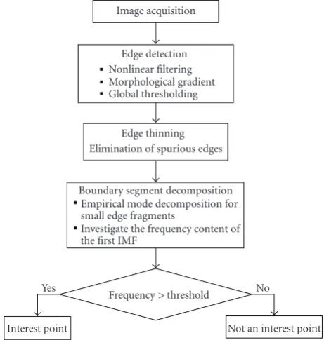
Image acquisition
Edge detection Nonlinear filtering Morphological gradient Global thresholding
Edge thinning Elimination of spurious edges
Boundary segment decomposition Empirical mode decomposition for small edge fragments
Investigate the frequency content of the first IMF
Yes No
Frequency>threshold
Interest point Not an interest point Figure1: Block diagram of the proposed algorithm.
signal can be decomposed into its IMFs that provide well-defined instantaneous frequency information of the signal.
Unlike Fourier or wavelet techniques, the EMD does not assume the form of the underlying oscillatory modes or basis functions. For a given signal, the wavelet decomposition is less compact and physically meaningful than the EMD results [36]. The EMD decomposition method is adaptive and highly efficient. Since the decomposition is based on the local characteristic of the data, it is applicable to nonlinear and nonstationary processes. Experimental results presented here show that, for feature point selection, the EMD is also robust and gives better performance than wavelet approaches.
In the proposed approach, we select the feature points from the edges and, to make the selection process robust, we use morphological edge detection along with edge thinning. The methodology of the proposed method is to use an eigenvector of the covariance matrix for a boundary point over a small region of support (ROS) on a small boundary segment as a curvature function for feature point detection. Thus, we perform the EMD on small edge fragment after edge detection and thinning operations. The derived edge detection and thinning method is used in lieu of traditional method, such as Canny edge detection [35], because it returns edge segments rather than contiguous edge lines, which is beneficial in feature point detection.
2.2. The EMD-based feature point determination
A block diagram of the proposed algorithm is shown in
open-close and close-open filters [37]. Next, a morphological gradient operator is applied to the blurred image, which gives symmetric edges between foreground and background regions, and the resulting image is converted to binary edge map by a global nonhistogram-based thresholding technique [38]. A new edge thinning algorithm is applied to this binary image to obtain fine, narrow, and well-defined object boundaries. Next, a novel technique for selecting feature points from object boundaries based on the EMD is employed. In this work, we represent edges as a set of straight or curved line fragments that are used to extract local curvature by analyzing the eigenvectors of covariance matrices using the 1D EMD. Specifically, each small 2D boundary segment is transformed to a 1D θ −
P representation (where θ is the tangent angle variations of the arc length, P, along the object’s boundary) that is decomposed using the 1D EMD. At the true feature points, the first IMF signal of the EMD shows distinctly higher frequency contents than at the points which carry less, or no, information. Thus, points where the frequency measure of the first IMF signal is greater than a predefined threshold are set as interest points. The following subsections discuss each step of the algorithm in detail.
2.2.1. Morphological edge detection
Most classical edge detectors such as Laplacian of Gaussian (LoG) [39] and Canny [35] are based on differential opera-tions and hence are primarily effective in detecting step edge. In contrast to classical techniques, morphological operations [37] are highly effective in detecting different types of features. In this paper, a morphological scanning edge detector (MSED) [32] is applied. The operator is insensitive to skew and orientation, free from artifacts introduced by both global and fixed size block-based local thresholding, and robust to noise. It has been reported that edge features [40] can better handle lighting and scale variations in natural scene images than texture features [41, 42]; therefore, we choose to use an edge-based approach in this study.
An efficient morphological edge detection scheme is applied to the the intensity image, I, as follows [32]. The image I is first blurred (to reduce false edges and oversegmentation) using open-close and close-open filters [37]. The final blurred image,Ib, is the average of the outputs of these two filters,
Ib= B
BIo c+B BIc o
2 , (1)
where Bis the 3×3 eight-connected structuring element, andBIo andBIc denote the opening and closing ofI by the structuring elementB, respectively. Next, the morphological gradient operator [43] is applied to the blurred image Ib, resulting in an image,
Ies=δB
Ib−εBIb, (2) whereδBandεBand are the dilation and erosion operators, respectively, utilizing the 3×3 eight-connected structuring elementB. The morphological gradient is an edge-strength
extraction operator that gives symmetric edges between the foreground and background regions. The resulting image, Ies, is then thresholded to obtain a binary edge mask. A global
nonhistogram-based thresholding technique is incorporated rather than local (adaptive) thresholding [38]. The threshold level,γ, is set as,
γ= Ies·c
c , (3)
where · denotes pixel-wise multiplication and c =
max(|g1∗∗Ies|,|g2∗∗Ies|); alsog1=[−101];g2 =[−101]T,
and ∗∗ denotes 2D linear convolution. The binary edge imageIeis then given by,
Ie=
1 ifIes> γ,
0 otherwise. (4)
To thin the edges, the morphological edge map is scanned along the horizontal and vertical directions to reduce the width of the edges to a single pixel by through erosion. During horizontal scanning, all the nonzero neighborhood pixels of a nonzero edge pixel in a horizontal window 1×wh are set to 0. The resulting image isIhe,
ifIexi,yj=/0,
then ⎧ ⎪ ⎪ ⎪ ⎨ ⎪ ⎪ ⎪ ⎩ Ihe
xi,yj=Iexi,yj
Ihe
xi,yk=0; fork∈k /=j
j−wh
2 , j+ wh
2
.
(5)
Similar operations in the vertical direction yield
ifIexi,yj=/0,
then ⎧ ⎪ ⎪ ⎪ ⎨ ⎪ ⎪ ⎪ ⎩ Ihe
xi,yj=Iexi,yj
Ihe
xi,yk=0; fork∈k /=j
j−wh
2 , j+ wh
2
.
(6)
The maximum ofIheandIveis set as the thinned binary edge
image,Ite, resulting from the edge thinning operation,Ite =
max(Ihe,Ive). The imageItemay still contain isolated noisy
spurious edges. To remove these edge, segments of length less thanN are deleted. Letnsequential points describe an edge segment P in Ite such that P = {pi = (xi,yi);i =
1, 2, 3· · ·n}. Then Ite
xi,yi=0 forxi,yi∈P,n≤N. (7)
The resulting final binary edge image, Ifte, contains 1pixel
width boundaries in the image.
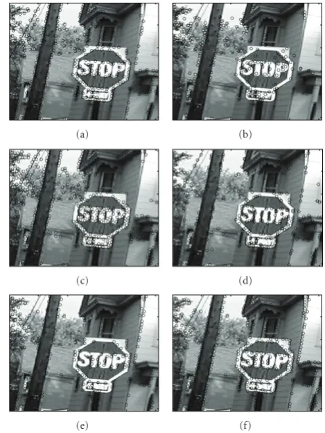
As an example, the intensity image, the morphological edge strength extracted image, gradient image after global thresholding, and the final edge image after thinning and elimination spurious edges are shown in Figures2(a),2(b),
(a) (b)
(c) (d)
(e) (f)
Figure 2: (a) Intensity image, (b) morphological edge strength image, (c) morphological edge after thresholding, (d) final edge image after thinning, (e) Canny edge image for a low threshold and (f) Canny edge image for a high threshold.
The reason for not using an existing edge detection method, for example, Canny edge detection method [35], is that Canny’s method yields extraneous boundaries as shown inFigure 2(e). Though for a higher threshold Canny method gives fewer boundaries. In using this approach, however, the threshold needs to be determined by hand for each image. Moreover, even by setting a different threshold it does not return edge segments but rather long continuous edges and connected edges between two objects. The methodology of the proposed algorithm is to use the covariance matrix for a boundary point over a small region of support (ROS), on a small boundary segment, as a curvature function for feature point detection. It has been found that the morphological framework and edge thinning scheme yields edge segments, which facilitates the extraction of feature points.
2.2.2. Empirical mode decomposition
The EMD decomposes a signal into a finite number of (zero mean) frequency and amplitude modulated signals called IMFs. The first IMF contains the highest local frequencies of oscillation while the final IMF, or the residue, contains a single extremum, a monotonic trend, or simply a constant.
The basic idea embodied in the EMD analysis, as introduced by Huang et al. [31], is to allow for an adaptive and unsupervised representation of the intrinsic components of linear and nonlinear signals, based purely on the properties observed in the data without appealing to the concept of stationarity. Although the EMD is a relatively new data analysis technique, its power and simplicity have encouraged its application in a myriad of fields, including almost all areas of signal processing, image processing, computer vision, and medical analysis [44–48].
2.2.3. Feature points extraction
After obtaining the binary edge image, Ifte, the feature
points along the boundaries of objects must be determined. If the boundary of an object involves both straight lines and circular arcs, spurious corners may be detected at circular arcs by boundary-based approaches. To overcome this shortcoming, Tsai et al. [33] introduced the eigenvalues of a covariance matrix for a boundary point, over a small region of support (ROS) on a small boundary segment, as a curvature function for feature point detection. We adopt this approach in order to retain the robust merits of covariance matrix in feature point detection. However, instead of using multiple eigenvalues, the principal eigenvector is used in this work, because the dominant orientation of any pixel in the local neighborhood can be either denoted as the argument of the principal eigenvector or by using the ratio between two eigenvalues. This technique is applied to each segment of the 2D boundaries of the edge image and feature points are extracted from each segment. As this approach considers a small boundary segment as a new curvature function for feature detection, image noise and quantization effect are readily eliminated.
The 1D wavelet transform has been utilized as a robust scheme in feature point detection due to its excellent local deviations capturing capability. In this work, the 2D boundaries of an object are initially transformed to a 1Dθ−P representation. Then, 1Dθ−P signal is used as input for the 1D EMD to detect the local deviations as measured by the number of zero crossing points of the first IMF. In the following, we present the procedure of finding the tangent angle of the boundary point.
2.2.4. 1Dθ−prepresentation of boundary segment
From the binary edge image,Iftethex-ycoordinates of each
point of a boundary segment of an object are first extracted into an array. Let a boundaryPof an object be described byn sequential digital points,P= {pi=(xi,yi);i=1, 2, 3· · ·n}, where pi+1 is adjacent topionP. LetNs(pi) denote a small
boundary segment of P with point pi is at the center of Ns(pi) over the ROS between pointspi−sandpi+sfor some integers. That is,Ns(pi)= {pj:j∈ {i−s,i+s}}. Therefore, the covariance matrixM(pi) for pointpiis estimated by the boundary points coordinates withinNs(pi) [49];
Mpi=
m11 m12
m21 m22
where,
m11=
1 2s+ 1
j=i+s
j=i−s x2j
−x2i,
m22=
1 2s+ 1
j=i+s
j=i−s y2
j
−y2
i,
m12=m21=
1 2s+ 1
j=i+s
j=i−s xjyj
−xiyi,
xi= 1
2s+ 1 j=i+s
j=i−s xj,
yi= 1 2s+ 1
j=i+s
j=i−s yj,
(9)
where xi and yi are the geometrical center of Ns(pi). The covariance matrix M(pi) is a 2 ×2 symmetric, positive semidefinite matrix. The eigenvaluesλ1andλ2ofM(pi) are
the solutions of the characteristic equation DET(M(pi)−D), whereDis unit matrix. The corresponding eigenvectorsE1
andE2 represent the tangent (major axis) and the normal
(minor axis) directions for pointpiover the segmentNs(pi), respectively. Therefore, the tangent angle of pointpi, denoted byθ(pi), is simply defined as follows:
tanθpi=
λ1−m11
m12
,
θpi=arctan
λ1−m11
m12
.
(10)
In general, the magnitude of θ(pi) is between −π/2 andπ/2. However, in order to avoid the large variation for two adjacent boundary points due to quantization effects [8, 10], θ(pi) is defined as between 0 and π/2. That is, θ(pi)= |arctan((λ1−m11)/m12)|. However, ifm12equals to
0, thenθ(pi) is set toπ/2 to avoid divided by zero situations. Therefore, the angle of a boundary pointpican be calculated by the eigenvectorE1ofM(pi) and the above expression for
θ(pi).
2.2.5. Detection procedure
Consider ann1-point digital boundary,P = {pi = (xi,yi);
i = 1, 2, 3· · ·n1}, traversing points (x1,y1), (x2,y2),. . .,
(xn1,yn1), and circumventing the boundary in the
counter-clockwise direction.For eachpisequence, there corresponds a 1Dθ−Psignal,θ(pi), 1D wavelet signal,Y(pi), and a 1D first IMF signal of the EMD,X(pi).
As an example, we have chosen a binary image with one object.Figure 3(a)shows a binary image of an artificial “h”-shape object. Figure 3(b) presents the edge image of that object with one boundary involving n1 = 273 boundary
points. The character “+” inFigure 3(b)denotes the starting boundary point (x1,y1) and the arrow indicates the direction
of boundary following. The corresponding 1D θ − P representation of the object boundary,θ(pi) is shown at the top ofFigure 3(c), which is used as an input signal to both the
100 80 60 40 20 90 70 50 30 10 (a) 100 80 60 40 20 90 70 50 30 10 (b) −1
−0.5 0 0.5 1 −2 −1 0 1 2 0 0.5 1 1.5 2 300 250 200 150 100 50 0 300 250 200 150 100 50 0 300 250 200 150 100 50 0 (c) 100 80 60 40 20 90 70 50 30 10
Final points from wavelet decomposition (d) 100 80 60 40 20 90 70 50 30 10
Final points from EMD
(e)
Figure3: (a) Binary image of letter “h”; (b) starting boundary point and direction of boundary following; (c) the 1Dθ−Prepresentation of the “h”-shape object (top), haar wavelet decomposition at first decomposition level (middle), and the first IMF of the EMD (bottom); (d) feature points obtained from the location of distinct wavelet coefficients; and (e) feature points obtained from the frequency content of the first IMF of the EMD.
image of letter “h” based on the 1D wavelet decomposition method are shown inFigure 3(d).
In the EMD case, the first IMF shows distinctly higher frequency content at true feature points than at straight lines. The algorithm for finding true interest points makes four passes through the IMF signal. First, points are selected if they exceed a minimum number of zero crossings around them. Second, if two selected points are adjacent then one is deleted based on the concentration of zero crossings. During the third pass, the selected points that are not locally maximum in the original intensity image in its 3×3 neighborhood are deleted. In the final pass, the subset of pixels are kept such that the minimum distance between any pair of points is larger than a given threshold.
LetZ(pi) be the set of zero-crossing points of the IMF aroundpi:
Z(pi)=pj:Xpj−1
X(pj+1)<0
;
forj∈
i−Wz
2 ,i+ Wz
2
, (11)
where Wz defines window centered at pi. If for a point, the number of zero crossings is greater than a predefined threshold, thz (in our work, the threshold is 1/3 of the maximum number of zero crossings in the IMF signal), that point is likely a feature point. This is the first selection of the feature points from the object boundary, which forms the set F1⊂P:
F1=
pi:Z(pi)>thz
=pi=(xi,yi);i=1, 2, 3,· · ·,n2:n2< n1
, (12)
wheren1 is the number of all the boundary points and n2
is the number of selected points after discarding redundant points.
To discard redundant points, we check whether several neighboring points have the same number of zero-crossing points over aWs = 1×11 size window, and we keep the points among those that have the most concentrated zero-crossing points. Hence for each point over the windowWz, we calculate the sum of the distances from all the zero-crossing points to the point under consideration,pi,
S(pi)=
j=i+Wz/2
j=i−Wz/2
|pi−pj|. (13)
If F2 ⊂ F1 is the set of feature points after discarding
redundant points fromF1, thenF2∩F1is the set of discarded
points:
F2∩F1=
pj:Z(pj)=Z(pi) andS(pj)=/minS(pj) forj∈
i−Ws
2 ,i+ Ws
2
,
F2=
pi=(xi,yi);i=1, 2, 3,· · ·,n3:n3< n2< n1
, (14)
where n3 is the number of selected points after discarding
redundant points fromF1.
Figure4: A synthetic image.
Finally, from the points inF2, we retain those points that
are locally maximum in their Wm = 3×3 neighborhood with the restriction that the distance between any two feature points is larger than a given threshold (this is set to 5 pixels in our experiment). Thus,F3⊂F2is the set of feature points
that are locally maximum in the edge image,Ifte, andFf ⊂F3
is the final set of feature points after discarding those closely spaced points:
F3=
pi=(xi,yi) :Ifte(xi,yi)= max
{j∈i−Wm/2,i+Wm/2}
Ifte(xj,yj)
,
F3=
pi=(xi,yi);i=1, 2, 3· · ·n4:n4< n3< n2< n1
, (15)
where n4 is the number of selected points after discarding
redundant points fromF2:
Ff =pi:pi−pi−1>5 pixels, andpi−pi+1>5 pixels
, Ff =pi=xi,yi;i=1, 2, 3· · ·n5:n5< n4< n3< n2< n1
, (16)
where n5 is the number of selected points after discarding
redundant points fromF3.
Following the above procedure, the extracted final feature points, Ff for the artificial “h”-shape object are shown in
Figure 3(e). By comparing the final feature point extraction results shown in Figures3(d) and3(e), it can be said that the IMF is richer in containing useful information about the original signal than the wavelet decomposition. That is, the EMD determined feature points are found at all the curvatures of the object whereas the wavelet decomposition approach misses some curvatures.
For an image with more than one object and objects with complicated shape, we perform the EMD on each edge fragment to extract local curvature following the above procedure. Thus, we find feature points for each fragment of edge independently and the final feature points are the accumulation of all the points obtained from all the edge boundary segments.
3. EXPERIMENTAL RESULTS
(a) (b)
(c) (d)
(e) (f)
Figure 5: Feature points detected in the synthetic image by (a) Harris method (b) Lowe’s method, (c) Tomasi’s method, (d) Loupias’s technique, (e) Yeh’s algorithm, and (f) proposed technique.
transformations, the original images are scaled, rotated, and sheared. Stability to image noise is also tested. Additionally, the repeatability rates of five interest point detectors are compared with the presented method under different image rotation and scale changes. Finally, analysis is performed on parameter sensitivity of the algorithm.
For comparison, we have chosen five detectors that are reported to offer good performance. Among the five chosen detectors, Harris’s [24], Lowe’s [30], and Tomasi’s methods [25] are intensity-based methods.These are chosen because Harris’s method has been reported to be better than any other detector, Lowe’s algorithm also known as SIFT (scale invariant feature transform) is the best scale invariant detector, and Tomasi’s detector is the best for tracking applications. The other two detectors [13, 15] are chosen because (1) they are contour-based methods like the proposed method and (2) they use the wavelet decomposition.
The above mentioned methods and the proposed algo-rithm are first applied to a synthetic image consisting of horizontal, vertical, and slanted lines; and different types of corners. As shown in Figure 4, this synthetic image contains both prominent and faint edges. The feature points detected by Harris’s, Lowe’s, Tomasi’s, Loupias’s, and
(a) (b)
(c) (d)
(e) (f)
Figure6: Feature points detected by (a) Harris method (b) Lowe’s method, (c) Tomasi’s method, (d) Loupias’s technique, (e) Yeh’s algorithm, and (f) proposed technique.
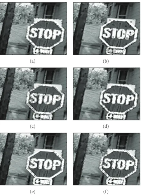
Yeh’s methods are shown in Figures 5(a),5(b),5(c), 5(d), and5(e), respectively. The interest points extracted by the presented algorithm are given inFigure 5(f). Even though the proposed method identifies fewer number of feature points than some of the presented approaches, it is interesting to observe that these feature points are distributed along all edges, boundaries, and corners of interest.This is true for prominent boundaries and edges, as well as subtle interior edges. Many object corners and boundaries are missed by the other methods, especially the faint interior edges. Thus, the proposed method has produced the most judicious feature points, placing them logically along the structures of interest. Simulation results for the five methods on a real image are presented inFigure 6. For the reference image shown in
Figure 2(a), feature points extracted by Harris’s approach, Lowe’s procedure, Tomasi’s method, Loupias’s technique, and Yeh’s algorithm are shown in Figures 6(a),6(b),6(c),
6(d), and 6(e), respectively. The points detected by the presented method are given inFigure 6(f). From this figure, it can be seen that points selected by the proposed method cover all the curvatures of object boundaries and yields the most true corner points.
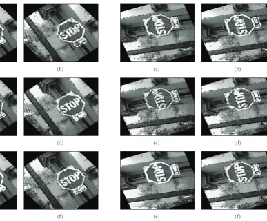
To evaluate detector rotation invariance, Figures7 and
(a) (b)
(c) (d)
(e) (f)
Figure7: Feature points detected in 40◦rotated image by (a) Harris method (b) Lowe’s method, (c) Tomasi’s method, (d) Loupias’s technique, (e) Yeh’s algorithm, and (f) proposed technique.
the reference image. Figures 7(f)and 8(f)give the results of the proposed method, where the rotation angle for the images are 40◦ and 110◦for the images in Figures7and8, respectively. The performance of Harris’s, Lowe’s, Tomasi’s, Loupias’s, and Yeh’s methods are given in Figures7(a),7(b),
7(c), 7(d), and 7(e), respectively, for 40◦ rotation and in Figures 8(a), 8(b),8(c),8(d), and 8(e), for 110◦ rotation. From the figures, it is observed that Harris’s, Lowe’s, and the proposed method give the best result for both rotations. The performance of Tomasi’s technique is better than Loupias’s and Yeh’s methods.
The effect of image scale change on detection result is tested and demonstrated in Figures 9 and 10. The points detected by the proposed technique are shown in Figures
9(f) and 10(f), where the scale changes are 1.5 and 3.4, respectively. Points detected by Harris’s, Lowe’s, Tomasi’s, Loupias’s, and Yeh’s methods are presented in Figures9(a),
9(b),9(c),9(d), and 9(e), respectively for the scale change 1.5 and in Figures 10(a), 10(b), 10(c), 10(d), and 10(e), respectively for the scale change 3.4. It can be seen from the figures that all the methods are scale invariant.
To evaluate the functioning of all five detectors as affine invariant systems, nonuniform scaling is applied in some directions to have shearing in the reference image shown in
(a) (b)
(c) (d)
(e) (f)
Figure 8: Feature points detected in 110◦ rotated image by (a) Harris method (b) Lowe’s method, (c) Tomasi’s method, (d) Loupias’s technique, (e) Yeh’s algorithm, and (f) proposed technique.
Figure 2(a).Figure 11(f)displays the feature points detected in the sheared image by the proposed method. The results of detection by Harris’s, Lowe’s, Tomasi’s, Loupias’s, and Yeh’s methods are presented in Figures11(a),11(b),11(c),11(d), and11(e), respectively. By examining the figure, it can be said that the proposed method performs satisfactorily for detecting interest points from the sheared image as well.
To check the performance with noise, we have added Gaussian noise to the original image. For a noisy image with a SNR of 25 dB,Figure 12(f)presents the points detected by the proposed method. The performance of Harris’s, Lowe’s, Tomasi’s, Loupias’s, and Yeh’s methods are given in Figures
12(a), 12(b), 12(c), 12(d), and 12(e), respectively, for the same level of noise. The results demonstrate that except for Tomasi’s technique, the other five methods work well in the presence of noise.
(a) (b)
(c) (d)
(e) (f)
Figure 9: Feature points detected in 1.5 times scaled image by (a) Harris method (b) Lowe’s method, (c) Tomasi’s method, (d) Loupias’s technique, (e) Yeh’s algorithm, and (f) proposed technique.
points detected in those images under different geometric and photometric transformations. We take into account only the points located in the part of the scene present in both images. Measuring the repeatability rate within 1.5 pixels or less, the probability that two points are accidentally within the error distance is negligible.
We first compare the detectors for image rotation followed by scale change and additive noise. The repeatability rate as a function of the angle of image rotation is displayed in Figure 13(a). The rotation angles vary between 0◦ and 180◦. Under repeatability, Harris’s and Lowe’s methods give the best results for all rotations, where these algorithms obtain a repeatability rate of about 82% and 77%, respec-tively. From the observation of the plot of the repeatability rate with image rotation, the proposed technique does not outperform Harris method or SIFT algorithm, but it yields a repeatability rate of about 70% for all rotations. Notably, it offers better performance than Tomasi’s, Loupious’s, and Yeh’s techniques, where these approaches offer a repeatability rate of about 60%, 50%, and 40%, respectively.
Figure 13(b)shows the repeatability rate as a function of scale changes. The results show that all the detectors are scale sensitive except Lowe’s method. As the name implies, the SIFT algorithm proposed by Lowe offers the best performance with scale change. This method is the least
(a) (b)
(c) (d)
(e) (f)
Figure 10: Feature points detected in 3.4 times scaled image by (a) Harris method (b) Lowe’s method, (c) Tomasi’s method, (d) Loupias’s technique, (e) Yeh’s algorithm, and (f) proposed technique.
dependent on the change in scale. The Harris’s, Tomasi’s, and the proposed detectors give reasonable results, with the repeatability rate as a decreasing function of scale change. Laopious’s and Yeh’s methods are very sensitive to scale change and the results of these methods are hardly usable.
To study repeatability in the presence of image noise, the repeatability rate is displayed as a function of SNR. For performance evaluation with noise, the SNR is varied from 35 dB to 21 dB and the results are displayed inFigure 13(c). All the detectors give reasonable results in the additive noise cases, with the exception of Tomasi’s method. Harris’s and Laopious’s methods give the best results followed by the proposed and then by Lowe’s, Yeh’s, and Tomasi’s techniques. The proposed method obtains a repeatability rate of nearly 70% for all levels of noise considered.
For the evaluation of detection performance, the feature points extracted by the proposed method and the five other algorithms are presented for two more images in Figures14
(a) (b)
(c) (d)
(e) (f)
Figure11: Feature points detected in sheared image by (a) Harris method (b) Lowe’s method, (c) Tomasi’s method, (d) Loupias’s technique, (e) Yeh’s algorithm, and (f) proposed technique.
of the image. Most importantly, the proposed method covers all the curvatures of object boundaries and yields at the true features, that is, the edges, ridges, and corners. Accordingly, the extracted points detect the structure of the scene and lead to a complete image representation.
Analysis is done on the sensitivity to algorithm param-eters. Most existing interest point detectors depend on the choice of some parameters. The threshold in Harris’s method is chosen by trial and error depending on the problem at hand. The number of points detected by the SIFT algorithm varies significantly with the change in image intensity. For example, for the image used in the paper, the number of detected feature points by SIFT is 862, if the input image is not normalized and it is 363 if the same input image is normalized.
In the proposed method there is one threshold, thzwhich determines the set of the first selection of the interest points such that any point will be selected if it exceeds a minimum number of zero crossings around it. This threshold is not a function of image intensity, rather it is the function of number of zero-crossing points of an IMF and thus, it is different for each edge segment of an image. In the paper, this threshold has been set as the 1/3 of the maximum number of zero crossings present in an IMF signal and this choice
(a) (b)
(c) (d)
(e) (f)
Figure12: (a) Feature points detected in noisy image with SNR = 25 dB by (a) Harris method (b) Lowe’s method, (c) Tomasi’s method, (d) Loupias’s technique, (e) Yeh’s algorithm, and (f) proposed technique.
is independent of the image. As this threshold selects the preliminary set of the feature points, any value which is equal to or smaller than the value yields the same result. Choosing the value for this threshold is not stringent and has minor effect on the final set of extracted feature points. Because the preliminary feature points selected by this threshold go through three more passes for the redundant points to be discarded. The two more thresholds in those passes define the size of the local neighborhood of a pixel. Thus, those thresholds are not a function of image intensity, but rather image size. The value of those two thresholds chosen in the paper work well for most of the images we come across in practice. We have tested Harris method and the proposed algorithm for different values of the threshold, thz.Table 1gives the number of detected points for Harris and the proposed method as a function of the threshold (thz =Threshold×(1/3) of the maximum number of zero crossings).
20 30 40 50 60 70 80 90 110 100
180 160 140 120 100 80 60 40 20 0
Rotation (degrees) Harris
SIFT EMD
Tomasi Laopious Yeh (a)
10 20 30 40 50 60 70 80 90
4 3.5 3 2.5 2 1.5 1
Change in scale Harris
SIFT EMD
Tomasi Laopious Yeh (b)
45 50 55 60 65 70 75 80 85 90 95
36 34 32 30 28 26 24 22 20
SNR (dB) Harris
SIFT EMD
Tomasi Laopious Yeh (c)
Figure13: Plot for the repeatability rate as a function of (a) rotation angle, (b) change in scale, and (c) noise level.
(a) (b)
(c) (d)
(e) (f)
Figure 14: Feature points detected in the second image by (a) Harris method (b) Lowe’s method, (c) Tomasi’s method, (d) Loupias’s technique, (e) Yeh’s algorithm, and (f) proposed technique.
any feature point detector. Though the proposed technique does not outperform Harris method or SIFT algorithm, it yields better results than Tomasi’s, Loupious’s, and Yeh’s techniques. Notably, it offers better performance than the
(a) (b)
(c) (d)
(e) (f)
Figure15: Feature points detected in the third image by (a) Harris method (b) Lowe’s method, (c) Tomasi’s method, (d) Loupias’s technique, (e) Yeh’s algorithm, and (f) proposed technique.
100 80 60 40 20
90 70 50 30 10
(a)
100 80 60 40 20
90 70 50 30 10
(b)
Figure16: Interest points detected from the binary image of letter “h” by (a) the SIFT algorithm and (b) the proposed algorithm.
Table1: Effect of threshold on the number of detected points.
Threshold 1 0.9 0.8 0.7 0.6 0.5 0.4 0.3 0.2 0.1 Harris
method 303 308 314 322 326 334 346 362 377 391 Proposed
method 303 303 303 303 303 303 303 303 303 303
boundaries for further processing. As an example, for a binary image, interest points should not be found in the uniform region of constant intensity, that is, either in the background or foreground. Rather interest points must lie only on the edges. As shown in Figure 16, for the binary image of the letter “h”, the SIFT algorithm detects feature points in the uniform region. But the proposed method, as a contour-based technique, extracts interest points only from the edges, which signifies the performance variation of different algorithms depending on the types of image and/or applications.
4. CONCLUSION
This research presents a robust, rotation invariant, and scale-invariant corner detection scheme for images based on the morphological edge detection, the eigenvectors of covariance matrices for boundary segment points, and the 1D EMD. We modify an existing morphological edge detection scheme to yield thin edges and eliminat spurious edges resulting from the background. The main contribution of this work is the utilization of the first IMF of EMD of the 1D θ−P signal of the edge to localize true corner points on boundary contours. Under appropriate image resolution and region of support, the proposed approach precisely captures the true corner points and is free from false alarms on circular arcs for both simple and complicated objects in varying rotation, scale conditions, and noise contaminations.
The interesting attribute of this technique is that it does not detect feature points globally. Rather it detects feature points locally, based on the neighboring characteristics of a small edge segment. This results in the presented method being more independent of image transformation than the other five methods considered for comparison. Thus, interest points detected by the proposed method are largely independent of the imaging conditions; that is, detected points are geometrically stable.
Additionally, for the proposed technique we do not need either to implement the computational extensive 2D EMD or to calculate all the IMFs of 1D EMD. Only the first IMF of 1D EMD is required. Experimental results also suggest that the proposed 1D EMD-based corner detection approach is stable and efficient. The proposed method is a generic concept and can find its application in many matching and recognition problems.
REFERENCES
[1] A. Bandera, C. Urdiales, F. Arrebola, and F. Sandoval, “Corner detection by means of adaptively estimated curvature func-tion,”Electronics Letters, vol. 36, no. 2, pp. 124–126, 2000. [2] R. Rattarangsi and R. T. Chin, “Scale-based detection of
corners of planar curves,” IEEE Transactions on Pattern Analysis and Machine Intelligence, vol. 14, no. 4, pp. 430–449, 1992.
[3] R. Horaud, F. Veillon, and T. Skordas, “Finding geometric and relational structures in an image,” inProceedings of the 1st European Conference on Computer Vision (ECCV ’90), pp. 374– 384, Antibes, France, April 1990.
[4] E. Shilat, M. Werman, and Y. Gdalyahu, “Ridge’s corner detec-tion and correspondence,” inProceedings of IEEE Computer Society Conference on Computer Vision and Pattern Recognition (CVPR ’97), pp. 976–981, San Juan, Puerto Rico, USA, June 1997.
[5] F. Mokhtarian and R. Suomela, “Robust image corner detec-tion through curvature scale space,” IEEE Transactions on Pattern Analysis and Machine Intelligence, vol. 20, no. 12, pp. 1376–1381, 1998.
[6] A. Pikaz and I. Dinstein, “Using simple decomposition for smoothing and feature point detection of noisy digital curves,”
IEEE Transactions on Pattern Analysis and Machine Intelligence, vol. 16, no. 8, pp. 808–813, 1994.
[7] A. Bruce and H. Y. Gao,Applied Wavelet Analysis with SPLUS, Springer, New York, NY, USA, 1996.
[8] Y.-N. Sun, J.-S. Lee, and C. T. Tsai, “Multiscale corner detection by using wavelet transformation,”IEEE Transactions on Image Processing, vol. 4, no. 4, pp. 100–104, 1995.
[9] C.-H. Chen, J.-S. Lee, and Y.-N. Sun, “Wavelet transformation for gray-level corner detection,”Pattern Recognition, vol. 28, no. 6, pp. 853–861, 1995.
[10] A. Quddus and M. M. Fahmy, “Fast wavelet-based corner detection technique,”Electronics Letters, vol. 35, no. 4, pp. 287– 288, 1999.
[11] A. Quddus and M. Gabbouj, “Wavelet-based corner detection technique using optimal scale,” Pattern Recognition Letters, vol. 23, no. 1–3, pp. 215–220, 2002.
[12] J. P. Hua and Q. M. Liao, “Wavelet-based multi scale corner detection,” inProceedings of the 5th International Conference on Signal Processing (ICSP ’00), pp. 341–344, Beijing, China, August 2000.
[13] E. Loupias, N. Sebe, S. Bres, and J.-M. Jolion, “Wavelet-based salient points for image retrieval,” in Proceedings of IEEE International Conference on Image Processing (ICIP ’00), vol. 2, pp. 518–521, Vancouver, BC, Canada, September 2000. [14] M. S. Lew, E. Loupias, T. S. Huang, Q. Tian, and N. Sebe,
“Image retrival using wavelet-based salient points,”Journal of Electronic Imaging, vol. 10, no. 4, pp. 835–849, 2001.
[16] K. Rohr, “Recognizing corners by fitting parametric models,”
International Journal of Computer Vision, vol. 9, no. 3, pp. 213– 230, 1992.
[17] R. Deriche and T. Blaszka, “Recovering and characterizing image features using an efficient model based approach,” in
Proceedings of IEEE Computer Society Conference on Computer Vision and Pattern Recognition (CVPR ’93), pp. 530–535, New York, NY, USA, June 1993.
[18] S. Baker, S. K. Nayar, and H. Murase, “Parametric feature detection,”International Journal of Computer Vision, vol. 27, no. 1, pp. 27–50, 1998.
[19] L. Parida, D. Geiger, and R. Hummel, “Junctions: detection, classification, and reconstruction,”IEEE Transactions on Pat-tern Analysis and Machine Intelligence, vol. 20, no. 7, pp. 687– 698, 1998.
[20] H. P. Moravec, “Towards automatic visual obstacle avoidance,” in Proceedings of the 5th International Joint Conference on Artificial Intelligence (IJCAI ’77), p. 584, Cambridge, Mass, USA, August 1977.
[21] P. R. Beaudet, “Rotationally invariant image operators,” in
Proceedings of the 4th International Joint Conference on Pattern Recognition (ICPR ’78), pp. 579–583, Kyoto, Japan, November 1978.
[22] L. Kitchen and A. Rosenfeld, “Gray-level corner detection,”
Pattern Recognition Letters, vol. 1, no. 2, pp. 95–102, 1982. [23] W. F¨orstner, “A framework for low level feature extraction,” in
Proceedings of the 3rd European Conference on Computer Vision (ECCV ’94), pp. 383–394, Stockholm, Sweden, May 1994. [24] C. Harris and M. Stephens, “A combined corner and edge
detector,” in Proceedings of the 4th Alvey Vision Conference (AVC ’88), pp. 147–151, Manchester, UK, September 1988. [25] C. Tomasi and T. Kanade, “Detection and tracking of point
features,” Tech. Rep. CMU-CS-91-132, Carnegie Mellon Uni-versity, Pittsburgh, Pa, USA, 1991.
[26] J. Shi and C. Tomasi, “Good features to track,” inProceedings of IEEE Computer Society Conference on Computer Vision and Pattern Recognition (CVPR ’94), pp. 593–600, Seattle, Wash, USA, June 1994.
[27] F. Heitger, L. Rosenthaler, R. von der Heydt, E. Peterhans, and O. K¨ubler, “Simulation of neural contour mechanism: from simple to end-stopped cells,”Vision Research, vol. 32, no. 5, pp. 963–981, 1992.
[28] S. M. Smith and J. M. Brady, “SUSAN—a new approach to low level image processing,”International Journal of Computer Vision, vol. 23, no. 1, pp. 45–78, 1997.
[29] R. Laganiere, “Morphological corner detection,” inProceedings of the 6th IEEE International Conference on Computer Vision (ICCV ’98), pp. 280–285, Bombay, India, January 1998. [30] D. G. Lowe, “Distinctive image features from scale-invariant
keypoints,”International Journal of Computer Vision, vol. 60, no. 2, pp. 91–110, 2004.
[31] N. E. Huang, Z. Shen, S. R. Long, et al., “The empirical mode decomposition and the Hilbert spectrum for nonlinear and non-stationary time series analysis,”Proceedings of the Royal Society A, vol. 454, no. 1971, pp. 903–995, 1998.
[32] K.-K. Chin and J. Saniie, “Morphological processing for feature extraction,” inImage Algebra and Morphological Image Processing IV, vol. 2030 ofProceedings of SPIE, pp. 288–302, San Diego, Calif, USA, July 1993.
[33] D.-M. Tsai, H.-T. Hou, and H.-J. Su, “Boundary-based corner detection using eigenvalues of covariance matrices,”Pattern Recognition Letters, vol. 20, no. 1, pp. 31–40, 1999.
[34] C. Schmid, R. Mohr, and C. Bauckhage, “Evaluation of interest point detectors,” International Journal of Computer Vision, vol. 37, no. 2, pp. 151–172, 2000.
[35] J. Canny, “A computational approach to edge detection,”
IEEE Transactions on Pattern Analysis and Machine Intelligence, vol. 8, no. 6, pp. 679–698, 1986.
[36] S. Sinclair and G. G. S. Pegram, “Empirical mode decompo-sition in 2-D space and time: a tool for space-time rainfall analysis and nowcasting,”Hydrology and Earth System Sciences, vol. 9, no. 3, pp. 127–137, 2005.
[37] J. Serra,Image Analysis and Mathematical Morphology, Aca-demic Press, New York, NY, USA, 1982.
[38] S. U. Lee, S. Y. Chung, and R. H. Park, “A comparative performance study of several global thresholding techniques for segmentation,” Computer Vision, Graphics and Image Processing, vol. 52, no. 2, pp. 171–190, 1990.
[39] D. Marr and E. Hildreth, “Theory of edge detection,” Proceed-ings of the Royal Society of London B, vol. 207, no. 1167, pp. 187–217, 1980.
[40] X. Chen, J. Yang, J. Zhang, and A. Waibel, “Automatic detection and recognition of signs from natural scenes,”IEEE Transactions on Image Processing, vol. 13, no. 1, pp. 87–99, 2004.
[41] A. K. Jain and B. Yu, “Automatic text location in images and video frames,”Pattern Recognition, vol. 31, no. 12, pp. 2055– 2076, 1998.
[42] V. Kastrinaki, M. Zervakis, and K. Kalaitzakis, “A survey of video processing techniques for traffic applications,” Image and Vision Computing, vol. 21, no. 4, pp. 359–381, 2003. [43] Y. M. Y. Hasan and L. J. Karam, “Morphological text extraction
from images,”IEEE Transactions on Image Processing, vol. 9, no. 11, pp. 1978–1983, 2000.
[44] H. Liang, Q.-H. Lin, and J. D. Z. Chen, “Application of the empirical mode decomposition to the analysis of esophageal manometric data in gastroesophageal reflux disease,” IEEE Transactions on Biomedical Engineering, vol. 52, no. 10, pp. 1692–1701, 2005.
[45] D. Rouvre, D. Kouam´e, F. Tranquart, and L. Pourcelot, “Empirical mode decomposition (EMD) for multi-gate, multi-transducer ultrasound Doppler fetal heart monitoring,” in Proceedings of the 5th IEEE International Symposium on Signal Processing and Information Technology (ISSPIT ’05), pp. 208–212, Athens, Greece, December 2005.
[46] Z. Liu, H. Wang, and S. Peng, “Texture classification through directional empirical mode decomposition,” inProceedings of the 17th International Conference on Pattern Recognition (ICPR ’04), vol. 4, pp. 803–806, Cambridge, UK, August 2004. [47] Md. K. I. Molla and K. Hirose, “Single-mixture audio source
separation by subspace decomposition of Hilbert spectrum,”
IEEE Transactions on Audio, Speech and Language Processing, vol. 15, no. 3, pp. 893–900, 2007.
[48] T. Zhu, “Suspicious financial transaction detection based on empirical mode decomposition method,” in Proceedings of IEEE Asia-Pacific Conference on Services Computing (APSCC ’06), pp. 300–304, Guangzhou, China, December 2006. [49] R. C. Gonzalez and R. E. Woods, Digital Image Processing,