R E S E A R C H
Open Access
Automatic detection of mode mixing in empirical
mode decomposition using non-stationarity
detection: application to selecting IMFs of
interest and denoising
Jeremy Terrien
1*, Catherine Marque
2and Brynjar Karlsson
3Abstract
Empirical mode decomposition splits a signal into several intrinsic mode functions (IMF). An algorithm for the automatic selection of the modes containing the signal of interest was recently proposed. This algorithm is based on statistical analysis describing the noise repartition between IMFs. This algorithm uses an estimate of the signal noise content from the energy of the first IMF, which is supposed to contain a specific part of the total noise and to contain noise only. Mode mixing can give rise to an over-estimation of the noise in the signal. This can lead to more IMFs to be considered as containing only noise and to be erroneously discarded before reconstruction. We propose to use mode mixing detection based on a stationarity test applied to the first IMF. In case of mode mixing, we propose to correct the noise estimation by extracting from the first IMF the part corresponding to the signal of interest. The results obtained with synthetic signals as well as with real mechanical and biomedical signals demonstrate a good performance of the approach proposed here. The first two modes do lose some of their IMF properties in the process. We offer some comments on how these properties can be recovered if needed.
Keywords:empirical mode decomposition, mode mixing, non-stationary signal detection, mode selection,
denoising
Introduction
The use of the Hilbert-Huang transform is becoming increasingly popular in various domains of research. The method is based on the empirical mode decomposition (EMD), which allows the iterative decomposition of a signal into a series of functions that are referred to as intrinsic mode functions (IMF) [1].
Noise in the signal of interest will result in the con-tamination of each mode by a part of the noise. The study of the spectral content and of the statistical char-acteristics of the EMD modes, computed from Gaussian white noise, led to the definition of a model that can quantify the information content of each IMF [2]. This model was generalized by Flandrin et al. [3] in the case of fractional Gaussian noise. These models can be used
for denoising or for the suppression of an unwanted baseline wander (detrending) of the signal of interest. A fundamental hypothesis that is made, when these mod-els are used for the above application, is that the first IMF contains a specific part of the noise as derived from the above models. An estimate of the energy of the first IMF is then used to adapt the denoising algo-rithm to the signal and to its corrupting noise. If an error is made in estimating the actual level of noise from the first IMF, it can seriously decrease the perfor-mance of the algorithm.
One source of such error can be mode mixing, which corresponds to the alternating presence of several com-ponents of the signal of interest on the same IMF [4]. In our application, this mixing mainly involves the high frequency part of the noise and the first high frequency component of the signal. This type of mixing will invali-date the fundamental assumption of the method that * Correspondence: [email protected]
1
Department of electronics, Université de Technologie de Compiègne, Compiègne Cedex, F60205, France
Full list of author information is available at the end of the article
the first IMF contains only noise and lead to an over-estimation of the level of noise in the signal.
An algorithm that can prevent mode mixing has recently been proposed [4]. This algorithm is, however, limited to the EMD analysis of signals composed of pure sinusoids. When used on signals that contain non-stationary elements, like those commonly found in real signals (especially those of biomedical or mechanical origin), this algorithm does not perform well. Several authors have, therefore, developed algorithms that are specifically adapted to their signals. An example of this is the algorithm proposed by Blanco-Velasco et al. [5] for the analysis of ECG. The algorithm presented here does not make any a priori hypothesis concerning the nature of the signal components and therefore can be considered as a very general alternative to existing algo-rithms used for this purpose.
We first present shortly the classic algorithm for selecting the pertinent modes of a signal. Then, we introduce an improvement of this algorithm, using a sta-tionarity test on the first IMF that allows us to make a more robust estimate of the statistical cutoff values used for selecting IMFs. We then present an evaluation of the performance of our algorithm when applied to synthetic signals and real signals obtained from mechanical and biomedical systems.
Algorithms for IMF selection
We consider that the EMD of a signalx[n] (n= 1,...,N) results in a set ofKIMFsdk[n] (k= 1,...,K) and a
resi-dual signalr[n]. The signal xis considered to be com-posed of a signals[n] that is corrupted with a fractional Gaussian noiseGnfH[n]. The signalGnfH[n] is stationary
by definition.
Classic approach
A statistical model of the energy distribution of noise between IMFs has been derived by studying the energy in the modes of a fractional Gaussian noise after EMD [2]. This model makes it possible to define a statistical cutoff value, below which the IMF is not considered as a preponderant part of the signal. With this model, the first IMF of a signal contaminated with noise is always considered to be purely noise. The energy of the first IMF is simply:
WH[1]= N
n=1
d21[n] (1)
The energy of the noise in the other IMFs is then deduced, for a given Hurst exponentH, as:
WH
k=CHρH−2(1−H)k, K≥2 (2)
withCH =WH[1]/bH, bH= 0.719 forH= 0.5, and rH
= 2.01 + 0.2 × (H- 0.5) + 0.12 × (H- 0.5)2.
Additionally, we can define with this model a confi-dence interval TH[k]. The decomposition of fractional
Gaussian noise yields an energy distribution for a given IMF over several noise realizations. The confidence interval corresponds to an energy limit inside which x% (e.g. 95 or 99%) of the noise realizations are below this value. The confidence interval plays the role of a statisti-cal threshold. There is a linear relationship between the logarithm of the confidence interval and the number of the IMF,k, given by (3):
log2(log2(TH[k])/WH[k]) =aHk+bH (3)
where, in the case of H = 0.5 and for a confidence interval of 99%:aH= 0.45 andbH= -1.95. Values ofbH, aH, andbHcan be found in [3] for other values ofH.
The selection algorithm proposed by Flandrin et al. is the following:
1. Estimate the energy of the noiseWH[1] ond1[n]
2. Estimate the pure noise content,WH[2,...,k], using
the estimate in (1)
3. Estimate the confidence intervalTH[1,...,k]
4. Compare the energy of the IMFs 2 toKwith the confidence interval
5. All the IMFs that have energy greater than the confidence interval are considered to be components of the signal and not to be pure noise.
If the desired result is to remove the noise, the signal is partially reconstructed by summing the selected IMFs and the residualr[n].
The proposed approach
In the absence of any mode mixing, the first IMF (d1[n])
contains noise only and is therefore stationary. If some mode mixing is present,d1[n] is not stationary. We
pro-pose here to detect mode mixing using a test of statio-narity. To test the stationarity of the first IMF, we used an algorithm developed by Xiao et al. [6]. It is a general and robust method that only requires the user to choose the level of significance for the detection. The value we used in this work isp= 0.05.
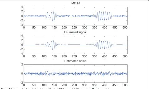
If mode mixing is present in the first IMF (d1[n]), it
becomes necessary to distinguish between the part of its energy due to noise and the part due to the signal mixed in with the IMF. To do this, we simply consider here the first IMF to be a noisy signal. We therefore apply a wavelet filter,fwavelet, to separate the part due to
1. Test ifd1[n] is stationary, if yes go to (4)
2. Extract fromd1[n] the part that is noiseb[n] and
the part that is signals[n] by wavelet filtering (fwavelet
(x))
a.s[n] =fwavelet(d1[n])
b.b[n]= d1[n] -s[n]
3. Mode de-mixing a.d1[n] =b[n]
b.d2[n] =d2[n] +s[n]
4. Apply the classic algorithm for selecting IMFs as described in the previous section.
Every kind of wavelet filter could be used, e.g. discrete wavelet filter or wavelet packet filter. The choice depends on the characteristics of the signal of interest. In this work we chose to use a discrete wavelet filter, which is the simplest of all possible wavelet filters.
Evaluation of the new algorithm 1. Signals
In this work, we tested our algorithm on several kinds of signals: a purely synthetic signal made from three Gabor atoms, a signal generated by a vibrating ball bear-ing, and finally, an ECG signal generated using a model proposed by McSharry et al. [7]. We evaluated the robustness of our method by adding Gaussian white noise to these signals to obtain SNR values of 20, 18, 16, 14, and 12 dB. For each SNR, we studied 500 realizations.
2. IMF selection or denoising performances
We used, as an evaluation criterion, the normalized per-cent mean square error (NPMSE) between the original signal without noise and the reconstructed signal. NPMSE is defined as:
NPMSE = 100× n
i=1
x[i]− ˆx[i]2
n i=1x[i]2
(4)
wherexand xˆ are the original and the denoised sig-nal, respectively.
We compared the‘classic’ method (from [2]) to the improved approach proposed in this paper. We also compared the classic method to our approach, but with-out adding to the reconstruction the part of the first IMF corresponding to the signal (step 3b). In that way, we tested separately the effect of the cutoff values cor-rection, on the reconstruction of the signal.
We also studied the influence of the wavelet choice and of the number of decomposition levels (step 2a) on the performance of the new algorithm proposed. We tested the Daubechie of order 8, Meyer and Haar wave-lets and 5, 8, and 10 decomposition levels. In all experi-ments, the noise estimation in the decomposition levels was done using the heuristic variant of the Stein’s
unbiased rule. A soft threshold was then applied on each decomposition level before the reconstruction of the denoised original signal.
3. IMF characteristics
The IMFs and the residual signal from the first IMF are summed up after the application of the algorithm to reconstruct the signal. In the de-mixing step of the pro-posed algorithm, we chose to add the part of the signal extracted from the first IMF to the second IMF. This addition of a part of the first IMF to the second can make the second IMF lose some of its characteristics as a true IMF. Although this does not affect the process of signal reconstruction and does not diminish the quality of the reconstructed signal, it may be important to pre-serve the characteristics of the EMD decomposition, if further processing of the signal is to be done. As an example we may be interested in the Hilbert-Huang spectrum of the different IMFs.
To clarify the issue of how much our algorithms have induced the second IMF to differ from a true IMF, we created a method to quantify how close the modified IMF is to a true IMF.
If a signal (s(t)) has all the properties of an IMF, its EMD will result in one and only one IMF that will be identical to the signal itself. In this case, the first IMF’s energy relative to the signal will be 100%. If the analyzed signal is not a pure IMF, its decomposition is going to result in several IMFs. Therefore, the energy of the first IMF, obtained from the signal, will be increasingly smal-ler as the signal is further away from being a pure IMF.
We therefore defined an ‘IMF-likeness’ measure to quantify the modification to the second IMF. We first applied EMD to the IMFi(modified second IMF) to be
tested. Then, we computed the energy of the first IMF, obtained from this decomposition of IMFi, divided by its
original energy (energy of IMFi). If IMFi still has the
characteristics of an IMF, this ratio gives a number close to 1, but gives a smaller value when IMFi is less
like an IMF.
Results
Figure 1 shows an example of the EMD obtained on a synthetic signal composed of three Gabor atoms with 12 dB noise added. We can clearly see that the first IMF contains mode mixing. Indeed, a part of the signal is clearly evident in this mode. The energy of the IMF that corresponds to the signal is stronger than the noise energy. It will, therefore, lead to an over-estimation of the noise contained in the original signal.
Figure 2 presents the estimation of the noise model and the associated confidence interval (TH) by means of
si
gn
al
Empirical Mode Decomposition
im
f1
im
f2
im
f3
im
f4
im
f5
im
f6
im
f7
res
.
Figure 1EMD of a synthetic signal with 12 dB SNR.
0 1 2 3 4 5 6 7 8
-15 -10 -5 0
lo
g 2
(en
er
gy
)
0 1 2 3 4 5 6 7 8
-15 -10 -5 0
IMF
lo
g 2
(en
er
gy
)
Model T
H
Model T
H
Figure 2 An example of the selection of modes of the signal presented in Figure 1 by the classic algorithm (above) and by the
method presented in this work (below). The estimated model and the associated confidence interval (TH) are presented as a straight line and
that the over-estimation of the noise level leads to the rejection of IMFs 4 to 6, even though they clearly con-tain a part of the original signal. To correct this, if we detect the presence of mode mixing in the first IMF, we propose, in the new algorithm, to separate the part cor-responding to the signal from that corcor-responding to noise. Figure 3 presents the mode de-mixing result obtained by our algorithm. The correction of the noise level estimation results in the appropriate selection of IMFs 4 to 6 (Figure 2, lower panel).
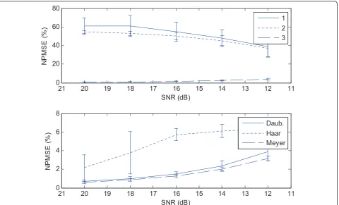
Figure 4 presents the results of the robustness analysis for the three algorithms tested: the classical method (1), the de-mixing of IMF1 only (2), the de-mixing plus addition of the IMF1 signal to IMF2 (3). Correcting the noise level estimation in IMF1 (method 2) induces a reduction of the reconstruction error when compared to method 1 (Figure 4, upper panel). In addition, if the sig-nal contained in the IMF1 is taken into account in IMF2, the level of reconstruction error drops to very small values, for all values of SNR. In all cases, the results of our method are better than those obtained with the classical method. We also note that the stan-dard deviation is smaller for our methods in all cases.
Figure 4 (lower panel) presents the influence of the choice of wavelet. We can notice that the different wavelets influence the quality of the results. In particu-lar, Haar’s wavelet provides the worst results. Meyer’s
and Daubechie’s wavelets give similar results even if the error is slightly lower for Meyer’s wavelet. The error obtained using either of these two wavelets is lower than 5%. The number of levels of the wavelet decompo-sition had a negligible effect on the quality of the recon-struction (results not shown). This can be explained by the relatively great difference in the frequency content of the signal and of the noise contained in the first IMF of the synthetic signal under study.
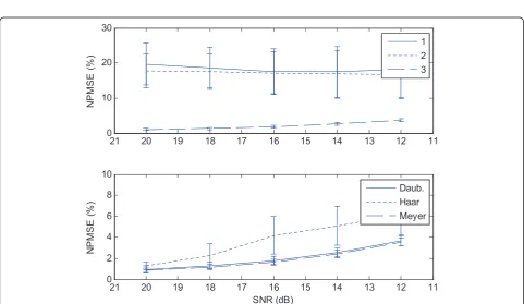
When applied to the ball bearing signal (Figure 5) or to the simulated ECG signals (Figure 6), the results of the algorithms are similar to those obtained for the syn-thetic signal. The standard deviations are, however, greater for the ECG signals than those obtained on the other signals. This is most probably due to the high variability of the number of QRS complexes contained in the first IMF in different realizations of the noisy sig-nal. For these signals, the number of levels of the wave-let decomposition also has a very small effect on the reconstruction error, even though the effect is higher than the one observed for synthetic signals.
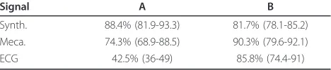
Table 1 presents the results obtained for the ‘IMF likeness measure’ for the different signals used in this study, with a 16 dB SNR. We can generally notice that the signal obtained by removing the noise from the first IMF (first denoised IMF) is not an IMF according to our measure (Table 1, column A). It is, however, fairly
0 50 100 150 200 250 300 350 400 450 500
-4 -2 0 2 4
IMF #1
0 50 100 150 200 250 300 350 400 450 500
-4 -2 0 2 4
Estimated signal
0 50 100 150 200 250 300 350 400 450 500
-2 0
2 Estimated noise
close to being an IMF except for the case of the ECG signals. For the mechanical (ball bearing) and ECG sig-nals, adding the signal part of the first IMF (first denoised IMF) to the second IMF gives better IMF-like characteristics, according to our measure (Table 1, col-umn B). Only for the synthetic signals, this addition reduces the IMF likeness measure.
Conclusion
We have proposed in this paper an improvement of an existing algorithm used for selecting the IMFs of inter-est, which is useful in case of mode mixing that can affect the performances of the original algorithm. The existing algorithm uses the first IMF to provide an esti-mate of the noise contained in each of the IMFs of an EMD. The presence of a mixing of modes introduces errors to this estimation and may lead to a bad selection of the IMFs of interest. Our approach is based on the detection of mode mixing by a test of stationarity on the first IMF, and on the extraction of the part of the first IMF that corresponds to pure noise. The choice of the stationarity test and of the noise extraction algo-rithm has to be made according to the specific signal of interest. In this work, we chose a stationarity test based
on the statistical study of time-frequency surrogates of the signal, and a wavelet filter for separating noise from signal in the first IMF. These choices present the advan-tage of not making a priori assumptions about the sig-nals under study. The only strong hypothesis is that the corrupting noise is stationary and stays stationary during the decomposition process by EMD. We have shown improved results with respect to the algorithm for sig-nals having very different characteristics. We have demonstrated that our algorithm is robust with respect to noise for all of the studied signals. A de-mixing step is used in the algorithm. We have shown, specifically for the synthetic signals, that this step may not lead to an improvement, depending on the application, i.e. depend-ing on whether the signal is simply to be reconstructed or if a further analysis of the individual IMFs using Hil-bert spectrum is the objective of the processing. The evaluation of the proposed IMF likeness measure could indicate if this step is suitable for a further spectral ana-lysis. If the measure obtained on the first denoised IMF is higher than the one obtained on the sum of this first denoised IMF and the second one, we would suggest not doing the step 3b. In this case, it is more suitable to add a new IMF corresponding to the first denoised one,
11 12 13 14 15 16 17 18 19 20 21 0 20 40 60 80
SNR (dB)
NP
M
S
E
(%
)
1 2 3
11 12 13 14 15 16 17 18 19 20 21 0 2 4 6 8
SNR (dB)
NP
M
S
E
(
%
)
Daub. Haar Meyer
11 12 13 14 15 16 17 18 19 20 21 0 5 10 15 20 25
NP
M
S
E
(%
)
1 2 3
11 12 13 14 15 16 17 18 19 20 21 0 2 4 6 8 10
SNR (dB)
NP
M
S
E
(%
)
Daub. Haar Meyer
Figure 5Results on the mechanical signal from the ball bearing plus noise. Above: The evolution of the percentage of mean square error (NPMSE) (±s) as obtained by using the classic method (1), by only correcting the estimate of noise in the first IMF (2) and by correcting the estimate of noise in the first IMF and plus modification of the second IMF (3). Below: Comparison of the NPMSE obtained using the wavelets Daubechie (Daub.), Haar and Meyer.
11 12 13 14 15 16 17 18 19 20 21 0 10 20 30
NP
M
S
E
(%
)
1 2 3
11 12 13 14 15 16 17 18 19 20 21 0 2 4 6 8 10
SNR (dB)
NP
M
S
E
(%
)
Daub. Haar Meyer
before computing the Hilbert-Huang spectrum of the signal of interest. A deeper analysis of the reasons of these losses of IMF characteristics may help to define more efficient strategies in order to further improve the spectral estimation of the signals of interest.
List of abbreviations
EMD: empirical mode decomposition; IMF: intrinsic mode functions.
Acknowledgements
This work was supported by the Icelandic center for the research «RANNIS».
Author details 1
Department of electronics, Université de Technologie de Compiègne, Compiègne Cedex, F60205, France2UMR CNRS 6600, Université de Technologie de Compiègne, Compiègne Cedex, F60205, France3School of Science and Engineering, Reykjavik University, Menntavegur 1, Reykjavik 103, Iceland
Competing interests
The authors declare that they have no competing interests.
Received: 10 December 2010 Accepted: 8 August 2011 Published: 8 August 2011
References
1. NE Huang, Z Shen, SR Long, MC Wu, HH Shih, O Zheng, N Yen, CC Tung, HH Liu, The empirical mode decomposition and the hilbert spectrum for nonlinear and non-stationary time series analysis. Proc R Soc Math Phys Eng Sci.454, 903–995 (1998). doi:10.1098/rspa.1998.0193
2. Z Wu, NE Huang, A study of the characteristics of white noise using the empirical mode decomposition method. Proc R Soc Math Phys Eng Sci. 460, 1597–1611 (2004). doi:10.1098/rspa.2003.1221
3. P Flandrin, P Goncalves, G Rilling, inEMD Equivalent Filter Banks, from Interpretation to Applications, ed. by NE Huang, SSP Shen Hilbert-Huang Transform and Its Applications (World Scientific, Singapore, 2005), pp. 57–74 4. R Deering, JF Kaiser, The use of a masking signal to improve empirical
mode decomposition. inIEEE International Conference on Acoustics, Speech, and Signal Proceedings, Philadelphia, PA, USA, (2005)
5. M Blanco-Velasco, B Weng, KE Barner, ECG signal denoising and baseline wander correction based on the empirical mode decomposition. Comput Biol Med.38, 1–13 (2008). doi:10.1016/j.compbiomed.2007.06.003 6. J Xiao, P Borgnat, P Flandrin, Testing stationarity with time-frequency
surrogates. inXVth European Signal Proceedings Conference, Poznan, Poland, (2007)
7. PE McSharry, GD Clifford, L Tarassenko, LA Smith, A dynamical model for generating synthetic electrocardiogram signals. IEEE Trans Biomed Eng.50, 289–294 (2003). doi:10.1109/TBME.2003.808805
doi:10.1186/1687-6180-2011-37
Cite this article as:Terrienet al.:Automatic detection of mode mixing in empirical mode decomposition using non-stationarity detection:
application to selecting IMFs of interest and denoising.EURASIP Journal
on Advances in Signal Processing20112011:37.
Submit your manuscript to a
journal and benefi t from:
7Convenient online submission 7Rigorous peer review
7Immediate publication on acceptance 7Open access: articles freely available online 7High visibility within the fi eld
7Retaining the copyright to your article
Submit your next manuscript at 7 springeropen.com Table 1 Median of the relative energy (lower
quartile-upper quartile), expressed as a percentage of the first IMF obtained after EMD of the: first denoised IMF (A), second IMF + first denoised IMF (B)
Signal A B
Synth. 88.4% (81.9-93.3) 81.7% (78.1-85.2)
Meca. 74.3% (68.9-88.5) 90.3% (79.6-92.1)
ECG 42.5% (36-49) 85.8% (74.4-91)