Compressed Sensing, Sparse Approximation, and Low-Rank Matrix Estimation

(1)

Compressed sensing, sparse approximation, and low-rank

matrix estimation

Thesis by

Yaniv Plan

In Partial Fulfillment of the Requirements for the Degree of

Doctor of Philosophy

California Institute of Technology Pasadena, California

2011

(2)

(3)

(4)

Abstract

The importance of sparse signal structures has been recognized in a plethora of applications ranging from medical imaging to group disease testing to radar technology. It has been shown in practice that various signals of interest may be (approximately) sparsely modeled, and that sparse modeling is often beneficial, or even indispensable to signal recovery. Alongside an increase in applications, a rich theory of sparse and compressible signal recovery has recently been developed under the names compressed sensing (CS) and sparse approximation (SA). This revolutionary research has demon-strated that many signals can be recovered from severely undersampled measurements by taking advantage of their inherent low-dimensional structure. More recently, an offshoot of CS and SA has been a focus of research on other low-dimensional signal structures such as matrices of low rank. Low-rank matrix recovery (LRMR) is demonstrating a rapidly growing array of important appli-cations such as quantum state tomography, triangulation from incomplete distance measurements, recommender systems (e.g., the Netflix problem), and system identification and control.

In this dissertation, we examine CS, SA, and LRMR from a theoretical perspective. We consider a variety of different measurement and signal models, both random and deterministic, and mainly ask two questions.

How many measurements are necessary? How large is the recovery error?

(5)

Acknowledgements

I am very grateful for the intelligent way in which my advisor, Emmanuel Cand`es, stoked my interest first in the classes that I took from him and later through years of research. His intuitive view of the material and his emphasis on tackling important (and difficult) problems was ideal for me. His ability to identify such research problems and ask substantial questions about them made it much easier for me to produce as a graduate student. I also appreciate the many mathematical concepts he has taught me, and exposed me to, and the resources he has shown me to help me learn material on my own.

Aside from my advisor, I would like to thank several fellow graduate students and postdocs for their help and support, both in working through math problems and also for giving me advice on my writing. In particular, thanks to Stephen Becker, Alex Gittens, Ewout Vandenberg, Deanna Needell, and Mark Davenport.

Throughout my stay at Caltech, Sheila Schull and Sydney Garstang did a wonderful job in providing information and help. It is amazing how much easier daily work is with them around.

I would like to thank Joel Tropp, Houman Owhadi, and Babak Hassibi for attending my thesis defense. Also, thanks to Joel and Houman for the material you have taught me in class—it is quite clear that you care about teaching well, and the benefits of this care are evident in the classroom. In fact, as I hope to lecture classes myself in the near future, I plan to incorporate some of the teaching techniques that I learned from watching you two (and from Emmanuel as well).

(6)

List of Tables

(11)

List of Figures

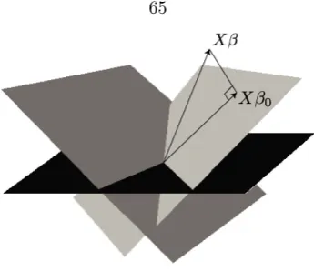
3.1 The vector Xβ0 is the projection of Xβ on an ideally selected subset of covariates. These

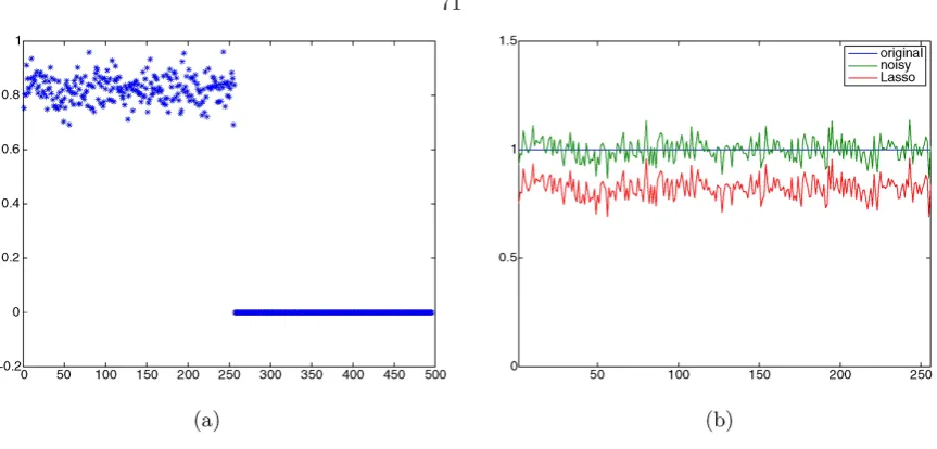
covariates span a plane of optimal dimension which, among all planes spanned by subsets of the same dimension, is closest toXβ. . . 65 3.2 Sparse signal recovery with the LASSO. (a) Values of the estimated coefficients. All the spike

coefficients are obtained by soft-thresholdingyand are nonzero. (b) LASSO signal estimate;

Xβˆis just a shifted version of the noisy signal. . . 71

(12)

Chapter 1

Introduction

An image of blood vessels in the body, which may be captured through MRI, has an abundance of structure; in particular, it is sparse in space, and its spatial finite differences are even sparser. Can this structure be utilized to improve MR imaging? Resoundingly, yes! In fact, by taking into account sparsity, MR imaging can be (and has been) sped up by a factor of 7, as demonstrated through a double blind study [159]. The improvement applies outside of just angiography, to MR images in general, which tend to be sparse in the appropriate basis. Moreover, the benefits can be life altering in cases when a slow MR scan is not feasible [71]. The research that has lead to these improvements is called compressed sensing and is closely related to sparse approximation. CS was born seven years ago, pioneered by the papers [39, 42, 55], and it is still being intensely researched today.

1.0.1

Compressed sensing

In CS, a signal x∈ Cn is modeled as a superposition of a small number of elements from a given dictionary, Φ∈Cn×k_{. In other words,} _x=_Φ_v_{, where}_v∈Ck _{is sparse (it has few nonzero elements).}

The basic goal is to recover an approximation ofxfrom linear measurements corrupted by noise

y=Ax+z (1.0.1)

whereA∈Cm×n _{is a measurement matrix (often constructed by the scientist), and}_z_{is a noise term.} For example, in MRI Φ may be a wavelet dictionary, andAcan be modeled as a subsampling of the rows of a descrete fourier transform (DFT).

An interesting point about the theory of CS is that it generally requires random measurements (e.g., A could be a random subsampling of the DFT). Not only is this assumption crucial to the derivation of many strong theoretical results, but also random measurements seem to give better results in practice and are sought out in real applications.

(13)

it to be the identity), so thatxitself should be sparse.1 _{With this simplification CS is a special case} of a more general class of problems called SA.

1.0.2

Sparse approximation

Once again in SA, we would like to recover a sparse vectorxfrom linear measurementsy=Ax+z, but there is still one subtle difference between CS and SA. Whereas in CS A is a measurement matrix which in most applications may be constructed (randomly) by the scientist (e.g., in MRI, one chooses which Fourier coefficients to sample), in SA in general there is no expectation that the structure of Amay be affected by the scientist. Ais often a deterministic, unalterable matrix, and this leads to different theoretical aspects of the problem and a quite different analysis. As an example of SA, in statistical model selection, Ais the design matrix, filled with response variables (e.g., answers to a survey). Sparsity plays an important role because often only a few regressors (columns of A) are significant. (Statisticians will be more familiar with the notation y =Xβ+z,

X∈Rn×p_.)

While MRI and the statistical linear model are important examples, sparse signal structures are ubiquitous throughout science and engineering (and we will point to several more examples throughout the thesis). They often arise from the parsimonious nature of the signal—often the underlying structure depends on just a few parameters. In some cases this leads to sparse signals, or, in another vein, this may lead to matrix-valued signals with low rank; this is the second signal structure considered in this thesis.

1.0.3

Low-rank matrix recovery

As a quintessential example of LRMR, consider the semi-famous Netflix problem, in which one has available several entries of the Netflix movie-rating matrix. This matrix contains at position i, j

the rating (or estimated rating) of user ifor moviej. The goal is to fill in the missing entries—in particular, Netflix would like to be able to predict user ratings for unrated movies. Now, it turns out that the Netflix matrix is (approximately) low-rank; the theoretical justification for this phenomena is that there are only a few important factors which effect peoples’ movie ratings. For example, a few ostensible factors would be the user’s predilection towards drama, comedy, and violence. However, due to the general methods used for LRMR (see Chapter 4), it is completely unnecessary to know exactly which factors contribute—these are discovered along with the missing entries.

The Netflix problem is an example of a subclass of LRMR problems called matrix completion. However, LRMR, has many applications (see Chapters 4 and 5), which follow from a more general

1_{This is fairly innocuous for unitary transforms, since they are isometries in the}_`

2 norm. For a treatment of CS

(14)

model:

y= A(M) +z

wherey is a vector of noisy measurements,A ∶Rn1×n2 →_m_{is a linear measurement operator,}_z _{is a}

noise term, andM ∈Rn1×n2 _{is a matrix with low rank. The goal is to recover}_M_.

1.0.4

Peek at the results

In this thesis we study the effectiveness of convex optimization to recover sparse vectors and low-rank matrices from noisy, linear measurements. In fact, beyond estimatingxfrom equation (1.0.1), we also consider the accurate recovery ofAxand the support of x. The theory will show that one may take far fewer samples than the ambient dimension of the signal; instead the number of samples must match (approximately) the number of dimensions of the manifold that the signal resides in. For example, vectors of length nwith sparsity level exactly slie in an sdimensional manifold; in Chapters 2 and 3 we show that in many cases on the order of slognmeasurements are sufficient for stable recovery by `1-minimization-based programs. Similarly, rank(r), n×n matrices lie in a manifold with dimension 2nr−r2_{; in Chapters 4 and 5 we show that they may be stably recovered} by nuclear-norm-minimization-based programs from approximately nr, or nrlog2n, measurements (depending on the measurement model).

While the manifolds that our signals lie in are quite nonlinear, they contain many linear subspaces with (approximately) the same dimension as the original manifolds. In Chapters 3 and 4, this is used to develop lower bounds on the error achievable by any recovery method. We consider an oracle which gives away the smaller linear subspace that the signal resides in; from this point it is easy to analyze the error achieved by least squares regression (which is minimax). As is well known, in the case of Gaussian noise, this leads to an error proportional to the dimension of the linear subspace, and thus proportional to the dimension of the underlying manifold. Interestingly, we give upper bounds for the error achieved by convex optimization, which nearly match these lower bounds. In other words, by taking into account the parsimony of the model, the error in estimation is not proportional to the entire noise vector, but rather to the norm of the noise vector projected onto a much smaller subspace.

1.0.5

The restricted isometry property

A quite prevalent way to prove results about the efficacy of `1 minimization, nuclear-norm mini-mization, and a large array of other recovery techniques is the use of the RIP. From here on, we call a vectors-sparse if it has at most snonzero entries.

(15)

RIP with parameterssandδ if

(1−δ)∥v∥2`2≤ ∥Av∥

2

`2 ≤ (1+δ)∥v∥

2

`2 (1.0.2)

for alls-sparse vectors v.

In other words, A should be well conditioned when acting on signals of interest. When the RIP holds with parameters 2s and δ < √2−1 [28] or even δ ≤ 0.453. . . [78], it is known that certain convex optimization programs are stable. In particular the LASSO and Dantzig selector, both`1 -minimization-based convex programs introduced in Chapter 2, accurately recover all signalsxwith at mostsnonzero elements.

An analogous version of the RIP holds for LRMR (see Chapter 4); in this case one asks the measurement operator A to be well conditioned when acting on low-rank matrices. As shown in Chapter 4, once again this demonstrates stability of convex optimization.

However, there are a number of limitations to RIP-based theory: 1) testing for the RIP is generally an intractable, combinatorial problem; 2) the only deterministic measurement ensembles which are known to satisfy the RIP do so only under extremely strong conditions; 3) the random measurement ensembles that satisfy the RIP (with high probability) are lacking in many applications; 4) the RIP provides uniform guarantees overall low-dimensional signals of interest, and thus theory with the RIP isnecessarily limited by worst-case signals (and similarly for other conditions which provide uniform guarantees such as the RIP-1 [81] and restricted strong convexity [116]). However, numerical experiments [58] and theoretical results (some of which are contained in this thesis) demonstrate that in many cases typical signals may be accurately recovered far past the point when worst-case signals are unrecoverable.

In fact, proving ‘RIP-less’ results is a delicate matter. To see the difficulty, note that to have universal results, i.e., results that hold for all sparsex(or low-rank M), simultaneously, the lower bound of the RIP would be a necessary condition for stability. To illustrate the point, take the case of SA, and suppose that an oracle gives the exact support,T, of the signalx. Then, one would need the pseudo inverse of AT (A restricted to the columns in T) to be bounded. In other words, the minimum singular value ofAT should be away from zero.

Thus, the RIP-less results in Chapters 2, 3, 5 are not universal, but rather they must take into account the structure of a typical signal. We do this in a variety of ways.

Fix the signal independent of the measurement ensemble (see Chapters 2 and 5):

(16)

Adopt a statistical model for the signal (see Chapter 3): Adopting a statistical model is a straightforward way to avoid worst-case signals, and can be used to prove results (with high probability) about general signals. This may be interpreted as proving results for most

signals of interest.

Assume extra signal structure (see Chapter 5): Here, we assume that the signal x

belongs to a certain (large) subset of its inherent low-dimensional space, and prove results given this assumption. (These assumptions are also calledincoherence assumptions in matrix completion.)

1.0.6

Organization

Each of the chapters, as described below, is self-contained, including notation. Also, they are all based upon research conducted jointly with my advisor, Emmanuel Cand`es.

Chapter 2: In this chapter, we introduce a simple and very general theory of CS. In this theory, the sensing mechanism simply selects sensing vectors independently at random from a probability distribution F; it includes all models—e.g. Gaussian, frequency measurements—discussed in the literature, but also provides a framework for new measurement strategies as well. We prove that if the probability distribution F obeys a simple incoherence property and an isotropy property, one can faithfully recover approximately sparse signals from a minimal number of noisy measurements. The novelty is that these recovery results do not require the restricted isometry property (RIP)—they make use of a much weaker notion—or a random model for the signal. As an example, in this chapter we show that a signal withsnonzero entries can be faithfully recovered from aboutslognFourier coefficients that are contaminated with noise.

Chapter 3: In this chapter, we turn to the sparse approximation problem which applies in partic-ular to model selection; thus we switch to the standard statistics notation. We first consider the fundamental problem of estimating the mean vector, Xβ, from the data y=Xβ+z. X is ann×pdesign matrix in which one can have far more variables than observations andz isz

is a mean-zero, stochastic error term—the so-called ‘p>n’ setup. Whenβ is sparse, or more generally, when there is a sparse subset of covariates providing a close approximation to the unknown mean vector, we ask whether or not it is possible to accurately estimateXβ using convex optimization.

(17)

logarithmic factor of the ideal mean squared error one would achieve with an oracle supplying perfect information about which variables should be included in the model and which variables should not. Interestingly, our results describe the average performance of the LASSO; that is, the performance one can expect in an vast majority of cases where Xβ is a sparse or nearly sparse superposition of variables, but not in all cases.

These results are widely applicable since they simply require that pairs of predictor variables are not too collinear.

Chapter 4: This chapter presents several novel theoretical results regarding the recovery of a low-rank matrix from just a few measurements consisting of linear combinations of the matrix entries. We show that properly constrained nuclear-norm minimization stably recovers a low-rank matrix from a constant number of noisy measurements per degree of freedom. Further, with high probability the recovery error from noisy data is within a constant of three targets: 1) the minimax risk, 2) an oracle error that would be available if the column space of the matrix were known, and 3) a more adaptive oracle error which would be available with the knowledge of the column space corresponding to the part of the matrix that stands above the noise. Lastly, the error bounds regarding low-rank matrices are extended to provide an error bound when the matrix has full rank with decaying singular values. The analysis in this chapter is based on the restricted isometry property.

Chapter 5: This chapter turns to the RIP-less matrix completion problem. We first survey the novel literature on matrix completion, which shows that under some suitable conditions, one can recover an unknown low-rank matrix from a nearly minimal set of entries by nuclear-norm minimization subject to data constraints. Further, this chapter introduces novel results showing that matrix completion is provably accurate even when the few observed entries are corrupted with a small amount of noise. A typical result is that one can recover an unknown

n×n matrix of low rank r from just about nrlog2n noisy samples with an error which is proportional to the noise level. We present numerical results which complement our quanti-tative analysis and show that, in practice, nuclear-norm minimization accurately fills in the many missing entries of large low-rank matrices from just a few noisy samples. Some analogies between matrix completion and compressed sensing are discussed throughout.

(18)

Chapter 2

A general model for CS

2.1

Introduction

This chapter develops a novel, simple, general, and ‘RIP-less’ theory of CS [39, 42, 55]. We begin by motivating and stating the results, and in turn give a discussion of related literature including a discussion of therestricted isometry property (RIP) in Section 2.1.7.

2.1.1

A RIP-less theory?

The early paper [39] triggered a massive amount of research by showing that it is possible to sample signals at a rate proportional to their information content rather than their bandwidth. For instance, in a discrete setting, this theory asserts that a digital signalx∈Rn _{(which can be viewed as Nyquist} samples of a continuous-time signal over a time window of interest) can be recovered from a small random sample of its Fourier coefficients provided that xis sufficiently sparse. Formally, suppose that our signalxhas at mosts nonzero amplitudes at completely unknown locations and that we are given the value of its discrete Fourier transform (DFT) atm frequencies selected uniformly at random (we think of m as being much smaller thann). Then [39] showed that one can recover x

by solving an optimization problem which simply finds, among all candidate signals, that with the minimum`1 norm; the number of samples we need must be on the order ofslogn. In other words, if we think of s as a measure of the information content, we can sample nonadaptively nearly at the information rate without information loss. By swapping time and frequency, this also says that signals occupying a very large bandwidth but with a sparse spectrum can be sampled (at random time locations) at a rate far below the Shannon-Nyquist rate.

Despite considerable progress in the field, some important questions have still been left open. We discuss two that have both a theoretical and practical appeal.

(19)

possible when these coefficients are further corrupted by noise?

These issues are paramount since in real-world applications, signals are never exactly sparse, and measurements are never perfect either. Now the traditional way of addressing these types of problems in the field is by means of the restricted isometry property (RIP) [41]. The trouble here is that it is unknown whether or not this property holds when the sample sizem is on the order of slogn. In fact, answering this one way or the other is generally regarded as extremely difficult, and so the restricted isometry machinery does not directly apply in this setting.

In this chapter, we prove that the two questions formulated above have positive answers. In fact, we introduce recovery results which are—up to a logarithmic factor—as good as those one would get if the restricted isometry property were known to be true. To fix ideas, suppose we observem

noisy discrete Fourier coefficients about ans-sparse signalx,

˜

yk= n−1

∑

t=0

e−ı2πωkt_x[_t] +_σz

k, k=1, . . . , m. (2.1.1)

Here, the frequencies ωk are chosen uniformly at random in{0,1/n,2/n, . . . ,(n−1)/n} and zk is white noise with unit variance. Then if the number of samples m is on the order of slogn, it is possible to get an estimate ˆxobeying

∥xˆ−x∥2_`₂=polylog(n) s mσ

2

(2.1.2)

by solving a convex`1-minimization program. (Note that when the noise vanishes, the recovery is exact.) Up to the logarithmic factor, which may sometimes be on the order of lognand at most a small power of this quantity, this is optimal. Now if the RIP held, one would get a squared error bounded by O(logn)_msσ2 [17, 43] and, therefore, the ‘RIP-less’ theory developed in this chapter roughly enjoys the same performance guarantees.

2.1.2

A general theory

The estimate we have just seen is not isolated and the real purpose of this chapter is to develop a theory of compressive sensing which is both as simple and as general as possible.

At the heart of compressive sensing is the idea that randomness can be used as an effective sensing mechanism. We note that random measurements are not only crucial in the derivation of many theoretical results, but also generally seem to give better empirical results as well. Therefore, we propose a mechanism whereby sensing vectors are independently sampled from a populationF. Mathematically, we observe

˜

yk= ⟨ak, x⟩ +σzk, k=1, . . . , m, (2.1.3)

where x∈ Rn, {zk} is a noise sequence, and the sensing vectors ak iid

(20)

family of complex sinusoids, this is the Fourier sampling model introduced earlier. All we require fromF is an isotropy property and an incoherence property.

Isotropy property: We say thatF obeys the isotropy property if

Eaa∗=_I_, _a∼_F. _(2.1.4)

IfF has mean zero (we do not require this), thenEaa∗ _{is the covariance matrix of}_F_{. In other}

words, the isotropy condition states that the components of a∼F have unit variance and are uncorrelated. This assumption may be weakened a little, as we shall see later.

Incoherence property: We may take the coherence parameterµ(F)to be the smallest number such that witha= (a[1], . . . , a[n]) ∼F,

max 1≤t≤n∣

a[t]∣2≤µ(F) (2.1.5)

holds either deterministically or stochastically in the sense discussed below. The smallerµ(F), i.e. the more incoherent the sensing vectors, the fewer samples we need for accurate recovery. When a simple deterministic bound is not available, one can take the smallest scalarµobeying

E[n−1_∥_a_∥2 `21Ec] ≤

1 20n

−3/2 _and _P₍_Ec_{) ≤ (}_nm₎−1_, _(2.1.6)

where Eis the event {max1≤t≤n∣a[t]∣2>µ}.

Suppose for instance that the components are i.i.d.N (0,1). Then a simple calculation we shall not detail shows that

E[n−1∥_a∥2

`21Ec] ≤2nP(Z> √µ) +2

√_µφ_(√_µ₎_, _(2.1.7)

P(Ec) ≤2nP(Z≥ √µ),

where Z is standard normal and φis its density function. The inequality P(Z >t) ≤φ(t)/t shows that one can take µ(F) ≤6 logn as long asn≥16 and m≤n. More generally, if the components of a are i.i.d. samples from a sub-Gaussian distribution, µ(F) is at most a constant times logn. If they are i.i.d. from a sub-exponential distribution, µ(F) is at most a constant times log2n. In what follows, however, it might be convenient for the reader to assume that the deterministic bound (2.1.5) holds.

(21)

DFT matrix as before, so that

a[t] =eı2πkt/n_,

where kis chosen uniformly at random in {0,1, . . . , n−1}. Then another simple calculation shows thatEaa∗=_I_and_µ(_F) =_{1 since}∣_a[_t]∣2=_{1 for all}_t_{. At the other extreme, suppose the measurement}

process reveals one entry ofxselected uniformly at random so thata=√n ei whereiis uniform in

{1, . . . , n}; the normalization ensures thatEaa∗=_I_{. This is a lousy acquisition protocol because one}

would need to sample on the order ofnlogntimes to recover even a 1-sparse vector (the logarithmic term comes from the coupon collector effect). Not surprisingly, this distribution is in fact highly coherent asµ(F) =n.

We pause to note that when specializing to subsampled Fourier measurements, this is a slightly different model that what has been considered in most past works [42, 135]. In particular, our model samples rows from a DFT with replacement, allowing the possibility of duplicates, whereas older works have considered sampling without replacement. These models are in fact essentially the same. First, when significantly undersampling, very few rows will be duplicated. Second, in the noiseless case, the only relevant facet ofAis its null space; sampling more rows decreases the null space and strictly aids in recovery. In particular, resampling a row provides no new information and does not decrease the null space. In other words, the probability that recovery fails when sampling mrows with replacement is strictly larger than than the probability that it fails when samplingmrows with replacement, i.e., our results extend to the other model. In the noisy case, the models appear to be quite similar, but neither is strictly weaker.

With the assumptions set, we now give a representative result of this chapter: suppose xis an arbitrary but fixeds-sparse vector and that one collects information about this signal by means of the random sensing mechanism (4.1.1), wherez is white noise. Then if the number of samples is on the orderµ(F)slogn, one can invoke`1minimization to get an estimator ˆxobeying

∥xˆ−x∥2_`₂≤polylog(n) s mσ

2

.

This bound is sharp. It is not possible to substantially reduce the number of measurements and get a similar bound, no matter how intractable the recovery method might be. To be precise, as shown in Section 2.1.5 the number of measurements required is sharp modulo a constant. Further, with this many measurements, the upper bound is optimal up to logarithmic factors. Finally, we will see that when the signal is not exactly sparse, we just need to add an approximation error to the upper bound.

(22)

2.1.3

Examples of incoherent measurements

We have seen through examples that sensing vectors with low coherence are global or spread out. Incoherence alone, however, is not a sufficient condition: ifF were a constant distribution (sampling fromFwould always return the same vector), one would not learn anything new about the signal by taking more samples regardless of the level of incoherence. However, as we will see, the incoherence and isotropy properties together guarantee that sparse vectors lie away from the nullspace of the sensing matrix whose rows are thea∗

k’s.

The role of the isotropy condition is to keep the measurement matrix from being rank defi-cient when suffidefi-ciently many measurements are taken (and similarly for subsets of columns of A). Specifically, one would hope to be able to recover any signal from an arbitrarily large number of measurements. However, if Eaa∗ _{were rank deficient, there would be signals} _x ∈ Rn _{that would}

not be recoverable from an arbitrary number of samples; just take x≠0 in the nullspace of Eaa∗_.

The nonnegative random variablex∗_aa∗_x_{has vanishing expectation, which implies}_a∗_x=_{0 almost}

surely. (Put differently, all of the measurements would be zero almost surely.) In contrast, the isotropy condition implies that _m1 ∑mk=1aka

∗

k → I almost surely as m → ∞ and, therefore, with enough measurements, the sensing matrix is well conditioned and has a left-inverse.1

We now provide examples of incoherent and isotropic measurements.

Sensing vectors with independent components. Suppose the components of a ∼ F

are independently distributed with mean zero and unit variance. Then F is isotropic. In addition, if the distribution of each component is light-tailed, then the measurements are clearly incoherent.

A special case concerns the case where a∼N(0,I), also known in the field as the Gaussian measurement ensemble, which is perhaps the most commonly studied. Here, one can take

µ(F) =6 lognas seen before.

Another special case is thebinary measurement ensemblewhere the entries ofaare symmetric Bernoulli variables taking on the values±1. A shifted version of this distribution is the sensing mechanism underlying the single pixel camera [68].

Subsampled orthogonal transforms: Suppose we have an orthogonal matrix obeying

U∗_U = _n_I_{. Then consider the sampling mechanism picking rows of} _U _{uniformly and}

inde-pendently at random. In the case where U is the DFT, this is the random frequency model introduced earlier. Clearly, this distribution is isotropic andµ(F) =maxij∣Uij∣2. In the case where U is a Hadamard matrix, or a complex Fourier matrix,µ(F) =1.

1_{One could require ‘near isotropy,’ i.e.,}_E_aa∗

≈I. If the approximation were tight enough, our theoretical results

(23)

Random convolutions: Consider the circular convolution modely=Gxin which

G= ⎡⎢ ⎢⎢ ⎢⎢ ⎢⎢ ⎢⎢ ⎢⎢ ⎢⎢ ⎢⎢ ⎣

g[0] g[1] g[2] . . . g[n−1]

g[n−1] g[0] g[1] . . .

g[1] . . . g[n−1] g[0]

⎤⎥ ⎥⎥ ⎥⎥ ⎥⎥ ⎥⎥ ⎥⎥ ⎥⎥ ⎥⎥ ⎦ .

Because a convolution is diagonal in the Fourier domain (we just multiply the Fourier compo-nents ofxwith those ofg),Gis an isometry if the Fourier components ofg= (g[0], . . . , g[n−1]) have the same magnitude. In this case, sampling a convolution product at randomly se-lected time locations is an isotropic and incoherent process provided g is spread out (µ(F) =

maxt∣g(t)∣2). This example extends to higher dimensions; e.g. to spatial 3D convolutions.

Subsampled tight or continuous frames: We can generalize the example above by sub-sampling a tight frame or even a continuous frame. An important example might be the Fourier transform with a continuous frequency spectrum. Here,

a(t) =eı2πωt,

where ω is chosen uniformly at random in [0,1] (instead of being on an equispaced lattice as before). This distribution is isotropic and obeys µ(F) =1. A situation where this arises is in magnetic resonance imaging (MRI) as frequency samples rarely fall on an equispaced Nyquist grid. By swapping time and frequency, this is equivalent to sampling a nearly sparse trigonometric polynomial at randomly selected time points in the unit interval [125].

These examples could of course be multiplied, and we hope we have made clear that our framework is general and encompasses many of the measurement models discussed in compressive sensing—and perhaps many new ones as well.

(24)

2.1.4

Matrix notation

Before continuing, we pause to demonstrate exactly how we display this model in the matrix notation of the introduction. Divide both sides of (4.1.1) by√m, and rewrite our statistical model as

y=Ax+σmz; (2.1.8)

thekth entry ofy is ˜yk divided by√m, thekth row ofAisa∗k divided by

√_m_{, and}_σ

misσdivided by√m. This normalization implies that the columns of Aare approximately unit-normed, and is most used in the compressive sensing literature.

2.1.5

Incoherent sampling theorem

To ease readability, we introduce our results by first presenting a recovery result from noiseless data. The recovered signal is obtained by the standard`1-minimization program

min ¯ x∈Rn ∥

¯

x∥`1 subject to A¯x=y. (2.1.9)

(Recall that the rows ofAare normalized independent samples fromF.)

Theorem 2.1.1 (Noiseless incoherent sampling) Let x be a fixed but otherwise arbitrary s -sparse vector inRn. Then with probability at least1−5/n−e−β_,_x_{is the unique minimizer to} _(2.1.9)

withy=Axprovided that

m≥Cβ⋅µ(F) ⋅s⋅logn.

More precisely, Cβ may be chosen asC0(1+β)for some positive numerical constant C0.

Among other things, this theorem states that one can perfectly recover an arbitrary sparse signal from aboutslognconvolution samples, or a signal that happens to be sparse in the wavelet domain from about slogn randomly selected noiselet coefficients. It extends an earlier result [38], which assumed a subsampled orthogonal model, and strengthens it since that reference could only prove the claim for randomly signed vectorsx. Here,xis arbitrary, and we do not make any distributional assumption about its support or its sign pattern.

This theorem is also about a fundamental information theoretic limit: the number of samples for perfect recovery has to be on the order ofµ(F) ⋅s⋅logn, and cannot possibly be much below this number. More precisely, suppose we are given a distributionF with coherence parameterµ(F). Then there exists-sparse vectors that cannot be recovered with probability at least 1−1/n, say, from fewer than a constant timesµ(F)⋅s⋅lognsamples. Whenµ(F) =1, this has been already established since [39] proves that some ssparse signals cannot be recovered from fewer than a constant times

(25)

Assume, without loss of generality, thatµ(F)is an integer and consider the isotropic process that samples rows from ann×nblock diagonal matrix, each block being a DFT of a smaller size; that is, of sizen/`whereµ(F) =`. Then ifm≤c0⋅µ(F) ⋅s⋅logn, one can constructs-sparse signals just as in [39] for whichAx=0 with probability at least 1/n. We omit the details.

The important aspect, here, is the role played by the coherence parameterµ(F). In general, the minimal number of samples must be on the order of the coherence times the sparsity levelstimes a logarithmic factor. Put differently,the coherence completely determines the minimal sampling rate.

2.1.6

Main results

We assume for simplicity that we are undersampling so thatm≤n. Our general result deals with 1) arbitrary signals which are not necessarily sparse (images are never exactly sparse even in a transformed domain) and 2) noise. To recoverxfrom the datay and the model (2.1.8), we consider the unconstrained LASSO [147] which solves the`1 regularized least-squares problem

min ¯ x∈Rn

1

2∥Ax¯−y∥ 2

`2+λσm∥x¯∥`1. (2.1.10)

We assume thatzis Gaussianz∼N(0,I). However, the theorem below may be adapted to any noise model that obeys ∥A∗_z∥

`∞ ≤C

√_log_n _{with high probability (for a fixed constant}_C_{). Thus many}

other noise models would work as well. In what follows,xsis the bests-sparse approximation ofx or, equivalently, a vector consisting of theslargest entries ofxin magnitude. Ties may be resolved in any arbitrary way.

Theorem 2.1.2 Letxbe an arbitrary fixed vector inRn_{. Then with probability at least}₁₋₆_/_n₋₆_e−β

the solution to (2.1.10)with λ=10√logn obeys

∥xˆ−x∥`2≤ min

1≤s≤s¯C(1+α)

⎡⎢ ⎢⎢ ⎢⎣

∥x−√xs∥`1

s +σ

√ slogn

m ⎤⎥ ⎥⎥

⎥⎦ (2.1.11)

provided that m≥Cβ⋅µ(F) ⋅s¯⋅logn. If one measures the error in the`1 norm, then

∥xˆ−x∥`1≤₁min

≤s≤¯s

C(1+α)⎡⎢⎢⎢

⎢⎣∥x−xs∥`1+sσ

√

logn m

⎤⎥ ⎥⎥

⎥⎦. (2.1.12)

Above, C is a numerical constant, Cβ can be chosen as before, and α=

√

(1+β)sµlognlogmlog2₍_sµ₎

m which is never greater thanlog3/2

n in this setup.

(26)

not necessarily imply uniform sparse-signal recovery, but instead they imply recovery of an arbitrary

fixed sparse signal with high probability. Further, the error bound is within at most a log3/2

nfactor of what has been established using the RIP since a variation on the arguments in [43] would give an error bound proportional to the quantity inside the square brackets in (2.1.11). As a consequence, the error bound is within a polylogarithmic factor of what is achievable with the help of an oracle that would reveal the locations of the significant coordinates of the unknown signal [43]. In other words, it cannot be substantially improved.

Because much of the compressive sensing literature works with restricted isometry conditions— we shall discuss exceptions such as [14,62] in Section 2.1.7—we pause here to discuss these conditions and to compare them to our own. As mentioned in Chapter 1, we say that anm×nmatrixAobeys the RIP with parameterssandδif

(1−δ)∥v∥2`2≤ ∥Av∥

2

`2 ≤ (1+δ)∥v∥

2

`2 (2.1.13)

for alls-sparse vectorsv. In other words, all the submatrices ofAwith at mostscolumns are well conditioned. When the RIP holds with parameters 2sandδ<0.414. . .[28] or evenδ≤0.453. . .[78], it is known that the error bound (2.1.11) holds (without the factor (1+α)). This δ is sometimes referred to as the restricted isometry constant.

Bounds on the restricted isometry constant have been established in [42] and in [135] for partial DFT matrices, and by extension, for partial subsampled orthogonal transforms. For instance, [135] proves that if A is a properly normalized partial DFT matrix, then the RIP with δ = 1/4 holds with high probability if m≥ C⋅slognlogmlog2s (C is some positive constant). We believe the proof extends with hardly any change to show that the measurement ensembles considered in this chapter obey the RIP with high probability when m ≥C⋅µ(F) ⋅slognlogmlog2(sµ). Thus, our result bridges the gap between the region where the RIP holds and the region in which one has the minimum number of measurements needed to prove perfect recovery of exactly sparse signals from noisy data, which is on the order ofµ(F) ⋅slogn. In doing so, we introduce an extra factorαinto our error bounds, which does not exist in the RIP-based results. This factor is at most logarithmic (α<log3/2

n) and shrinks with the number of measurements; when the RIP is known to hold, the factorαdisappears, i.e., α=O(1). With that said, we believe that in the region in which the RIP does not hold, andα>1, this extra factor is an artifact of the proof technique and could be removed by a different theoretical analysis. Last, we note that in certain regimes there are prior RIPless results that give stability guarantees whenm>Csµlogmlog5(µlogm)(see Section 3.1.2).

(27)

measurement ensemble). This slight loss is a small price to pay for a very simple general theory, which accommodates a wide array of sensing strategies. Having said this, the reader will also verify that specializing our proofs below gives an optimal result for the Gaussian ensemble; i.e. establishes a near-optimal error bound from aboutslog(n/s)observations.

Finally, another frequently discussed algorithm for sparse regression is the Dantzig selector [43]. Here, the estimator is given by the solution to the linear program

min ¯ x∈Rn ∥

¯

x∥`1 subject to ∥A

∗(_A_x_¯−_y)∥

`∞≤λ σm. (2.1.14)

We show that the Dantzig selector obeys nearly the same error bound.

Theorem 2.1.3 The Dantzig selector, withλ=10√lognand everything else the same as in Theo-rem 2.1.2, obeys

∥xˆ−x∥`2≤min_s

≤¯s

C(1+α2)⎡⎢⎢⎢ ⎢⎣

∥x−√xs∥`1

s +σ

√ slogn

m ⎤⎥ ⎥⎥

⎥⎦ (2.1.15)

∥xˆ−x∥`1≤min_s

≤¯s

C(1+α2)⎡⎢⎢⎢

⎢⎣∥x−xs∥`1+sσ

√

logn m

⎤⎥ ⎥⎥

⎥⎦ (2.1.16)

with the same probabilities as before.

The only difference isα2 _{instead of}_α_{in the right-hand sides.}

2.1.7

Our contribution

Due to the plethora of background literature, we reverse the standard order and first describe our contribution before describing many of the important contributions that came before it, in Section 3.1.2.

(28)

that the restricted isometry property is not necessarily needed to accurately recover nearly sparse vectors from noisy compressive samples. Thus our work is a significant departure from the majority of the literature, which establishes good noisy recovery properties via the RIP machinery. This literature is, of course, extremely large and we cannot cite all contributions but a partial list would include [9, 10, 17, 26, 40, 42, 43, 51, 56, 94, 124, 135, 166, 167].

The reason why one can get strong error bounds, which are within a polylogarithmic factor of what is available with the aid of an ‘oracle’, without the RIP is that our results do not imply universality. That is, we are not claiming that ifAis randomly sampled and then fixed once for all, then the error bounds from Section 2.1.6 hold for all signals x. What we are saying is that if we are given an arbitrary x, and then collect data by applying our random scheme, then the recovery of this xwill be accurate. As discussed in Chapter 1, if one wishes to establish universal results holding forall xsimultaneously, then we would need the RIP or a property very close to it. As a consequence, we cannot possibly be in this setup and guarantee universality since we are not willing to assume that the RIP holds.

To the best of our knowledge, only a few papers have addressed non-universal stability (the literature grows so rapidly that an inadvertent omission is entirely possible). In Chapter 3 we also consider weak conditions that allow stable recovery; in this case the we assume that the signal is sampled according to a random model, but in return the measurement matrixAcan be deterministic. In the asymptotic case, stable signal recovery has been demonstrated for the Gaussian measurement ensemble in a regime in which the RIP does not necessarily hold [14,62]; these papers will be discussed more below, and in the asymptotic limit they provide exact answers. This contrasts with our non-asymptotic theory which non-exact, but gives bounds that are tight to within logarithmic factors. Aside from these papers and the work in progress [35], it seems that that the literature regarding stable recovery with conditions weak enough that they do not imply universality is extremely sparse. Finally and to be complete, we would like to mention that earlier works have considered the recovery of perfectly sparse signals from subsampled orthogonal transforms [38], and of sparse trigonometric polynomials from random time samples [125].

2.1.8

Organization of the chapter

(29)

coherence property in the stochastic sense (2.1.6) in Section 2.7. Finally, we conclude the main text with some final comments in Section 2.8.

2.1.9

Notation

We provide a brief summary of the notations used throughout the chapter. For anm×nmatrixA

and a subset T ⊂ {1, . . . , n}, AT denotes the m× ∣T∣ matrix with column indices inT. Also, A{i}

is the i-th column of A. Likewise, for a vector v ∈Rn, vT is the restriction of v to indices in T. Thus, ifv is supported onT, Av=ATvT. In particular,ak,T is the vector ak restricted to T. The operator norm of a matrixA is denoted∥A∥. The identity matrix, in any dimension, is denoted I. Further, ei always refers to thei-th standard basis element, e.g., e1= (1,0, . . . ,0). For a scalar t, sgn(t)is the sign oft ift≠0 and is zero otherwise. For a vectorx, sgn(x)applies the sign function componentwise. We shall also useµas a shorthand for µ(F)whenever convenient. Throughout,C

is a constant whose value may change from instance to instance.

2.2

Background CS literature

While the theory and practice of`1minimization to recover sparse signals had been around for quite some time (see Chapter 3, Section 3.1.2), CS emerged with the seminal works by Donoho [55] and Cand`es et al. [39]. In contrast to the prior theory of`1minimization, these works extolled the value of taking random measurements, and showed that near-optimal results could be achieved with such measurements. However, two different paths of work grew from each of these results, focusing on different points of view and with a completely different theoretical analysis. Beyond these two paths, many researchers from various disciplines forged their own beautiful contributions to the theory of CS.

In this section, we discuss some of the various important results in the CS theory. This is by no means a comprehensive survey, as the number of papers on the subject is in the hundreds, and would be infeasible to review. We begin by discussing the pioneering CS papers and the subsequent line of theory described by the authors of those results. We then describe some of the keystone results in CS, focusing on those with relation to the theory in this chapter and we conclude by describing some of the techniques outside of`1 minimization used to recover sparse signals.

2.2.1

Asymptotic results and phase transitions

(30)

appeared to be universal to many measurement schemes (such as Fourier). To be a bit more precise, fix parameters (δ, ρ). Now suppose that we lets, n, m→ ∞withs/n→ρandm/n→δ. Then there is a curve, defined by a specific functionρCG(δ)dividing the region in which reconstruction succeeds and reconstruction fails. In particular, let ˆxbe the`1 minimization (2.1.9) solution; if ρ<ρCG(δ) then with probability converging to 1 in the asymptotic limit, ˆx=x. Ifρ>ρCG(δ), the probability that ˆx=xtends to zero. In particular, note that there is a linear relationship between the number of measurements needed and the sparsity level ofx. Further, Donoho et al. [61] demonstrated that a certain algorithm based on message passing achieves the same phase transitions curve, while of-fering a large speed up in computational time. In fact, this message passing algorithm was shown to converge to the LASSO solution, a fact that led to important theoretical breakthroughs in the noisy problem.

By analyzing the message passing algorithm, and lifting the results to the LASSO case, Donoho et al. [62] demonstrated an asymptotic phase transition for the noisy problem (once again under the assumption of Gaussian measurements). In fact, the curve,ρCG(δ)is exactly as in the noiseless case. Above the curve, the worst-case error is unbounded and below the curve there is an exact expression for the mean squared error. We emphasize that while this is also a noisy RIP-less result, it is clearly of a different nature than the results given in this chapter. In particular, it considers the asymptotic case and restricts to Gaussian measurements, but in return a very precise theory is offered.

A result of a similar nature, which once again used the message passing algorithm as a key part of the analysis and considered Gaussian measurements, was proven by Bayati–Montanari [14]. Here, the authors considered a sequence of problem instances yj ₌ _Aj_xj₊_zj_{, and assumed that} in the asymptotic limit the empirical distribution ofxj converged weakly to a probability measure (thereby avoiding worst-case signals). Under this assumption, the authors gave an explicit form for the asymptotic error under a family of norms, but with no assumption on the sparsity level. Once again, this is a RIP-less result complementary to the theory described in this chapter.

We also note that a number of other researchers have considered the asymptotics, especially in the case of Gaussian measurements. For example, Wainwright [163] addresses the asymptotics for a family of Gaussian measurement ensembles, not restricting to the i.i.d. case. See also the work of Fletcher et al. [76].

2.2.2

Nonasymptotic results and the RIP

(31)

sub-sampled orthogonal matrices with small entries, but in this case they required a random model on the signs ofx. In [42] Cand`es and Tao introduced the uniform uncertainty principle, now called the restricted isometry property (RIP), and used it to demonstrate that`1 minimization could recover

approximately sparse vectors from subsampled measurements. They considered Fourier measure-ments, Gaussian measuremeasure-ments, and binary measurements and gave non-asymptotic error bounds under the assumption that the entries of xdecay following a power law. Under this assumption, and using the theory of Gelfand widths, they showed that their results were near optimal, up to constant or logarithmic factors. (See [51] for an explanation of Gelfand widths tailored to CS and see [82, 83] for the relevant theory on Gelfand widths.) Along the way, they proved the RIP for these ensembles, although their requirements were refined in later papers. Numerical results sup-porting the theory were described in [27], demonstrating that in practice, 3s−5smeasurements were necessary for accurate signal recovery by`1minimization. In [40] the authors considered the noisy problem, and demonstrated that the`2 norm of the error in recovery when solving the constrained LASSO was within a constant of size of `2 norm of the noise—this required the RIP. In [43] the authors demonstrated that a different convex program, called the Danzig selector, in fact achieved a stronger error bound in the case of Gaussian noise: they showed that the error in recovery is proportional to the sparsity of the signal. In other words it was nearly as if one were able to project onto the low-dimensional space spanned by the non-zero coefficients of x(this is the type of error bound given in this chapter).

Beginning with this line of work, much of the theory of CS concentrated on RIP conditions. We pause to note that although the RIP was introduced to the CS community by Cand`es–Tao [42], similar constructions had already been considered in the approximation theory literature [95]. Now, a number of papers proved that different random measurement ensembles satisfy the RIP with high probability, as long as m is large enough. The case of a subsampled Fourier trans-form was first considered in [42] and then refined in [135] and [126], giving the sufficient condition

m≿slognlogmlog2s. These results also extend to subsampled orthogonal matrices and were proved using subtle arguments—in each case chaining techniques—in particular, the latter two papers care-fully applied Dudley’s inequality. In contrast, matrices with independent sub-Gaussian entries can be handled with more straightforward techniques. For example, as shown in [10], a simple covering argument, similar to the proof of the Johnson-Lindenstrauss lemma, gives the RIP while only re-quiring m≿slog(n/s). In fact, this requirement is optimal up to a constant, which can be proven with the theory of Gelfand widths.

(32)

they considered a measurement matrixAthat acts as a sampling of fixed (non-random) entries of the convolution ofxwith a random vector. To prove the RIP in this setup under the weaker condition

m≳spolylog(n)appears to be difficult and is still an open problem.

2.2.3

Null space conditions

An important direction of the theory of CS (and sparse recovery in general), was the consideration of null space conditions, i.e., conditions on the null space of A that can be used to imply that `1 minimization is exact in the noiseless, exactly sparse case and robust in the noisy, approximately sparse case. The quintessential null space condition is as follows. Below, N(A)is the null space of

A.

Definition 2.2.1 (Null space property) A matrixA∈Cm×n _{satisfies the null space property of}

orders if for all subsetsT∈ {1,2,⋯, n} with∣T∣ =sit holds that

∥vT∥`1< ∥vTc∥`1 for all v∈N(A)/{0}.

It is straightforward to prove that this is a necessary and sufficient condition for `1 minimization (2.1.9) to exactly recover alls-sparse signals in the noiseless problem. This result appeared explicitly in [87] and was implicit in the earlier works [60, 70].

Zhang [168] used a stronger null space property to prove stability to noise. In particular, he introduced the requirement

∥x∥0=

ν

4(∥

u∥`1

∥u∥`2

)

2

for some ν∈ (0,1). (2.2.1)

In this condition, we may takeuto be any vector in the null space ofA, or we can be more specific, as shown below. As noted by Zhang, this is a variation on a well-known sufficient condition considered in the noiseless case (see [168] for details). We pause to give the intuition for this condition: ∥u∥`1/∥u∥`2

is in some sense an approximation of the sparsity level of u(in particular this ratio is bounded by

√

∥u∥0). Thus, intuitively, the condition requires the vectorsuto be spread, i.e., not overly sparse. We now describe Zhang’s main result; it is RIP-less and quite pertinent in comparison to the results given in this chapter. To best compare, we specialize Zhang’s main theorem to the case when

Ais a subsampled orthogonal matrix. In particular, to simplify, we assume that it is sampled with replacement so that no rows are repeated. We also takeA to have unit normed rows (rather than norm√n/m as in our chapter) so that AA∗ =_I_{. Zhang considered the solution to the constrained}

LASSO

(33)

whereγ should be chosen so that∥z∥`2≤γ (with high probability). He proved the following result.

Theorem 2.2.2 Letγ≥ ∥z∥`2 and letxˆbe the solution to(2.2.2). Assume that∥x∥0satisfies (2.2.1)

foru= (I−AA∗)(_x_ˆ−_x)_whenever_u= (_I−_AA∗)(_x_ˆ−_x) ≠₀_{. Then, for either} _p=₁ _or_p=₂

∣∣xˆ−x∣∣`p≤λp(Cν+1)(∥z∥`2+γ)

whereγ1=√n, γ2=1 and

Cν=1+ν √

2−ν2 1−ν2 .

Note thatI−AA∗ _{is the projection onto the null space of}_A_{, and thus}_u∈_N(_A)_{. To be clear, the}

theorem states that∣∣xˆ−x∣∣p follows the bound above for either p=1 or p=2, not necessarily for both norms simultaneously, and it is not known which norm satisfies the bound. Nevertheless this is an important RIP-less stability result, and combined with a result on Kashin splittings by Guedon et al. [91], it applies to the subsampled Fourier problem and sometimes gives weaker requirements than RIP-based results.

We state the result of Guedon et al. [91, Theorem 3], written in the language of our chapter, except that we once again take the rows of our matrix to have unit norm.

Theorem 2.2.3 LetU∈Cn×n _{be an orthonormal matrix (}_{U U}∗=_I_{), whose rows,}_u

i, satisfy∥ui∥2`∞≤

µ/n. Then there exists a matrix A∈Cm×n_{, created as a subsampling of} _m _{distinct rows of}_U_{, such} that for anyxin the null space ofA, we have

∥x∥`1 ≥C

√ _m

µlogmlog5(µ⋅ (n/m) ⋅logm)∥x∥`2

whereC is a fixed constant.

Now, combine this theorem with Zhang’s requirement (2.2.1) to demonstrate the existence of sub-sampled orthogonal matrices that can be used to stably compresss-sparse signals when

m≥Csµlogmlog5(µ⋅ (n/m) ⋅logm).

Now, specialize to the case of Fourier measurements which are not drastically undersampled, so that

m≥n/logm. The requirement becomes

m≥Cslogmlog5(logm)

in this situation, which compares quite favorably with the best known RIP-requirement [135]

(34)

This also comes quite close to the number of samples required in this chapter,m≳slogn.

2.2.4

Other algorithms for CS

While there has been quite a bit of work on`1-minimization-based programs (e.g., the LASSO, basis pursuit, and the Dantzig selector), algorithms based on different approaches offer distinct advantages in certain areas. In particular,greedy algorithms tend to be much faster, but in return they tend to require more measurements for successful signal recovery.

There is a strong base of theoretical results on such greedy algorithms and we state a few such results. The simplest greedy algorithm, orthogonal matching pursuit (OMP) [54, 123], selects one coefficient at a time to include in the support ofβ. In particular, at each step it creates a residual by taking the projection ofyonto the complement of the space spanned by the columns already included in the model, and adds to the model the column which has the highest inner product with this residual (i.e., forward selection). In [156] Tropp–Gilbert demonstrated that with high probabilityO(slogn)

Gaussian measurements are sufficient to recover an s-sparse signal by OMP. Variations on this algorithm have also been developed, e.g., stagewise OMP [63] and regularized OMP [114,115]. In fact, Needell–Vershynin [114, 115] proved that under RIP conditions, regularized OMP is stable to noise, although in comparison to analogous results in convex optimization, the error bound is suboptimal by a logarithmic factor and so is the requirement of theRIP constantδ. More recently, Needell–Tropp [113] introduced a greedy-type algorithm called compressive sampling matching pursuit (CoSaMP) and proved stability to noise via the RIP, but without any extra logarithmic factors. Dai–Milenkovic [53] gave similar RIP-based guarantees for the greedy algorithm termed subspace pursuit.

2.3

Fundamental Estimates

Our proofs rely on several estimates, and we provide an interpretation of each whenever possible. The first estimatesE1–E4are used to prove the noiseless recovery result; when combined with the weak RIP, they imply stability and robustness. Lemmas 2.3.1, 2.3.3, and 2.3.4 below are involved in the construction of an approximation of a dual vector (see Section 2.4), inspired by a similar construction in [88]. Thus, these lemmas are adaptations of similar results from [88]. Throughout this section,δis a parameter left to be fixed in later sections; it is always less than or equal to one.

2.3.1

Local isometry

Let T of cardinality s be the support of xin Theorem 2.1.1, or the support of the best s-sparse approximation ofxin Theorem 2.1.2. We shall need that with high probability,

∥A∗

(35)

withδ≤1/2 in the proof of Theorem 2.1.1 andδ≤1/4 in that of Theorem 2.1.2. Put differently, the singular values of AT must lie away from zero. This condition essentially prevents AT from being singular as, otherwise, there would be no hope of recovering our sparse signalx. Indeed, lettingh

be any vector supported on T and in the null space of A, we would haveAx=A(x+h)and thus, recovery would be impossible even if one knew the support of x. The condition (2.3.1) is much weaker than the restricted isometry property because it does not need to hold uniformly over all sparse subsets—only on the support set.

Lemma 2.3.1 (E1: local isometry) LetT be a fixed set of cardinalitys. Then forδ>0,

P(∥A∗

TAT−I∥ ≥δ) ≤2sexp(−

m µ(F)s ⋅

δ2

2(1+δ/3)). (2.3.2)

In particular, ifm≥56₃µ(F) ⋅s⋅logn, then

P(∥A∗

TAT −I∥ ≥1/2) ≤2/n.

Note that∥A∗

TAT−I∥ ≤δimplies that∥(A∗TAT)−1∥ ≤1/(1−δ), a fact that we will use several times. In compressive sensing, the standard way of proving such estimates is via Rudelson’s selection theorem [133]. Here, we use a more modern technique based on the matrix Bernstein inequality of Ahlswede and Winter [3], developed for this setting by Gross [88], and tightened in [155] by Tropp and in [120] by Oliveira. We present the version in [155].

Theorem 2.3.2 (Matrix Bernstein inequality) Let {Xk} ∈ Rd×d be a finite sequence of inde-pendent random self-adjoint matrices. Suppose thatEXk=0and∥Xk∥ ≤B a.s. and put

σ2∶= ∥∑

k

EX_k2∥.

Then for allt≥0,

P(∥∑

k

Xk∥ ≥t) ≤2dexp( −

t2_/₂

σ2+_Bt/₃). (2.3.3)

Proof DecomposeA∗

TAT−Ias

A∗

TAT−I=m−1 m

∑

k=1

(ak,Ta∗k,T −I) =m

−1

m

∑

k=1

Xk, Xk∶=ak,Ta∗k,T−I.

The isotropy condition impliesEXk=0, and since∥aT∥2`2 ≤µ(F) ⋅s, we have∥Xk∥ =max(∥ai,T∥

2 `2−

1,1) ≤µ(F) ⋅s. Last, 0⪯EX_k2=E(ak,Ta∗k,T)

2₋_I_⪯_E₍_a

k,Ta∗k,T) 2₌_E_∥_a

(36)

and, therefore,∑_kEX2

k⪯m⋅µ(F) ⋅s⋅Iso thatσ

2_{is bounded above by}_m_⋅_µ₍_F_{) ⋅}_s_{. Plugging}_t₌_δm

into (2.3.3) gives the lemma.

Instead of having Aact as a near isometry on all vectors supported on T, we could ask that it preserves the norm of an arbitrary fixed vector (with high probability), i.e.∥Av∥`2≈ ∥v∥`2 for a fixed

vsupported onT. Not surprisingly, this can be proved with generally (slightly) weaker requirements.

Lemma 2.3.3 (E2: low-distortion) Let vbe a fixed vector supported on a setT of cardinality at mosts. Then for eacht≤1/2,

P(∥(A∗

TAT −I)vT∥`2 ≥t∥v∥`2) ≤exp(−

1 4(t

√ _m

µ(F)s−1)

2

).

The proof is an application of the vector Bernstein inequality described in the fourth estimateE4. It is analogous to the proof shown there and is not repeated.

2.3.2

Off-support incoherence

Lemma 2.3.4 (E3: off-support incoherence) Let v be supported on T with ∣T∣ =s. Then for each t>0,

P(∥A∗

TcAv∥`∞≥t∥v∥`2) ≤2nexp(−

m

2µ(F) ⋅ t2

1+1₃√st). (2.3.4)

This lemma says that ifv=x, then maxi∈Tc∣⟨A{i}, Ax⟩∣cannot be too large so that the off-support

columns do not correlate too well with Ax. The proof of E3 is an application of Bernstein’s inequality—the matrix Bernstein inequality withd=1—together with the union bound.

Proof We have

∥A∗

TcAv∥`∞=max

i∈Tc∣⟨

ei, A∗Av⟩∣. Assume without loss of generality that∥v∥`2=1, fixi∈T

c _{and write}

⟨ei, A∗Av⟩ = 1

m∑_k gk, gk∶= ⟨ei, aka

∗

kv⟩.

Since i∈Tc_, _E_g

k =0 by the isotropy property. Next, the Cauchy-Schwartz inequality gives ∣gk∣ =

∣⟨ei, ak⟩ ⋅ ⟨ak, v⟩∣ ≤ ∣⟨ei, ak⟩∣∥ak,T∥`2. Since ∣⟨ei, ak⟩∣ ≤

√

µ(F) and ∥ak,T∥`2 ≤

√

µ(F)s, we have

∣gk∣ ≤µ(F)√s. Last, for the total variance, we have

Egk2≤µ(F)E⟨ak,T, v⟩2=µ(F)

where the equality follows from the isotropy property. Hence,σ2≤mµ(F), and Bernstein’s inequality gives

P(∣⟨ei, A∗Av⟩∣ ≥t) ≤2 exp(−

m

2µ(F) ⋅ t2

(37)

Combine this with the union bound over alli∈Tc _{to give the desired result.}

We also require the following related bound:

max i∈Tc∥

A∗

TA{i}∥`2≤δ.

In other words, none of the column vectors ofAoutside of the support ofxshould be well approxi-mated byany vector sharing the support ofx.

Lemma 2.3.5 (E4: uniform off-support incoherence) LetT be a fixed set of cardinalitys. For any 0≤t≤√s,

P(max i∈Tc∥

A∗

TA{i}∥`2≥t) ≤nexp(−

mt2 8µ(F)s+

1 4).

In particular, ifm≥8µ(F) ⋅s⋅ (2 logn+1/4), then

P(max i∈Tc∥

A∗

TA{i}∥`2 ≥1) ≤1/n.

The estimate follows from the vector Bernstein inequality, which essentially follows from Chapter 6 of [100], and was proved by Gross [88, Theorem 11]. We use a slightly weaker version, which we find slightly more convenient.

Theorem 2.3.6 (Vector Bernstein inequality) Let {vk} ∈ Rd be a finite sequence of indepen-dent random vectors. Suppose that Evk =0 and∥vk∥`2≤B a.s. and put σ

2_{≥ ∑}

kE∥vk∥2`2. Then for

all0≤t≤σ2/B,

P(∥ ∑

k

vk∥`2≥t) ≤exp(−(

t/σ−1)2

4 ) ≤exp(−

t2

8σ2+ 1

4). (2.3.5)

Note that the bound does not depend on the dimensiond.

Proof Fixi∈Tc and write

A∗

TA{i}=

1

m

∑

j=1

a∗

k,T⟨ak, ei⟩ ∶= 1

m

∑

k=1

vk.

As before, Evk =Ea∗k,T⟨ak, ei⟩ =0 sincei∈Tc. Also,∥vk∥`2 = ∥ak,T∥`2∣⟨ak, ei⟩∣ ≤µ(F)

√_s_{. Last, we}

calculate the sum of expected squared norms,

m

∑

k=1

E∥vk∥2`2=mE∥v1∥

2

`2≤mE[∥a1,T∥

2 `2⟨ei, a1⟩

2_{] ≤}_mµ₍_F₎_s_⋅_E_⟨_e

i, a1⟩2=mµ(F)s.

(38)

2.3.3

Weak RIP

In the nonsparse and noisy setting, we shall make use of a variation on the restricted isometry property to control the size of the reconstruction error. This variation is as follows:

Theorem 2.3.7 (E5: weak RIP) Let T be a fixed set of cardinality s and fix δ>0. Then for all v supported onT∪R, whereR is any set of cardinality∣R∣ ≤r, we have

(1−δ)∥v∥2_`₂≤ ∥Av∥2_`₂ ≤ (1+δ)∥v∥2_`₂ (2.3.6)

with probability at least1−5e−β _{provided that}

m≥Cδ⋅β⋅µ(F) ⋅max(slog(sµ), rlognlog2(rµ)log(rµlogn)).

Here Cδ is a fixed numerical constant which only depends uponδ.

This theorem is proved in Section 2.6 using Talagrand’s generic chaining construction, and combines the framework and results of Rudelson and Vershynin in [135] and [133]. In the proof of Theorem 2.1.2, we takeδ=1/4. Out of our estimates, the weak RIP is the one that is truly novel, while the others have clear antecedents.

The condition says that the column space of AT should not be too close to that spanned by another small disjoint setR of columns. To see why a condition of this nature is necessary for any recovery algorithm, suppose thatxhas fixed supportT and that there is a single columnA{i}which

is a linear combination of columns inT, i.e.,AT∪{i} is singular. Let h≠0 be supported onT∪ {i}

and in the null space ofA. ThenAx=A(x+th)for any scalart. Clearly, there are some values oft

such thatx+this at least as sparse asx, and thus one should not expect to be able to recoverxby any method. In general, if there were a vector v as above obeying ∥Av∥`2 ≪ ∥v∥`2 then one would

have ATvT ≈ −ARvR. Thus, if the signalxwere the restriction ofv to T, it would be very difficult to distinguish it from that of−vto Runder the presence of

Compressed Sensing, Sparse Approximation, and Low-Rank Matrix Estimation