EARTHQUAKE ENGINEERING RESEARCH LABORATORY
A
PROBABILISTIC TREATMENT OF UNCERTAINTY IN
NONLINEAR DYNAMICAL SYSTEMS
BY
DAVID
C.
POLIDORI
REPORT NO. EERL
97-09
PASADENA, CALIFORNIA
SUBCONTRACT FROM THE UNIVERSITY OF MINNESOTA UNDER
NSF GRANT CMS-9503370 AND A SUBCONTRACT FROM TEXAS
A&M UNIVERSITY UNDER NSF GRANT CMS-9309149
Dynamical Systems
Thesis by David C. Polidori
In Partial Fulfillment of the Requirements for the Degree of
Doctor of Philosophy
California Institute of Technology Pasadena, California
1998
Acknowledgements
I would first like to thank my advisor, Professor Jim Beck, for his support and guidance during the last five years. He has always been available to see me and has provided many valuable insights to help me with my research. I would also like to thank the other members of my thesis committee, Tom Caughey, Joel Franklin, Bill Iwan, and Costas Papadimitriou.
I have made a number of good friends while at Caltech and would like to thank them for helping to make my stay at Caltech more enjoyable. I have shared many good times with my office mates Scott May, Anders Carlson, Mike Yanik, Bill Good-wine, Eduardo Chan and Raul Relles. In addition, I would like to thank the members of SOPS, with whom I have enjoyed a number of good times over the years.
Abstract
In this work, computationally efficient approximate methods are developed for an-alyzing uncertain dynamical systems. Uncertainties in both the excitation and the modeling are considered and examples are presented illustrating the accuracy of the proposed approximations.
For nonlinear systems under uncertain excitation, methods are developed to ap-proximate the stationary probability density function and statistical quantities of interest. The methods are based on approximating solutions to the Fokker-Planck equation for the system and differ from traditional methods in which approximate so-lutions to stochastic differential equations are found. The new methods require little computational effort and examples are presented for which the accuracy of the pro-posed approximations compare favorably to results obtained by existing methods. The most significant improvements are made in approximating quantities related to the extreme values of the response, such as expected outcrossing rates, which are crucial for evaluating the reliability of the system.
Contents
1 Introduction
1.1 Organization of Thesis
1
4
2 Stochastic Processes, Stochastic Differential Equations,
Fokker-Planck Equation, and Reliability of Stochastic Dynamical Systems 5
2.1 Stochastic Processes 5
2.2 Markov Processes . . 6
2.2.1 The Linde berg Condition and Continuity of Stochastic Processes 7
2.3 The Fokker-Planck Equation . . 7
2.4 Stochastic Differential Equations 8
2.4.1 Some Comments About White Noise . 10 2.5 Stochastic Integrals of Ito and Stratonovich 11 2.5.1 The Ito Integral . . . 11
2.5.2 The Stratonovich Integral 12
2.6 Ito and Stratonovich Stochastic Differential Equations 2.6.1 Relation Between Ito and Stratonovich SDE's .
2. 7 Connection between Stochastic Differential Equations and the Fokker-12 13
Planck Equation . . . 14 2.7.1 Differential Equations with Memory 15 2.8 Reliability and the First Passage Time . . . 16 2.9 Numerical Solution of the Fokker-Planck and Backward Kolmogorov
Equations . . . 17
3 Random Vibration Theory 20
3.1 Exact Solutions in Random Vibration Theory . . . 21 3.1.1 Linear Systems with Gaussian White Noise Excitation 22 3.1.2 Stationary Solutions for Nonlinear Systems 23 3.2 Statistical Parameters of Interest 24 3.2.1 Moments . . . 24 3.2.2 Expected Outcrossing Rates and Reliability Estimation 25 3.3 Approximate Methods Based on Stochastic Differential Equations . 27 3.3.1 The Method of Equivalent Linearization 27 3.3.2
3.3.3 3.3.4
Approximation by Nonlinear Systems Closure Techniques .
Other Methods . . .
4 Approximate Methods for Random Vibrations Based on the
Fokker-30 33 35
Planck Equation 36
4.1 Overview of the Methods 36
4.1.1 Selection of the Set P 39
4.1.2 Comments About the Norm . 4.2 Probabilistic Linearization . . . .
4.2.1 Example 1: Linearly Damped Duffing Oscillator
4.2.2 Other Interpretations of the Probabilistic Linearization Cri-40 41 42
terion . . . 56 4.2.3 Comments on Applicability to Multi-Degree-Of-Freedom
Sys-tems . . . . 57
4.5 Equivalent and Partial Linearization Revisited 4.5.1 Equivalent Linearization .
4.5.2 Partial Linearization 4.6 Summary . . . .
5 Modeling Uncertainty
99
99
100
101
102
5.1 Asymptotic Approximation For A Class Of Probability Integrals 104 5.2 Moments and Outcrossing Rates for Uncertain Nonlinear Dynamical
Systems . . . . 5.2.1 Example 1: Uncertain Duffing Oscillator .
5.2.2 Example 2: Rolling Ship with Uncertain Parameters 5.3 Classical Reliability Integrals .
5.4 FORM and SORM Approaches 5.4.1 FORM.
5.4.2 SORM.
5.4.3 A New Asymptotic Expansion for SORM Integrals
105 106 110 114 114 115 116 118 5.5 Application of Asymptotic Approximation in Original Variables . 124 5.6 Example: Uncertain Single Degree-Of-Freedom Oscillator
5.6.1 Probability of exceeding mean square limit .. 5.6.2 Probability of exceeding outcrossing rate limits
6 Conclusions
6.1 Future Work
A Another Choice for the Function Q(xl)
B Some Technical Results
B.1 Proof of Lemma 5.1 B.2 Proof of Lemma 5.2
B.3 Proof of Case 2 of Theorem 5.1 B.4 Proof of Case 3 of Theorem 5.1
List of Figures
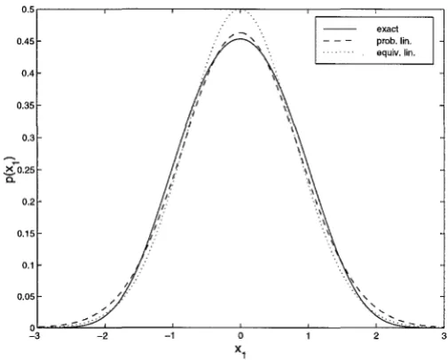
4.1 Approximate probability density functions for the response of the
linearly damped Duffing oscillator 45
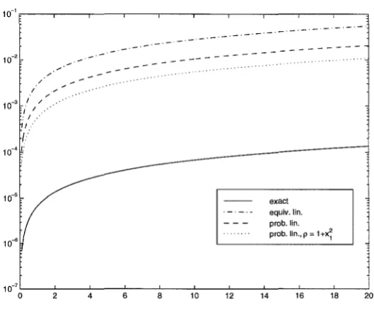
4.2 Fokker-Planck equation error for the linearly damped Duffing oscillator 46 4.3 Mean square estimation for the linearly damped Duffing oscillator for
small stiffness nonlinearities . . . 48 4.4 Mean square estimation for the linearly damped Duffing oscillator for
large stiffness nonlinearities . . . 49 4.5 Estimation of the higher moments of the response of the linearly
damped Duffing oscillator . . . 50 4.6 Stationary outcrossing rate estimation for the linearly damped
Duff-ing oscillator . . . 51 4.7 Estimation of the failure probability for the linearly damped Duffing
oscillator . . . 52 4.8 Weighting function used in the method of probabilistic linearization
to estimate the stationary outcrossing rate . . . 53 4.9 Stationary outcrossing rate estimation for the linearly damped
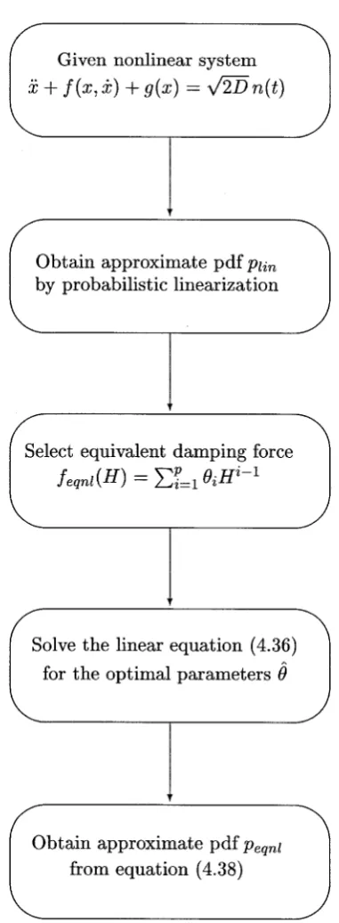
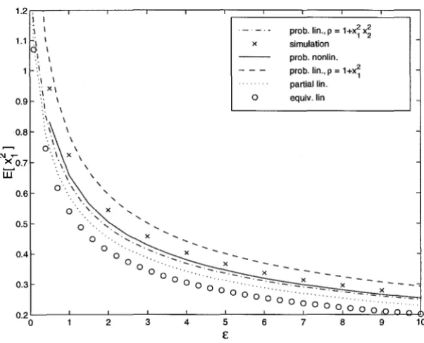
Duff-ing oscillator usDuff-ing weighted norm . . . 55 4.10 Flow chart illustrating steps in probabilistic nonlinearization method 64 4.11 Mean square values as a function of the stiffness nonlinearity for the
nonlinearly damped Duffing oscillator . . . 67 4.12 Mean square values as a function of the damping nonlinearity for the
4.13 Error in the Fokker-Planck equation as a function of stiffness nonlin-earity for the nonlinearly damped Duffing oscillator . . . 69
4.14 Error in the Fokker-Planck equation as a function of damping non-linearity for the nonlinearly damped Duffing oscillator . . . 69
4.15 Stationary probability density function approximation obtained by the method of equivalent linearization for the nonlinearly damped Duffing oscillator . . . . 0 • • • • • • • • • • • • • • • • 70
4.16 Stationary probability density function approximation obtained by the method of partial linearization for the nonlinearly damped Duff-ing oscillator . . . . 0 • • • • • • • • • • • • • • • • 71
4.17 Stationary probability density function approximation obtained by the method of probabilistic linearization for the nonlinearly damped Duffing oscillator . . . . 0 • • • • • • • • • • • • • • • • 72
4.18 Stationary probability density function approximation obtained by the method of probabilistic nonlinearization for the nonlinearly damped Duffing oscillator . . . . 0 • • • • • • • • • • • • • • • • 73
4.19 Probability density functionp(xl) for the nonlinearly damped Duffing oscillator for the various approximation methods. . . 7 4
4.20 Probability density functionp(x2) for the nonlinearly damped Duffing oscillator for the various approximation methods. . . 75 4.21 Fokker-Planck equation error for the quadratically damped oscillator 85 4.22 Mean square values for the quadratically damped oscillator . . . 86 4.23 Probability density function p(x1) for the quadratically damped
os-cillator . . . . 0 • • • • • • • • • • • • • • • • 87
4.24 Probability density function p(x2) for the quadratically damped os-cillator . . . . 0 • • • • • • • • • • • • • • • 88
4.25 Expected outcrossing rates for the quadratically damped oscillator 90
4.27 Error in the Fokker-Planck equation as a function of damping non-linearity for the nonlinearly damped Duffing oscillator . . . 93 4.28 Mean square values as a function of the stiffness nonlinearity for the
nonlinearly damped Duffing oscillator . . . 94 4.29 Mean square values as a function of the damping nonlinearity for the
nonlinearly damped Duffing oscillator . . . 95 4.30 Stationary probability density function PF obtained by the directly
approximating the Fokker-Planck equation for the nonlinearly damped Duffing oscillator . . . 96 4.31 Probability density functionp(x1) for the nonlinearly damped Duffing
oscillator. . . 97 4.32 Probability density function p( x2) for the nonlinearly damped Duffing
oscillator. . . 98 4.33 Outcrossing rate estimation for the nonlinearly damped Duffing
os-cillator . . . 99
5.1 Expected outcrossing rates for the linearly damped Duffing oscillator when all of the parameters are uncertain. . . 110 5.2 Expected outcrossing rates for the rolling ship when all of the
param-eters are uncertain. . . 114 5.3 FORM approximation to the failure surface 117 5.4 SORM approximation to the failure surface 118 5.5 Lognormal probability density functions for ( and Wn· 132 5.6 Safe and unsafe regions for
a;
<
0.15 133 5.7 Probability density function Pwn (wn) 135 5.8 Safe and unsafe regions in the transformed variables when Wn isdis-tributed as in Figure 5. 7 . . . 136 5.9 Probability density function for D. 137 5.10 Safe and unsafe regions for Vmax
=
10-5 . 138List of Tables
5.1 Mean square values for the linearly damped Duffing oscillator with one uncertain variable. . . 109 5.2 Mean square values for the linearly damped Duffing oscillator with
two uncertain variables. . . 109 5.3 Mean square values for the linearly damped Duffing oscillator when
all of the variables are uncertain. . . 109 5.4 Outcrossing rates for the linearly damped Duffing oscillator with one
uncertain variable. . . 111 5.5 Outcrossing rates for the linearly damped Duffing oscillator with two
uncertain variables. . . 111 5.6 Expected outcrossing rates for the rolling ship with one uncertain
variable having variance parameter, ()
=
0.1. . . 113 5.7 Expected outcrossing rates for the rolling ship with one uncertainvariable having variance parameter ()
=
0.2. . . 113 5.8 Comparison of SORM approximations for positive surface curvatures 126 5.9 Comparison of SORM approximations for negative surface curvatures 127 5.10 Comparison of SORM approximations with large negative curvature 128 5.11 Comparison of SORM approximations for large negative surfacecur-vature . . . . 129 5.12 Probability of mean square displacement exceeding ()~ax when Wn
and ( are lognormally distributed. . . 134 5.13 Probability of mean square displacement exceeding ()~ax when ( is
5.14 Probability of mean square displacement exceeding a~ax when D,
Wn, and ( are lognormally distributed. . . 137
5.15 Probability of outcrossing rate exceeding specified limit Vmax when (
and Wn are lognormally distributed. . . . 139
5.16 Probability of outcrossing rate exceeding specified limit Vmax when (
is lognormally distributed and Wn is distributed as in Figure 5.7. . . 140
5.17 Probability of outcrossing rate exceeding Vmax when D, Wn, and (are
Chapter 1
Introduction
Many structural and mechanical systems experience vibratory response as a result of environmental loads. Examples include the response of structures to earthquake and wind loadings, vibration of trains and automobiles traveling over rough surfaces, marine structures in waves and aircraft vibration due to turbulence. In all of these cases, there is a great deal of uncertainty in the loads that will be placed on the system over the course of its life.
While detailed knowledge of the forces the structure will be subjected to is not known, some information about the excitation is typically known. For example, measurements from previous earthquakes give engineers an estimate for the magni-tude, and sometimes the frequency content, of ground accelerations expected during an earthquake. Similar knowledge is often available for other environmental loads. Although this type of knowledge is useful, the actual excitations are often aperiodic and highly irregular and are not easily characterized. In addition to the complexity of the excitations, the loadings are not repeatable. Time histories recorded from different earthquakes and wind forces measured at different times often look very different.
aerospace systems.
For systems subjected to uncertain excitation, design and performance evalu-ation measures need to be formulated probabilistically. For example, due to the uncertainties in the excitation, no deterministic bounds can be placed on the mag-nitude of the response. The main objectives in analyzing systems subjected to un-certain excitations are to determine the probabilistic characteristics of the response and to calculate probabilities related to system performance, such as reliability. The probabilistic characteristics of the response can be determined analytically only for linear systems and a small class of nonlinear systems.
Over the last 40 years, a number of approximate methods have been developed for determining the probabilistic characteristics for the response of nonlinear sys-tems subjected to uncertain excitation. Several of these methods are discussed in chapter 3 and references containing more thorough reviews of the available methods are given. These methods generally provide good estimates to the mean square statistics for nonlinear systems, but often provide poor estimates for quantities re-lated to extreme values of the response, such as the reliability. New approximate methods are presented which are capable of providing good estimates to both the mean square statistics and the reliability for nonlinear systems.
In addition to the uncertainty in the excitation applied to structures, there is also uncertainty in the mathematical modeling of the system. Modeling uncertainty is inherent, as no mathematical model can completely describe the behavior of a physical system. The models developed are typically based on balance laws, experimental observations, or some combination of the two and often contain a number of parameters, such as elastic moduli, damping ratios, natural frequencies, modeshapes, etc. The values of these parameters which will give the best agreement between the response of the model and that of the physical system are not known precisely, and the resulting uncertainty is referred to as parametric uncertainty.
and this worst-case performance value is used for design and analysis purposes. One problem with this approach is that it can be highly conservative. This is especially true as the number of uncertain parameters becomes large, since the likelihood of the parameters achieving the worst-case performance may be extremely low. Another difficulty with this approach is finding the bounded domain in which the parameters are assumed to lie. In many cases, it is difficult to put hard bounds on parameter values.
Another approach for dealing with modeling uncertainty is to use probabilistic methods. In order to use probabilistic methods for parametric uncertainty, proba-bility must be interpreted in a Bayesian sense, as a multi-valued logic for plausible reasoning subject to certain axioms (Jeffreys 1961; Box and Tiao 1973; Beck 1989; Beck 1996), since the relative frequency interpretation of probability does not make sense for parametric uncertainty. The probability density function for the param-eters represents the relative plausibility of the paramparam-eters based on the engineer's knowledge, experience and judgment. One of the problems with using probabilistic methods is the computational difficulties that often arise. Typical problems that arise require computing integrals over the parameter space, which may be high dimensional. Straightforward numerical integration becomes computationally pro-hibitive when there are more than a few uncertain parameters, and approximate methods are required.
1.1
Organization of Thesis
An overview of the mathematics of stochastic processes and stochastic differen-tial equations is presented in chapter 2, providing the background for the material covered in chapters 3 and 4. The Fokker-Planck equation is introduced and there-lationship between stochastic differential equations and the Fokker-Planck equation is illustrated. The concept of reliability and the classical first passage problem are covered, and some issues related to numerical solutions to the Fokker-Planck and backward Kolmogorov equation are discussed.
Chapter 3 contains a review of a number of analytical methods available for in-vestigating the response of structural systems under random excitation. After some background and historical notes on random vibration theory, the chapter begins with a discussion of systems for which analytical solutions can be obtained for the probability distribution of the response. The number of systems for which analyti-cal solutions are available is rather limited and in the remaining sections, a number of approximate techniques based on approximating the stochastic differential equa-tions are reviewed. The review is not intended to be exhaustive, but rather to review some of the well-known methods, with more emphasis being given to those methods which will be used for illustration purposes in chapter 4.
Chapter 2
Stochastic Processes, Stochastic Differential
Equations, Fokker-Planck Equation, and
Reliability of Stochastic Dynamical Systems
This chapter contains a brief overview of some of the theory of stochastic processes, with particular emphasis on Markov processes. The Fokker-Planck equation as-sociated with a Markov process is introduced in section 2.3. Some background on stochastic differential equations and stochastic integrals is presented in sections 2.4-2.6. In section 2.7, the relationship between stochastic differential equations and the Fokker-Planck equation is illustrated. section 2.8 presents an introduction to relia-bility for stochastic dynamical systems as well as the classical first passage problem. A review of numerical solutions to the Fokker-Planck equation is given in section 2.9 and some concluding comments are made in section 2.10.
2.1
Stochastic Processes
variables Xi
=
x(ti)(2.1)
exists for all n E
z+.
Knowledge of the probability density functions (2.1) would provide a complete description of the stochastic process.Note that the probability density functions defined by (2.1) will depend on the mathematical model for the stochastic process. Therefore, the probability density functions should technically be written as
where
M
denotes the model for the stochastic process. For brevity, this dependence will be dropped in the notation.Conditional probability density functions can be deduced from (2.1) and Bayes's rule (Feller 1968) by
While this definition is valid regardless of the ordering of the times, the times will be considered to be increasing as the index increases, i.e.,
2.2
Markov Processes
Equation (2.2) is known as the Markov condition and it implies that all prob-ability density functions can be written in terms of simple conditional probprob-ability density functions of the form p(x,
t
I
y, s) with s<
t,
since given any probability density function p(xn, tn; ... ; x1, t1), repeated application of the Markov condition and Bayes' rule givesn-1
p(xn,tn; ... ;x1,t1) =p(x1,t1) ITp(xk+l,tk+llxk,tk)
k=l
2.2.1 The Lindeberg Condition and Continuity of Stochastic
Pro-cesses
While stochastic processes can only be described probabilistically, a question of interest is whether or not samples of the process are continuous. The stochastic processes studied in this work are the response of oscillatory systems to stochastic excitation, for which the sample paths are expected to be continuous.
A conditional probability density function is said to satisfy the Lindeberg
condi-tion on a domain 1) C IRn+l if for any E
>
0(2.3) lim
!
f
p(x, t+
~t
1 y, t) dx=
o
Llt--+0 ut }llx-yll><for all (y, t) E V. It can be shown that if the conditional probability density function for a Markov process satisfies the Lindeberg condition on IRn+l, then the sample paths are continuous with probability one (Gihman and Skorohod 1975).
2.3 The Fokker-Planck Equation
process. If, in addition to the Lindeberg condition (2.3), the conditional probability density functions of a Markov process satisfy the following for all E
>
0(2.4a) lim :
r
(x- y)p(x, t+
~t
I
y, t) dx = a(y, t)+
O(E)Llt-+O ut J11x-yll<<
(2.4b) lim :
r
(x- y)(x- y f p(x, t+
~t
I
y, t) dx=
D(y, t)+
O(E)Llt-+0 ut }llx-yll<<
uniformly in y, t and E, then the probability density functions will also satisfy the
Fokker-Planck equation
(2.5) ap(x,tiy,s) =L( at x, p x, t) ( tl y,s )
where L(x, t) is the forward Kolmogorov operator defined by
(2.6) L(x, t) '1/J(x)
= _
t
a (ai(x, t)'lj;(x))+
~
t t
a
2(Dij(x, t)'lj;(x))
i=l axi 2 i=l j=l axi ax j
for all 'ljJ E C2(1Rn). The vector a(y, t) is called the drift vector of the process and
the matrix D(y, t) is called the diffusion matrix.
The Fokker-Planck equation is named after the work ofFokker (1915) and Planck
(1917) and is often called the Fokker-Planck-Kolmogorov equation due to the con-tributions of Kolmogorov (1931). For a derivation of the Fokker-Planck equation, consult Gardiner (1994) or Lin and Cai (1995). Further information regarding the Fokker-Planck equation and applications can be found in the books by Risken (1989)
and Soize (1994).
2.4
Stochastic Differential Equations
Stochastic differential equations are differential equations containing terms which are modeled as stochastic processes. They were first investigated by Langevin (1908)
Stochastic differential equations are often written in the form
(2.7)
d l
dx(t) = x(t) = f(x, t)+
B(x, t)n(t)where x(t), f(x, t) E IRn, B(x, t) E IRnxm and n(t) E IRm is the stochastic term, which is often assumed to be rapidly fluctuating. The mathematical idealization of such a term is that for r
-I
0, n(t) and n(t+
r) are statistically independent. The mean n(t) is usually taken to be zero, since any nonzero mean can be absorbed intof(x, t). The requirements of zero mean and statistical independence can be written
as
E[n(t)] 0
(2.8)
where E denotes mathematical expectation and I is the m x m identity matrix. Choosing the identity matrix is merely for convenience since any other amplitude can be accounted for in B(x, t). Excitation satisfying the conditions (2.8) is known as white noise.
While excitation having the properties (2.8) satisfies the requirement of sta-tistical independence, it gives n(t) an infinite variance. A more realistic model is that
where Tc is the correlation time of the excitation. This gives statistical independence
for r
»
Tc· Then, white noise could be taken as the limit as Tc -+ 0. In practice, itis not easy to evaluate these limits (Gardiner 1994) and an alternative approach is to rewrite (2.7) as an integral equation
(2.9) x(t)
=
x(t0 )+
{t
f(x(s), s) ds+
{t
B(x(s), s) n(s) ds.It can be shown (Gardiner 1994) that if n(s) satisfies the properties (2.8), then
(2.10)
lot
n(s) ds=
w(t)where w(t) is the multivariate Wiener process having properties
(2.11a)
(2.1lb)
E[w(t)-w(s)] = 0
E [(w(t)- w(s)) (w(t)- w(s))TJ = Ilt-
sl
for all t, s E IR. Equation (2.10) shows that n(t) as defined by (2.8) is like the derivative of the Wiener process, but the latter is not differentiable with probability one (Wiener 1923). Therefore, the proper interpretation of (2.7) is as the integral equation (2.9). Introducing
(2.12) dw(t)
=
w(t+
dt) - w(t)=
n(t)dtthe integral equation (2.9) can be rewritten as
(2.13) x(t)
=
x(to)+
{t
f(x(s), s) ds+
{t
B(x(s), s) dw(s).ito
ito
The second integral in (2.13) is a stochastic integral and is defined in the section 2.5.
2.4.1 Some Comments About White Noise
spectra for ocean waves (Hu and Zhao 1993) and Davenport's spectrum for wind excitation (Davenport and Novak 1976).
2.5
Stochastic Integrals of
Ito
and Stratonovich
In section 2.4, it was shown that the proper interpretation of a stochastic differential equation is as an integral equation, involving a term of the form
(2.14)
1
t B(x(s),s)dw(s). toIntegrals of the form (2.14) are called stochastic integrals and are defined as a kind of Riemann-Stieltjes integral. The time interval [to, t] is partitioned into n subintervals
[ti,tj] with
to
<
t1< · · · <
tn-1<
tand the integral is defined as a limit of partial sums. However, due to the rapid fluctuations of the Wiener process, the value of the integral depends on where the integrand is evaluated in each subinterval. Two choices have shown to be useful in practice, and the resulting integrals are known as Ito and Stratonovich integrals, based on the work of Ito (1951) and Stratonovich (1963).
2.5.1 The
Ito
IntegralThe Ito stochastic integral is defined by
(2.15)
1
t B(x(s), s) dw(s)=
ms-limt
B(x(ti_l), ti-l) (w(ti)- w(ti-1))to n---+oo i=l
where ms-lim is the mean-square limit (Gardiner 1994). Notice that in each subin-terval, b(x(t), t) is evaluated at the previous time ti-l, and, by the properties of
the Wiener process, b(x(ti-1), ti-l) is statistically independent of the increment
of applications, and it will be seen that the Fokker-Planck equation corresponding to a stochastic differential equation is easily obtained if the integral in (2.13) is an Ito integral. A drawback to the Ito integral is that some of the resulting properties, such as the change of variables formula, are different from ordinary calculus (Soong and Grigoriou 1993).
2.5.2 The Stratonovich Integral
The Stratonovich integral, denoted here by S
J,
is defined by(2.16)
l.
t ( ) .Ln
(x(ti)+
x(ti-1) )S b(x(s), s) dw s
=
ms-hm B , ti-l (w(ti)- w(ti-1)).to n-+oo i=l 2
Notice that the difference between the Ito integral and the Stratonovich integral is where the integrand is evaluated in each interval. Also notice that if b(x(s),s) is independent of x, the two integrals will be equivalent. The Stratonovich integral has the advantage that many of its properties, including the change of variables formula, are the same as those of ordinary calculus.
2.6
Ito and Stratonovich Stochastic Differential
Equa-tions
It was shown in section 2.4 that the proper interpretation of the stochastic differen-tial equation (2. 7) is as the integral equation (2.13). The integral equation is often written in differential form as
(2.17) dx(t)
=
f(x(t), t) dt+
B(x(t), t) dw(t).If the integral in (2.13) is interpreted as an Ito [Stratonovich] integral, the differential equation (2.17) is called an Ito [Stratonovich] stochastic differential equation.
appli-cation.
2.6.1 Relation Between
Ito
and Stratonovich SDE's
In section 2.7, it is shown that the Fokker-Planck equation corresponding to a stochastic differential equation can be obtained easily if the differential equation is thought of as an Ito equation. However, Stratonovich equations are a more nat-ural choice for an interpretation which assumes the excitation is a physical noise with a finite correlation time, which is allowed to become arbitrarily small after calculating desired quantities (Gardiner 1994). Stratonovich equations are also pre-ferred in some applications, since the rules of ordinary calculus can be applied to Stratonovich equations, while the rules of the Ito calculus are different. For these reasons, it is useful to be able to convert an equation of one type into the other type.
It can be shown (Gardiner 1994) that the Ito SDE
dx(t) =
f
1 (x(t), t) dt+
B(x(t), t) dw(t)is equivalent to the Stratonovich SDE
dx(t)
=
f
8(x(t), t) dt
+
B(x(t), t) dw(t)where
(2.18)
f
~s
=
J!
~_!
2~~
L.,; L.,; Bk·f)Bij Jax .
j=lk=l k
2. 7
Connection between Stochastic Differential
Equa-tions and the Fokker-Planck Equation
An ordinary differential equation is said to be memoryless if the solution for fu-ture times can be obtained from the present state independently of the manner in which the present state was reached. The solution, x(t), to a memoryless stochas-tic differential equation of the form (2.17) is a Markov process. Intuitively this is clear since the future response depends only on the present state and not on past values, therefore the state-transition probability density functions should also be independent of the previous state values. A rigorous proof of this result can be found in Arnold (1974). Since the solution to the differential equation is a Markov process, the state-transition probability density functions for x(t) are governed by a Fokker-Planck equation. It is easiest to determine the corresponding Fokker-Planck equation if the differential equation is interpreted as an Ito equation. Stratonovich equations can be handled by converting to the equivalent
Ito
equation using the Wong-Zakai correction terms (2.18).It can be shown (Gardiner 1994; Lin and Cai 1995; Caughey 1971) that the response x(t) to an
Ito
equationdx(t) = f(x(t), t) dt
+
B(x(t), t) dw(t),is a Markov process with drift vector a(x, t)
=
f(x(t), t) and diffusion matrixD(x, t)
=
B(x(t), t)BT(x(t), t). Therefore, from (2.5) and (2.6), the state-transitionprobability density function p(x,
t
I
y, s) satisfies the following Fokker-Planck equa-tion(2.19)
ap(x, t 1 y, s)
= _
t
a (fi(x, t)p(x, t 1 y, s))at i=l axi
+
~ ~ ~ ~ 82 (Bik(x, t)Bkj(x, t)p(x, tI
y, s)).2 L.._.. L.._.. L.._.. ax . ax .
i=l j=l k=l 2 J
difficult to solve, and often the long-term, or steady-state response of the system is of interest. If f(x,
t)
and B(x,t)
do not depend explicitly ont,
the steady-state probability density function p(x) satisfies the stationary, or reduced, Fokker-Planck equation(2.20) _
~
& (fi(x)p(x))+!
~
~
~
&2
(Bik(x)Bkj(x)p(x))
=
O.L...J ax· 2 L...J L...J L...J &x·&x.
i=l z i=l j=l k=l z J
In terms of the forward Kolmogorov operator defined by (2.6) with a(x) = f(x) and
D(x)
=
B(x)BT(x), the stationary Fokker-Planck equation can be written in the simple form(2.21) L(x)p(x)
=
0.Even for the stationary Fokker-Planck equation (2.21), there are very few known solutions for nonlinear systems, as discussed in section 3.1. Some comments on numerical solutions to the Fokker-Planck equation are given in section 2.9 and a number of new methods for approximating solutions to the stationary Fokker-Planck equation are given in chapter 4.
2.7.1
Differential Equations with Memory
2.8 Reliability and the First Passage Time
One of the most important properties of a dynamical system subjected to stochastic excitation is its reliability. Due to the uncertainty in the excitation, no deterministic bounds can be set on the response amplitude, but the probability that the states remain in a "safe" or "acceptable" domain is often of interest. Typically, a safe set, S, and a failure set, F, are defined such that the system performance is acceptable
if x E S and unacceptable if x E F. The reliability is then defined by
R(xo, T) = P( x(t) E S lx(O) = xo) for all t E
[0,
T]where R is the reliability, P( ·) denotes probability and
[0, T]
is the time interval of interest. Associated with the reliability is the failure probability, Pf, which is given byPt(xo, T)
=
P( x(t) E F lx(O)=
xo) for some t E [0, T].Clearly, Pt(xo, T)
=
1-R(xo, T), provided that the sets Sand Fare complements, as usually defined.A classical problem associated with reliability theory is the first passage problem.
Letting T be the time at which x(t) first leaves S, the first passage problem is to
determine the probability distribution forT, i.e., to determine P(T ~ t) for all times
t
>
0. From the above definitions, it can easily be seen that P(T ~ t) given thatx(O) = xo is equal to R(xo, t).
It can be shown (Gardiner 1994) that R(xo, t) satisfies the backward Kolmogorov equation
(2.22)
BR~t
t) = L*(xo, t)R(xo, t)where L*(x0 , t), the adjoint of the forward Kolmogorov operator, is the backward
Kolmogorov operator. If a(x, t) is the drift vector and D(x, t) is the diffusion matrix
(2.23)
Assuming that S is a simply connected region with boundary aS, the initial condi-tion for the backward Kolmogorov equacondi-tion (2.22) is
(2.24) R(xo,O)
=
1 for X0 E Sand the boundary condition is
R(xo, t)
=
0 for Xo E aS for all t> .
The first passage problem for second-order systems subjected to white noise exci-tation was first posed by Yang and Shinozuka (1970) as an initial-boundary value problem for the backward Kolmogorov equation and by Crandall (1970) for the Fokker-Planck equation. Fischera (1960) proved the well-posedness of these prob-lems.
Unfortunately, analytical solutions of the backward Kolmogorov equation exist only for the simplest scalar systems as illustrated by Darling and Siegert (1953). Therefore, even for linear systems, approximate methods are required for estimating the reliability. Approximate methods based on outcrossing rates are discussed in section 3.2.2.
2.9 Numerical Solution of the Fokker-Planck and
Back-ward Kolmogorov Equations
Due to the limited number of analytical solutions available for the Fokker-Planck and backward Kolmogorov equations, a number of approaches have been made to obtain numerical solutions to these equations.
a second-order linear oscillator (Chandiramani 1964; Crandall et al. 1966). In their method, the safe region in the state space was divided into cells, and the probability was diffused from cell to cell in each time based on the analytical solution for the state-transition probability density function for the linear oscillator. Later, Sun and Hsu (1988, 1990) developed a generalized cell mapping method to obtain solutions to the first passage problem for nonlinear second-order oscillators. Here, short-time simulations were used to map the probability from cell to cell in each time step.
Another approach to obtaining approximate solutions is based on Galerkin's method. Atkinson (1973) used this method to investigate stationary solutions of the Fokker-Planck for second-order nonlinear systems. The trial functions were based on the eigenfunctions of the forward Kolmogorov operator for the linear systems. The method was extended to investigate nonstationary response (Wen 1975) and Bouc-Wen type hysteretic systems (Wen 1976). A Galerkin approach using locally defined Gaussian probability density functions was developed by Kunert (1991). One of the difficulties in applying this approach is obtaining good trial functions, as discussed in Wen (1975).
Finite element solutions to the stationary Fokker-Planck equation for second-order nonlinear systems have been obtained by Langley (1985) and Langatangen (1991). One of the main difficulties associated with numerically solving the sta-tionary Fokker-Planck equation is satisfying the global normalization condition for the probability density function. An alternative approach based on solution of the Chapman-Kolmogorov equation has been developed by Naess and Johnsen (1991).
All of the numerical methods so far proposed require a significant amount of computational time. In addition, the solutions obtained for the probability density function are not typically in a convenient form for calculating statistical quantities of interest, such as moments and stationary outcrossing rates. In chapter 4, efficient methods for approximating the solutions to the stationary Fokker-Planck equation are developed.
2.10 Final Remarks
It has been shown that given any stochastic ordinary differential equation, the Fokker-Planck equation is a (deterministic) partial differential equation governing the evolution of the state transition probability density function. Both stochastic differential equations and the Fokker-Planck equation have been shown to be useful in practice; the following quotation is from Gardiner (1994)
There are many techniques associated with the use of Fokker-Planck equations which lead to results more directly than by direct use of the corresponding stochastic differential equation; the reverse is also true. To obtain a full picture of the nature of diffusion processes, one must study both points of view.
Chapter 3
Random Vibration Theory
Random vibration theory is the study of the vibrational response of mechanical and structural oscillatory systems under uncertain dynamic excitation. The uncer-tain excitations, for example wind or earthquake loads, are typically modeled as stochastic processes, leading to stochastic differential equations for the response.
Vibration response due to stochastic excitation was first studied in the mid 1950's in the aerospace industry. Fuselage panels near jet engines were experiencing fatigue cracks due to the acoustic excitation from the jet exhausts. When the excitation from the engines was studied, it was found to be rapidly fluctuating, aperiodic, and lacked repeatability from one experiment to the next (Clarkson and Mead 1972). Some other early problems studied were the effects of atmospheric turbulence on aircraft (Press and Houboult 1955) and the reliability of payloads in rocket-propelled vehicles (Bendat et al. 1962). In all of these cases, the response was sufficiently complex and irregular that a probabilistic or statistical approach was found to be much more useful than traditional deterministic approaches.
Vanmarcke 1976; Park 1992; Papadimitriou and Beck 1994; Schueller et al. 1994) and vibration of vehicles traveling over bumpy surfaces (Newland 1986; Schiehlen 1986; Ushkalov 1986; Hunt 1996). Several textbooks giving a good overview of the subject have been written, e.g., (Crandall and Mark 1963; Lin 1967; Nigam 1983; Roberts and Spanos 1990; Newland 1993; Soong and Grigoriou 1993; Lin and Cai 1995; Lutes and Sarkani 1997).
In random vibration studies, the system response is a stochastic process, and the goal of the engineer is to determine as much probabilistic and/or statistical infor-mation about the process as is possible. If the state-transition probability density functions p(x, tixo, to) could be obtained for all times t
>
to, all probabilistic and statistical information about the system could be determined from the probability density functions and the system's initial conditions. Unfortunately, for most non-linear systems of interest, there is no known way to determine the state-transition probability density function, or even the stationary probability density functionp(x). A summary of systems for which analytical solutions to the Fokker-Planck
equation are known is given in section 3.1. Often, statistical parameters for the response, such as moments and expected outcrossing rates, are of interest, as dis-cussed in section 3.2. section 3.3 presents some approximate methods which have been developed based on approximating the stochastic differential equations.
3.1
Exact Solutions in Random Vibration Theory
relationships between the system and excitation parameters which are unlikely to be met in practice. A more complete review of the known solutions can be found in Lin and Cai (1995).
3.1.1 Linear Systems with Gaussian White Noise Excitation
The state-transition probability density function can be obtained for time-invariant linear systems of any dimension subjected to additive Gaussian white noise (or lin-early filtered Gaussian white noise). Such linear dynamical systems under additive stochastic excitation can be written in the form
dx(t)
=
Ax(t) dt+
B dw(t)where A E IRnxn, BE IRnxm and w(t) E IRm is the standard Wiener process having the properties in (2.11a) and (2.11b). In this case, the state-transition probability density function p( x, tixo, to) can be obtained by solving a (deterministic) Lyapunov matrix differential equation (Lin 1967).
Without loss of generality, to can be taken to be zero and the transition proba-bility density function is given by
p(x, tixo)
=
12 1 exp(-!(x-
xo)T p-1(t)(x- xo))(21rt y'detP(t) 2
where P(t) is the solution to the differential Lyapunov equation
P(O) Po.
Here, Po = E[xox~] is the covariance matrix for the initial state x0 . If the linear
covariance matrix
P
can be obtained by solving the algebraic Lyapunov equationand the stationary probability density function is given by
3.1.2 Stationary Solutions for Nonlinear
Systems
Exact solutions to the stationary Fokker-Planck equation have been obtained for a number of single degree-of-freedom nonlinear oscillators. The first solutions ob-tained (Andronov et al. 1933) were for single degree-of-freedom oscillators with linear damping and nonlinear stiffness. Solutions for more general nonlinear sin-gle degree-of-freedom oscillators, including systems with energy-dependent damp-ing were obtained by Caughey and Ma (1982). The class of systems with known solutions was extended through the concept of detailed balance by Yong and Lin (1987) and further generalized by Lin and Cai (1988) through a generalization of Stratonovich's method of stationary potential.
The single degree-of-freedom systems with energy-dependent damping that will be of interest in later sections can be written in the form
(3.1)
x
+
f(H)x+
g(x)=
JWn(t)where
(3.2) H(x, x)
=
~
·2+
Jor
g(~) d~
is the Hamiltonian and n(t) is Gaussian white noise. If the following techni-cal conditions are met: H(x,x), j(H) E C2, H(x,x)
>
0, 3H0 such thatH
2::
H0 =? f(H)>
0, and f'(H)/ f2
the stationary Fokker-Planck equation associated with (3.1) is
(3.3)
(
1 {H(x,x) )
p(x,x)
=
aexp - D lo f('T!)d'T!where a is a normalization constant (Caughey and Ma 1982).
There are very few solutions to the stationary Fokker-Planck equation for multi-of-freedom systems. Even for multi-multi-of-freedom analogs of single degree-of-freedom systems with known solutions, solutions cannot typically be found, and in the few cases where analytical solutions are known, these solutions typically require restrictive relationships between the system and excitation parameters unlikely to be met in practice. Further information on known solutions for multi-degree-of-freedom systems can be found in the books by Soize (1994) and Lin and Cai (1995).
Unfortunately, even for single degree-of-freedom nonlinear oscillators, many of the systems of interest are not of the solvable form. Although the known solutions are not directly applicable to these systems, they have been very helpful in testing the accuracy of proposed approximation methods. Additionally, these solutions can be used to approximate the solution of other nonlinear systems, as in sections 3.3.2, 4.3 and 4.4.
3.2
Statistical Parameters of Interest
3.2.1 Moments
Some of the most important properties of a stochastic process are characterized by its moments, particularly the first and second moments. If x(t) is a scalar stochastic process with probability density function p(x, t), the nth_order moment
Similarly, for vector processes, joint moments can defined by
. . k
mijk ... = E[xix~x3 .. . ].
Much of the information about a stochastic process is contained in the first and second order moments. For example, for Gaussian distributed processes, all probabilistic and statistical information can be determined from knowledge of the first and second-order moments. The first moments give the mean values of the response and the second moments give the mean square values, which typically provide a measure of the average energy in the system. Additionally, knowledge of the first two moments of a stochastic process enable upper bounds to be placed on the reliability of the response through the generalized Tchebycheff's inequality. If
the random process x(t) has mean ftx(t) and variance O";(t) and the derivative of
x(t) has variance O"~(t), the generalized Tchebycheff's inequality (Lin 1967) gives
(3.4)
1
11T
P( lx(t)- J.tx(t)l
2::
E for some t E [0, T]):S: -
2(O";(o)
+
O";(r))
+
2 O"x(t)O"x(t)dt2€ E 0
for all E
>
0. The left-hand side in (3.4) is the probability offailure associated withthe safe set S(t)
=
{x E IR : lx- J.tx(t)i<
E}. While (3.4) is useful as an upper bound, it is often highly conservative in practice.3.2.2 Expected Outcrossing Rates and Reliability Estimation
While mean square values provide a lot of information about the response, often the primary goal is to determine the reliability of the system. As discussed in section 2.8, reliability is the probability that the response variables remain in a safe or acceptable domain during a time interval of interest. In vibration applications, the safe domain is often chosen to be a region where displacements stay within some prescribed limits.
os-cillatory systems subjected to stationary random excitation, there are well-known methods for estimating the reliability based on expected outcrossing rates. The original work in this area was done by Rice (1944) and a number of extensions have been developed since then.
Consider a single degree-of-freedom oscillator subjected to stationary white noise excitation
x
+
f(x,x)+
g(x)=
v2Dn(t).In one of the simplest cases, the safe domain is the regionS= {(x,x) E IR2 : x
<
b}for a given b
>
0. Letting p(x,x) be the stationary probability density function for the Markov process x(t), the expected crossing rate of the threshold b is given by Rice's formula {Rice 1944){3.5) v
=
fooo
xp(b, x)dx.Typically, b
»
JE1X2T
so that threshold crossings are rare and the resulting failure probability is low. If the threshold crossings are assumed to arrive independently, it follows that the threshold crossings are Poisson distributed in time and the prob-ability of failure is given by{3.6) Pj(t) = 1- exp(-vt)
from which the reliability is given by R = exp( -vt). Equation {3.6) was first suggested by Coleman (1959) for the reliability of structures against first-excursion failures.
Wright 1985; Roberts 1978a; Roberts 1978b). However, for finite values of b, it is well-known that the threshold crossings do not arrive independently, and that they tend to occur in "clusters" (Lin 1967). Despite this shortcoming, equation (3.6) is still useful as efficient way to get an order-of-magnitude estimate of the failure probability.
3.3 Approximate Methods Based on Stochastic
Differ-ential Equations
Due to the limited number of analytical solutions available for nonlinear systems under stochastic excitation, a number of approximate methods have been devel-oped. In this section, some of the well-known methods based on approximation of the stochastic differential equations are presented, with more attention given to those methods which are used later for illustrating the new approximate methods developed in chapter 4.
3.3.1 The Method of Equivalent Linearization
The most popular method used in the analysis of nonlinear systems is the method of equivalent linearization. It was originally developed by Booton (1954) and Caughey (1959a, 1959b) for single degree-of-freedom systems and was later generalized for multi degree-of-freedom systems (Foster 1968; Iwan and Yang 1972; Iwan 1973; Atalik and Utku 1976).
Single Degree-of-Freedom Systems
In the method of equivalent linearization, the response of the nonlinear stochastic differential equation of interest
is approximated by that of a linear system
(3.8)
The parameters of the linear system (3.8) are selected to provide the best approx-imation to the nonlinear system (3. 7). To do this, the mean square equation error is minimized, i.e. /3eq and w;q solve
(3.9)
Performing the minimization, the optimal parameters are found to be
(3.10a)
(3.10b)
If n(t) is modeled as Gaussian white noise with properties given by (2.8), the sta-tionary probability density function for the linear system can easily be obtained as
( . ) /3eq Weq ( /3eq
W~q
2 /3eq . 2 )p X lin, X[in = 27r D exp - 2D X tin - 2D X tin .
The probability density function for the nonlinear system is then approximated by that of the linear system.
Multi Degree-of-Freedom Systems
The multi degree-of-freedom analog of (3.7) is
(3.11)
where x(t) E IRn, n(t) E IRm, BE IRnxm, M is a symmetric, positive-definite n x n
equation is replaced by a linear system
(3.12)
so that the mean square equation error is minimized. To minimize the error, the
n x n matrices Ceq and Keq are chosen to solve
(3.13)
where
II · II
is the Euclidean norm on IRn. Using the identity that for x, y E IRn andA E IRnxn,
a
r aA (Ax,y)=
xyand differentiating (3.13) with respect to Ceq and Keq gives
(3.14)
where
Since Pis a function of Keq and Ceq, equation (3.14) contains 2n2 coupled, nonlinear equations for the unknown elements of Keq and Ceq· A simple iterative procedure is available in the case of Gaussian white noise excitation.
Iterative Procedure for Multi Degree-of-Freedom Systems
When n(t) is modeled as Gaussian white noise, P can be obtained as the solution of the algebraic Lyapunov equation
where
)
The iterative procedure is as follows
1. Start with an initial estimate of P
2. Use this Pin (3.14) to obtain Keq and Ceq (and hence Aeq)
3. Use Aeq from step 2 and solve (3.15) for P
4. Repeat steps 2 and 3 until convergence
The probability density function for the nonlinear system is again approximated
by that of the linear system. Letting Ynl = (x;:1,
x;:
1)T, the stationary probabil-ity densprobabil-ity function is given by the multidimensional Gaussian probabilprobabil-ity densprobabil-ityfunction with covariance matrix P
~ 1 ex ( - -1 T p-1 )
P(Ynl) (21r)n vdet p P 2 Ynl Ynl ·
Note that in the iteration procedure, step 2 involves evaluating expectations
and matrix multiplication and step 3 requires solution of a linear equation. Both of
these steps can be done efficiently, and, except for simulation methods (discussed
in section 3.3.4), this is basically the only method that has been able to obtain
approximations for nonlinear systems in many dimensions.
3.3.2 Approximation by Nonlinear Systems
The equivalent linearization method can be easily and efficiently applied to many
nonlinear systems of interest. The method generally gives reasonably good
approx-imations to mean square values, even for systems with large nonlinearities.
How-ever, the approximate probability density function obtained is Gaussian, while the
errors when approximating quantities related to extreme values of the process, such as reliability or stationary outcrossing rates.
In an effort to obtain better accuracy than that obtained by the method of equiv-alent linearization, some equivequiv-alent nonlinearization methods have been developed. The basic idea for equivalent nonlinearization was originally suggested by Caughey and particular problems have been investigated by Lutes (1970), Kirk (1974), and Caughey (1986). A special case of equivalent nonlinearization in which computa-tions can be done rather efficiently, termed partial linearization (Elishakoff and Cai 1993), has since been developed. In these methods, the nonlinear differential equa-tion is approximated by a different nonlinear system which has a known staequa-tionary probability density function. Since the approximate system is nonlinear, the approx-imate probability density function obtained will be non-Gaussian, and the hope is that this will lead to better approximations, particularly for reliability. The appli-cability of these methods is primarily limited to single degree-of-freedom systems, since the approximate system must be one for which the stationary Fokker-Planck equation can be solved.
Partial Linearization
In the method of partial linearization (Elishakoff and Cai 1993), the response of the nonlinear single degree-of-freedom system
(3.16)
is approximated by the response of the nonlinear system with linear damping
If the excitation, n(t), is modeled as Gaussian white noise, the stationary probability density function for the response of (3.17) is
(3.18) ( · ) _ ( f3eq G( ) f3eq . 2 )
P Xplin, Xplin - a exp -
D
Xplin-2D Xplin
where a is a normalization constant and
(3.19)
As in the case of equivalent linearization, the equivalent damping parameter, f3eq is given by minimizing the mean square equation error
Performing the minimization gives
(3.20) (3 eq-_ E[xplin f(xplin, Xplin)]
E[
·2 ]xplin
and the probability density function for the nonlinear system is approximated by (3.18) with f3eq as given by (3.20).
For single degree-of-freedom systems, this method can be applied efficiently, since obtaining the optimal parameter only requires computing expectations. Also notice that the formula (3.20) for the optimal damping parameter is the same as the formula obtained by the method of equivalent linearization (3.10a).
Equivalent Nonlinearization
In the method of equivalent nonlinearization, the nonlinear system chosen to ap-proximate (3.16) is of the form
where His the Hamiltonian as given in (3.2) and feqnt(H) is a specified function of the Hamiltonian. Note that the partial linearization method is a special case of this method, obtained by choosing feqnt(H)
=
/3eq· The stationary probability densityfunction for the equivalent nonlinear system (3.21) is
Typically, feqnl(H) is taken to be a polynomial in H and the coefficients of the polynomial are chosen to minimize the mean square equation error. For example, if
feqnl(H)
=
L::f=l
(}iHi-l, then the minimization condition is(3.22)
This results in a set of nonlinear algebraic equations for the parameters which usu-ally need to be evaluated numericusu-ally. Note that the expectations which need to be evaluated are with respect to the probability density function for the equiva-lent nonlinear system, and numerical integration is often required to evaluate the expectations. Thus, at each iteration in the minimization procedure, numerical integration is required to evaluate the expectations, making this method more com-putationally expensive than either the method of equivalent linearization or the method of partial linearization.
3.3.3 Closure Techniques
are referred to as closure methods.
In one of these methods, Gaussian closure, only second-order moments are de-termined, and the relationship between higher-order and lower-order moments is assumed to be the same as for Gaussian probability density functions. It can be shown that this method gives the same results as equivalent linearization. Non-Gaussian closure techniques were first introduced by Crandall (1980). One of the most frequently used non-Gaussian closure techniques is the cumulant-neglect clo-sure method. Here, the equations for the cumulants are obtained, and all cumulants above a certain order are assumed to be zero. This yields a system of nonlinear, algebraic equations for the unknown moments, which can be solved numerically. The number of equations to solve grows very rapidly as the dimension of the state is increased as well as when the order of the approximation is increased, making this method computationally expensive for multi-degree-of-freedom systems.
While these methods are often able to provide better estimates to the moments than the method of equivalent linearization, the methods do not provide any esti-mate of the probability density function for the system, and hence provide no way to approximate outcrossing rates or reliability. Some methods have been proposed to determine an approximate probability density function based on the moments, including Edgeworth series (see, e.g., Roberts and Spanos (1990)) and the principle of maximum entropy (Trebicki and Sobczyk 1996), but little work has been done to determine the accuracy of such methods for determining reliability.
3.3.4 Other Methods
A number of other approximate methods based on approximating the stochastic dif-ferential equations have been developed, including perturbation methods, stochastic averaging, and dissipation energy balancing. More details on these methods can be found in the books by Lin and Cai (1995), Soong and Grigoriou (1993), and Roberts and Spanos (1990).
Chapter 4
Approximate Methods for Random Vibrations
Based on the Fokker-Planck Equation
All of the methods presented in chapter 3 were based on writing stochastic dif-ferential equations for the response variables of interest and approximating these equations with other equations for which known solutions to the corresponding Fokker-Planck equation exist. In this chapter, approximate methods are developed based on approximating the Fokker-Planck equation directly.
In the first two methods presented, equivalent systems are found whose station-ary probability density functions provide the best fit to the Fokker-Planck equation for the nonlinear system of interest. In the third method, the approximate probabil-ity densprobabil-ity functions are chosen based on the given system and do not correspond to any "equivalent system". Examples are presented to illustrate each of the methods.
4.1
Overview of the Methods
The goal of the methods presented in this chapter is to obtain probabilistic and/or statistical quantities of interest for a system governed by a nonlinear stochastic differential equation of the form
While the methods developed in this chapter are applicable to systems with para-metric excitation (where B = B(x)), all of the examples considered will have only additive excitation. One reason for this is that for systems under parametric ex-citation, the main concern is typically stochastic stability or bifurcation and it is generally accepted that linearization techniques are unsuitable for studying these aspects of dynamic response (Roberts and Spanos 1990). Another reason is that the approximate probability density functions chosen are all based on solutions to systems under additive excitation, and are not expected to provide good approxi-mations for systems with parametric excitation. For more details on systems with parametric excitation, see (Ibrahim 1985; Falsone 1992; Yoon and Ibrahim 1995; Katafygiotis et al. 1997; DiPaola and Falsone 1997).
The state-transition probability density function for the response of the system (4.1) satisfies the Fokker-Planck equation
(4.2) op(x, tlxo, to) - L ( ) ( {)t - nlXpx,txo,to
I
)
where Lnl(x) is the forward Kolmogorov operator associated with the nonlinear system (4.1). Note that Lnl(x) is a linear operator; the "nl" subscript is used to denote that Lnl(x) is the Kolmogorov operator corresponding to the nonlinear system (4.1). If (4.2) could be solved for the state-transition probability density function p(x, tlxo, to), all probabilistic and statistical information could be obtained from the probability density function. Unfortunately, solving the time dependent Fokker-Planck equation is extremely difficult and there are no known solutions for nonlinear systems in more than one state variable, as discussed in section 3.1. There have been some numerical solutions to ( 4.2) in two and three dimensions, but the solutions require substantial computational time, as discussed in section 2.9.
expected outcrossing rates. The stationary Fokker-Planck equation is given by
(4.3) Lnz(x)p(x)
=
0.In addition to the Fokker-Planck equation (4.3), the stationary probability density function must satisfy the boundary condition
and normalization condition
p(x)--+ 0 as
llxll
--+ oor
p(x)dx=
1.}IRn
Even for the stationary Fokker-Planck equation, there are very few nonlinear systems for which known solutions exist. In addition, the boundary condition and the global normalization condition are not particularly amenable for numerical solutions.
Since there is no known way to solve the stationary Fokker-Planck equation ( 4.3) for general nonlinear systems, approximate methods will be developed. The approximate methods presented herein are based on finding a probability density function p(x) for which
Lnz(x)p(x) ~ 0
in some sense.
To do this, a set of parameterized probability density functions
is chosen, where C2 is the space of twice continuously differentiable functions and
density functions with zero mean and variance (]2
P =
{1
E C2(R): j(x) =~B
exp ( - ; ;2 ) , BE R+}.The criterion for making Lnl(x)p(xjB) ~ 0 is chosen as
or, equivalently,
(4.4)
min IILnl(x)f(x)ll
/EP
min IILnl(x)p(xiB)II
0E8
where
II · II
is a norm on C2(Rn). The various methods will differ primarily in the set P of probability density functions used and the choice of the norm.4.1.1

![Figure 4.3 E[xi] for the linearly damped Duffing oscillator. 0 :S E :S 3](https://thumb-us.123doks.com/thumbv2/123dok_us/1123228.1141335/62.618.170.440.253.484/figure-e-for-the-linearly-damped-duffing-oscillator.webp)