Experimental study of shock wave strengthening by a positive density gradient in a cryogenic shock tube

,

EXPERIMENTAL STUDY OF

SHOCK WAVE STRENGTHENING BY A POSITIVE DENSITY GRADIENT IN A CRYOGENIC SHOCK TUBE

Thesis by

Viviane Claude Rupert

In Partial Fulfillment of the Requirements for the Degree of

Doctor of Philos ophy

California Institute of Technology Pasadena, California

ACKNOWLEDGMENT

. The basic lTlotivation for the work presented here was provided by Dr. H. W. Liepmann whom I want to thank not only for his patient guidance but also for the enthusiasm for their work which he instills in his students.

Drs. A. Roshko's and R. E. Setchell's suggestions and critical review of this thesis are gratefully acknowledged.

I would also like to express my thanks to my parents-in-law, Mr. and Mrs. H. M. Rupert for their assistance in the laboratory and at home.

Mrs. J. Beard's moral support and excellent typing of this thesis deserve my special gratitude.

My appreciation also goes to the National Science Foundation whose financial support allowed lTle to pursue lTly studies, as well as to the Sloan Foundation and the Air Force Office of Scientific Research for their support of the experiment.

ABSTRACT

An experiInental investigation of the strengthening of a shock wave propagating through an isobaric region of increasing density is presented. A new experimental· configuration consisting of a pres' sure-driven shock tube mounted vertically with the test section partially immersed in a cryogenic bath is used. The resulting test gas density distribution consists of a uniform region of low density near the shock tube diaphragm, then a strong local gra-dient followed by anotp.er uniform region of high density. The Mach number of the shock initiated at the diaphragm is deter-mined as the shock emerges from the gradient from velocity and temperature measurements for various initial conditions.

PART

1. II.

m.

TABLE OF CONTENTS TITLE

AcknowledgeInents Abstract

Ta ble of Contents List of Figures List of Symbols Introduction

Theoretical Analysis

2. 1. Interaction between a Shock Wave and a Variable Density Region

2. 1. 1. The Discontinuous Density 2. 1.2. The Continuous Density

2.2. Shock Tube with a Variable Density Region in the Test Gas

2.2. 1. Effects Due to the Shock ForInation MechanisIn

2.2.2. Viscous Effects

ExperiInental Apparatus and Operating Condition 3. 1. Shock Tube Description

3.2. Shock Velocity MeasureInents 3. 2. 1. Upper (Side Wall) Gauges 3.2.2. Lower Gauges

3. 3. Cryogenic SysteIn

3. 4. Gradient MeasureInents

3. 4. 1. TeInperature Gradients Using Liquid Nitrogen as Coolant

3.4. 2. TeInperature Gradients Using Liquid ReliuIn as Coolant

TABLE OF CONTENTS (cont.)

PART TITLE

3. 5 Operating Conditions 3. 5. 1. Initial Conditions

3. 5.2. Room Temperature Performance 3. 5. 3. Note on Experimental Design IV. Experimental Results

4. 1. Liquid Nitrogen as Coolant 4. 2. Liquid Helium. as Coolant 4. 3. Summa ry

V.

Analysis and Discussion of the Experimental Data 5. 1. Contact Surface Effects

5.2. Viscous Effects 5. 3. Summary

VI. Conclusions APPENDICES

A.

B.

C.

Ideal Gas Shock Relation s A. 1. Shock Jump Equations A.2. The Shock Tube Equation

Computation Procedure for the Shock-Gradient Interaction

Detailed Description of the Experimental Apparatus

C. 1. Shock Tube Description C.2. Shock Velocity Gauges

C. 2. 1. Thin Film Side Wall Gauges C. 2. Z. Filarn.ent and Slide Gauges

LIST OF FIGURES

1 Interaction of a shock with a density discontinuity 1a Density distribution before interaction

1 b Density distribution afte r interaction

2 Interaction of a shock with a density discontinuity 2a Shock path

2b Pressure velocity diagram

3 Interaction of a shock with a finite width density gradient 3a Wave paths

3b Pressure velocity diagram

4 Interaction of a shock with a succession of weak dis continuities

4a Approximate density distribution before interaction 4b Waves paths

5 Parabolic gradient He shock -

P~

/ PI

=

68.6 6 Shock tube with a density dis continuity

7a Schematic diagram - Cryogenic shock tube 7b Cryogenic shock tube

7.c Cryogenic shock tube detail 8 Lower velocity gauges

9 Gauge responses (differential simplification) 10 Typical gradients (LN₂ coolant)

11 Gradient data vs.

x

= x/L (LN

2 coolant) 12 Typical gradients (LHe coolant)

13 Gradient data vs.

x

=

x/L (L He coolant) 14 Measured veiocities (LN

15 16 17 18 19 ZO

Zla Zlb Zld ZZa ZZb Z3a Z3b

Z4

LIST OF FIGURES (cont. )

'

-M (xL) - Test gas N_Z - LN_Z coolant

'-M (xL) - Test gas He - LN_Z coolant Measured velocities (L He coolant)

'

-M (xL) - Test gas He - L He coolant

Shock strengthening due to a density gradient alone

Wave Eattern in a shock tube with a density discontinuity at x = 'D (x = 0 is at the diaphragm.)

Su:m:mary - Test gas helium. - L He coolant Su:m:mary - Test gas helium. - L N_Z coolant Su:m:mary - Test gas nitrogen - L N

Z coolant Num.erical integration pattern

Num.erical integration - com.putations procedure Boil-off rate in LN

Z dewar Boil-off rate in L H dewar

e

a A,B

c

d

-

D K L M P R R g

Re

s

t T u

u

'Y

o

LIST OF SYMBOLS s pe ed of s.ound

calibration constants for resistors symbol used for a compression wave shock tube diameter

distance between the diaphragm and the density discontinuity (assumed located at average gradient position)

calibration constants for resistors

test length (distance between the shock and the contact surface)

distance between the shock tube support plate and the coolant level

gradient width

shock Mach number pressure

resistance in ohms gas constant·

Reynolds number

symbol used for a shock time

temperature in degrees Kelvin flow velocity (particle velocity) shock velocity in meters per second ratio of specific heats

boundary layer thickness mean free path

p 'T' Subscripts I 2 3 a cw ioo m max mea o s 00 F I L R T

LIST OF SYMBOLS (cont. ) density

test time

ahead of the shock

behind the incident shock behind the reflected wave ideal (no vis cous effects)

determined from the approximate Chisnell-Whitham theory for coincident pressure and density discontinuity

maximum (due to viscous effects)

maximum from numerical computations measured

characteristic parameter in gradient shape function at the shock

for coincident "equivalent" pressure and density dis continuitie s

after merging with first wave reflected on the contact surface

incident (on the variable density region) measured from the liquid level

reflected from the variable density region transmitted through the variable density region Superscripts

I. INTRODUCTION

Considerable theoretical and practical interest has been expressed in the strengthening of a shock wave propagating through a nonuniforIn InediUIn. A nUInber of theoretical investigations (Refs. 1 - 5) and recent experiInents at the California Institute of Technology (Refs. 6 and 7) have been conducted to study the

strengthening of a shock passing through a convergent channel. Astrophysical probleIns related to variable stars all-d novae have proInpted theoretical investigations (Refs. 8 - 13) of shock propa-gating into regions of decreasing density and pressure. The present study is concerned with the experiInental study of shock

strengthening in regions of increasing density (decreasing

teInpera-*

ture) at constant pressure , for subsequent use in experiInents involving the effect of strong teInperature and pressure pulses on cryogenic Inaterials.

The priInary objective of the present work was the devel-opInent of a new shock tube technique for obtaining strong shocks by the novel Ineans of cooling the test gas. Testing of the result-ing systeIn provided experiInental evidence of shock strengthenresult-ing by a positive density gradient and disclosed the large additional strengthening effects of reflected waves associated with the shock fo rInation Ine chani SIn.

The basic Inotivation for the developInent of such a shock

tube is that the maximUll1 shock strength obtainable in a conven-tional shock tube depends upon the ratio of sound speed of the driver and test gases. Having chosen the gases, this ratio can be increased by increasing the temperature of the driver gas with respect to that of the test gas. Until the present work this was done experimentally by heating the driver gas. Electrical heating of the driver walls to 10000 _{K increases the ratio of sound}

temperature is established. As the shock propagates through the grad,ient into the low temperature region it is expected to strengthen

such that at a large distance downstream from the gradient, it reaches the value corresponding to coincident temperature and pressure discontinuities. The variation in shock strength as the

shock propagates through the nonuniform region and within a few gradient widths of th~ gradient end is assumed to be dominated by the shock-gradient interaction phenomena which have been theoretically investigated.

These theoretical analyses are generally based on the one-dimensional equations of motion for ideal gases. The one

dimensional propagation of a shock through a density gradient is similar to shock propagation through a channel with a gradual area change. Experimentally, the intrinsic geometry dependence of the converging channel case creates complex wave patterns

(Refs. 6 and 7) which cannot be predicted from the one dimensional equations. However, such effects are not expected in variable

decreases as the shock strength increases; thus, if ideal-gas con-ditions exist initially, these concon-ditions remain valid throughout the shock motion. The propagation of a shock through a positive density gradient should therefore be correctly predicted by one-dimensional ideal-gas equations. Although a general solution for these nonlinear equations has not been found, an approximate theory for shock motion in nonuniform media has been developed by Chis-nell (Ref. 14) and Whitham (Ref. 3). .An exact solution of the full equations was also obtained by Bird (Ref. 15) by numerical

methods.

The shock strength corresponding to given initial conditions can therefore be calculated. However, an experimental apparatus unavoidably intro<;1uces two factors not taken into account by the theory. These are the influences of viscosity due to the existence of confining walls, and the shock formation mechanism which causes the region of uniform flow behind the incident shock to be finite and terminated by a contact surface. Rereflected disturb-ances on this contact surface can overtake the shock and modify its motion. The probability of this modification occurring within distances of the order of the gradient width is enhanced by the fact that the shock decelerates. Numerical solutions can be ex-tended to include wall effects and the shock formation mechanism, but such computations become quite complex.

sectio.n o.f a vertical co.nventio.nal sho.ck tube was partially im-mersed in a liquid co.o.lant. The resulting test gas temperature pro.file was measured. Sho.ck Mach numbers at bo.th the beginning and end o.f the gradient were co.mputed fro.m measured velo.cities. Perhaps the mo.st interesting, and certainly the mo.st surprising,

result o.f this study is the unexpectedly high Mach number actually o.bserved. After passage thro.ugh an extended density gradient lo.cated do.wnstream fro.m the sho.ck tube diaphragm, the measured

6

II. THEORETICAL ANALYSIS

In analyzing the interaction between a shock wave and an isobaric region of increasing density the following assumptions are made:

1. The flow is one dimensional.

Z. The gases are thermally and calorically perfect in all regions.

3. The uniform flow behind the incident shock is unbounded. 4. Viscosity and diffusion are neglecteq and the flow is

adiabatic.

However, in a shock tube the uniform region (test length) behind the shock is bounded by a contact surface, and viscosity influences both the shock strength and test length. Modifications to the basic interaction between the shock and the variable density region due to these effects are discussed in the second part of this section.

Z. 1. Interaction between a Shock Wave and a Variable Density Region

Z. 1. I The Discontinuous Density

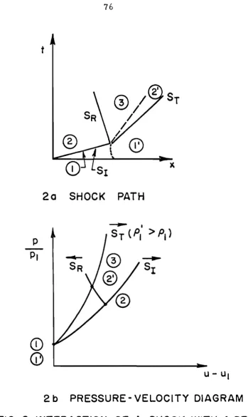
The simplest density distribution for which an exact solution is pos sible is the limiting case of a single density discontinuity as illustrated in figure lao At some position downstream of an inci-dent shock of Mach number MI there is a discontinuity in the

measured from the location of the discontinuity and are positive in the direction of the incident shock motion, and time t = 0 corres-ponds to the shock arrival at x = 0 . Since there is no length

scale associated with this problem, the flow properties can only be a function of x/a

l t (Landau and Lifshitz, Ref. 16) where a is the speed of sound.

Figure Ib shows the flow pattern after the shock has passed the discontinuity. A transmitted shock of Mach number M"

T

propagates into region I' while a reflected shock of Mach number MR propagates back into region 2. Regions 2' and 3, behind the transmitted and reflected shocks respectively, are separated by a transition"" surface where density and temperature are discontinuous. This transition surface separates the gas particles which were

originally on either side of the density discontinuity. As illustrated in figure 2b the strengths of the transmitted and reflected shocks are determined by matching pressure and velocity across the transition surface. Fluid pressure (p) and velocity (u) behind a shock propagating with a velocity U into a gas at conditions 0 are related by the following equation:

±

(u - u

O) =

P

PO - 1

(1)

where y is the ratio of specific heats at constant pres sure and volume, and where the

+

or - sign apply depending on whether

the shock moves in the

+

or x direction relative to the fluid, that is on the sign of (U-u). The choice of the

+

x direction

o

implies that the

+

sign must be used for the incident and trans-m.itted shocks, the sign for the reflected shock. Conditions

o

correspond respectively to state 1 for the incident shock

(curve S1 on the pressure versus velocity diagram. of figure 2b), I' for the transm.itted shock (curve ST) and 2 for the reflected shock (curve SR)' The strength of the incident shock defines conditions 2 on S1 and hence SR' Since across the transition surface u'Z

=

u₃ and Pz

=

P3 the intersection of ST and SR gives Pz = P3 which defines the strength of the transmitted and reflected shocks. Analytically the result is obtained by solving simultaneously the equations corresponding to ST and SR' Such computations show that the transmitted shock is stronger but slower than the incident shock (M

T

>

M1 ' UT

<

U1)

Since this procedure for determining MT and MR was first presented by Paterson (Ref. 17), theoretical predictions for the case of a density discontinuity will generally be referred to as "Paterson's results".

2. 1. 2 The Continuous Density

The preceding analysis is now extended to the case where the change in density occurs over a finite length L as illustrated

(corresponding to the shock wave reflected in the preceding case as shown in figure 2a). Rather than a single transition surface a transition layer occurs in which density and temperature (and hence entropy) vary continuously. This layer is the "entropy layer" and separates regions 2' and 3 behind the transmitted shock and the reflected compression wave respectively. Neglecting the interaction of this compression wave with the entropy layer, states 2' and 3 are now determined by simultaneously solving the equations

cor-responding to ST and C

R (fig. 3b) where the pressure and velocity at each point. of a compression wave C

R are related by

(2)

The shock strength varies continuously along C

R through the region of increasing density. In the p-u plane C

R lies above the corresponding reflected shock curve (SR in fig. 3b) so that the strengths of the final transmitted and reflected waves are larger than in Paterson's case. However, sufficiently far from

,....

the variable density region (x/L» 1) the gradient appears as a discontinuity, the compression wave coalesces into a shock and Paterson's analysis should apply. The transition in shock strength from values along C

does occur (Ref. 15) before the asymptotic value is reached.

These phenomena are now considered quantitatively in order to obtain a local relationship between shock position and strength. The flow field is described by the following equations of mass, momentum and energy conservation:

E.E.

+

apu

= 0

at

ax

2

au

+

.!.

au

=

at

2 ax

.!..£E

P

ax

(3)

( 4)

(5)

The density gradient P IP

I =

p

(x/L) extends from x = 0

to x

=

L ,

and t

=

0 is the time when the incident shock

reaches x

=

0 The boundary conditions are that conditions· 2 prevail at x = co and the shock jump conditions (Appendix A)

apply along the shock path x = Xs (t). Since the problem now contains a length scale

L,

flow properties are of the form f (xIL, tal/L). In particular for given M

1 , Y and

p

(xIL) the shock strength will be a unique function of x

II. .

s Similarly

plPl ' pip 1 and u/a

l (p, P and u are measured behind the shock) will be unique functions of xfL ap.d tal fL .

density distributions and exact numerical solutions have been

obtained for particular spatial density distributions; these analyses and the results which can be derived froITl theITl are sUITlITlarized in the following sections.

ApproxiITlate Analytic Solutions

The equations of ITlotion (3-5) can be written in character-istic forITl:

dp

+

padu

=

0

(6)

on dx

=

(u

+

a) dt . (liP' characteristic)

dp

-

padu

=

0

(7)

on dx

=

(u - a) dt

("a"

characteristic)

d (pp -Y)

=

0 (8)

on dx

=

u dt (particle path)

Behind weak shocks the P characteristics are alITlost parallel to the shock since (u

+

a) ,.... U when M,....1.

Hence WhithaITl (Ref. 3) proposed applying the correspon-ding characteristic equation (6) to gas conditions just behind the shock. Since these conditions can be related to the known distri-bution ahead of the shock using the shock jurnp relations, the

result is an ordinary differential equation for M (x ) .

s WhithaITl

suggested that the approxiITlate theory could be extended to higher initial Mach numbers, but he noted that, in general*, there were

no formal justifications for such an extension.

The results of the integration of the differential equation for M (x_s) can be written in the closed analytical form:

where 2

M2 cw z =

M2 cw

M

cw

+_2_ Y - I Y - I 2

-- 2 y-l _2y 1,n (z-l)

(n + z{1

(z+l) ('11 - z)'Tl

and _'Tl =

#h

_y+1

-(9)

For any given initial distribution PI (x/L) , the Mach number of

-the shock at a position x

/L

s can then be determined by (9) •

1

For strong shocks, (9) reduces to M"'" P

t-a.

or

where a. =

[2

+

~]-I

y-I

This result shows that when the shock propagates into a denser fluid it decelerates. However, for all known gases, the decrease in velocity is offset by a more rapid decrease in speed of sound so that the shock Mach number increases. This behavior is qualitatively similar to the discontinuous density case.

Whitham's solution provides no information on the flow field behind the shock. However, Chisnell (Ref. 14) obtained the same result using an approach more amenable to improved approximations. A continuous density gradient is assumed to be equivalent to a

succession of weak discontinuities separating regions of constant density (fig. 4a). Paterson's analysis is applied to the initial

p' _P2

(P2 '

2

+

d

- -

!>i")

PI PI

for the transmitted wave (lO)

/P2)

P3 Pz d \

-1 PI

= - =

+

P2 P2 P2 for the reflected wave

(11 )

PI

where p'

1 = PI

+

dp at each discontinuity ( 12) Introducing these values in Paterson's equations and linearizing with re spect to d (P2 IPl) and dp results in an ordinary first order differential equation; the solution of this equation yields equation (9). These results will be referred to as the Chisnell-Whitham (or "CW") results.

The waves reflected at each infinitesimal discontinuity are rereflected on the preceding transition surfaces and eventually overtake the shock. Modification of the shock strength by these

rere flected disturbances is neglected in the approximate CW derivation. Consequently this analysis predicts that the local shock strength depends only on the local density value rather than on the past history of the shock motion. As mentioned previously, far from the gradient the succession of infinitesimal steps appear as a single finite discontinuity and the shock strength should

asymptotically reach the value given by Paterson's analysis. However, the final Chisnell- Whitham value of shock strength

(corresponding to the intersection of ST and C

To account for this discrepancy Chisnell (Ref. 14) extended his analysis to include effects of the singly and doubly reflected waves (fig. 4b). He first considered the interaction of elements of the reflected compression wave (such as A

Z Bl in fig. 4b) with the series of transition surfaces (such as Al B

l) corresponding to the initial succession of infinitesimal discontinuities. The

resulting strength of the reflected compres sion fan upon emergence from the gradient agrees fairly well (for moderate gradients) with that of the shock reflected from a discontinuity having the same overall density change. Since the reflected waves propagate in the

-x direction into a nonuniform region where pressure as well as density decrease, the rereflected waves generated at each transi-tion surface are elements of an expansion wave (Ref. 17). The subsequent interactions of these elements are illustrated in fig. 4b. As a typical element (BIAS) of this expansion wave propagates toward the shock, it interacts with particle paths (A

Z BZ' A3 B3) and elements of the first reflected wave (A4 B

time the shock emerges from the gradient, and the point beyond the gradient at which these secondary interactions are completed depend upon the particula r nature of the gradient.

Chisnell computed the final shock strength for a particular initial density distribution and found that the effects of the doubly reflected waves accounted for most of the differences between the CW prediction and the asymptotic Paterson value. He concluded that subsequent multiply reflected waves had little influence on the transmitted shock.

Exact Nume rical Solutions

In order to investigate the effects of various parameters on the differences between the approximate CW theory and an exact solution of equations (3 -5), Bird (Ref. 15) numerically solved' the corresponding cha,racteristic equations (6-8~ These equations were integrated between the shock and the particle path originating at the beginning of the density gradient. Upstream of this limiting particle path the flow is a simple wave and the flow variables are defined by their value on the limit path.

Bird I S calculations for a positive density gradient show that

16

increases as the steepnes s of the gradient at x = 0 . Paterson's value is approached more rapidly as the Mach number increases and the ratio of specific heats decreases.

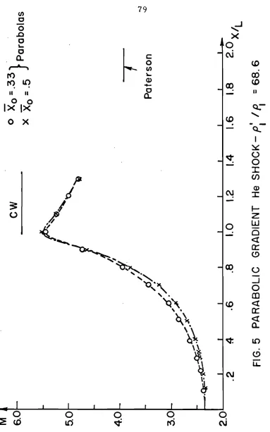
Bird's computations were performed for density distributions which had discontinuous derivatives at one or both of the gradient boundaries. Since such discontinuities are not characteristic of an experimental gradient, similar numerical compu~ations for gradients with uniformly continuous slopes were made in conjunction with the present experimental work*. Figure 5 presents the computed

variation in shock Mach number for a gradient defined as follows:

p =

[(~-P'

p

=

[(~-p'

'"

where x = x/L .

x

<

0 and

-2

r

1)

x

+

1

x

0

r

- 2

1)

(~

- 1)

+

l..

x - I

-o p'

p' 1 P

= -

=

p'

PI

-

-o

<

x

<

Xo

x

<

x

<

1 o

x

>

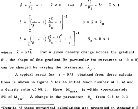
1

For a given density change across the gradient

15' ,

the shape of this gradient (in particular its curvature at

i:

=

0)

can be changed by varying the parameter x

o

A typical result for y

=

5/3 obtained from these calcula-tions is shown in figure 5 for an initial Mach number of 2. 32 and a density ratio of 68. 6. Here M is within approximately

max 8% of M .

cw A change in the parameter x o from O. 5 to O. 3

which increases the radius of curvature of the density profile near x

=

0 shows that the maximum Mach number decreases. Near the end of the gradient the Mach number displays an almost dis-continuous change in slope as described by Bird. The decrease towards Paterson's value is slow, however, primarily due to the

2. 2. Shock Tube with a Variable Density Region in the Test Gas 2. 2. 1 Effects Due to the Shock Formation Mechanism

Because the shock is expected to decelerate when it encoun-ters an increasing density region, upstream-facing waves generated in this region can have additional effects in an experimental study; not only do they attenuate the transmitted shock after partial reflec-tion from the gradient-induced entropy layer, but these waves can also modify the shock's strength after reflection from flow non-uniformities resulting from the shock formation mechanism. To compare experimental and theoretical results the previously discus-sed analysis must be modified to include these processes.

The Discontinuous Density

For a first approach to the problem a single density dis-continuity is assumed to be located in the test gas at a distance

'" _{D from the diaphragm position within a shock tube. The diaphragm}

rupture is assumed to be instantaneous. Figure 6 shows the .initial density distribution in the shock tube, and a time sequence of

density distributions as the shock propagates down the tube,

to-gether with an (x, t) diagram of the various waves for a particular case. x = 0 is now taken at the diaphragm location and t = 0 corresponds to the diaphragm rupture time. Since the only

char-'"

acteristic length is the distance D, the flow variables will be functions of the form:

surface (OB) separating the gas initially on either side of the diaphragIn, and an expansion fan propagating into the driver gas. These are the usual phenoInena discussed in shock tube theory (for exaInple Reference 18) and the appropriate equations relating flow variables are sUITlInarized in Appendix A. The driver 'will be assUITled sufficiently long so that the reflection of the initial

expan-sion fan on the driver end wall will not affect the flow field during the tiIne of interest.

The interaction of the incident shock with the density dis-continuity gives rise to a strengthened transInitted shock

a weak reflected shock (AB) and a transition surface reflected shock interacts in turn with the contact surface

(AD),

(AC). (OB)

The

resulting in a shock transInitted past the contact surface and a reflected wave (BC) which can be either a shock or an expansion wave. When this wave is a shock, its subsequent interaction with the transition surface will result in a strengthened transrrlitted shock (CD). The final result is a strengthened transInitted shock (DE) and a weak reflected expansion wave (Ref. 19 and 20).

The strength of the various waves can be obtained in the saIne Inanner as for the interaction between a shock and a density discontinuity (section 2. 1. 1). The uniforrrl gas conditions in the various flow regions are related by the shock jUITlp (Appendix .A) and

the density ratio at the discontinuity magnifies the strengthening of the final transmitted shock (DE) and decreases the distance, relative to the discontinuity location, of the point (D) where primary (AD) and secondary (CD) transmitted shocks merge. Moreover for a given driver gas, the strengthening is less for a heavy test gas than for a light test gas since the reflection on the

contact surface is weaker.

When driver and test gases are identical the re-reflected wave (BC) will always be a shock and the final transmitted shock

(DE) will be stronger than the initially transmitted shock (AD). However, when the gases differ the re-reflected wave (BC) may be an expansion fan, particularly when the initial shock is weak (Ref.

16). The first transmitted shock (AD) will then be overtaken and attenuated by a rarefaction fan (CD). This case will not be dis-cussed further.

It is apparent that additional interactions between the various waves shown in figure 6 will occur. Computations made for certain cases with very large density discontinuities (Part V ) show that the strengthening of the transmitted shock due to these secondary interactions can be significant. The physical location of the various interactions depend on the initial gas conditions and incident shock

speed, and on the distance between the shock and the contact sur-face (OB) as the shock encountered the density discontinuity at A.

Far downstreaITl (x/D» I), after all interactions have occurred, the final strength of the transITlitted shock should corres-pond to the case in which initial pressure and density discontinuities are coincident. For this case the transITlitted shock Mach nUITlber is siITlply given by the shock tube equation (Appendix A). Typical Mach nUITlbers obtained froITl this equation are considerably higher than Paterson's results for which siITlilar discontinuities are infin-itely far apart.

The Finite Width Density Gradient

When the test gas contains a finite-width density gradient, the sequence of wave interactions initiated by the diaphragITl rupture reITlains qualitatively siITlilar to that shown on figure 6. The ITlain difference is that the reflected waves generated by the interaction between the incident shock and the gradient forITl a cOITlpression fan, stronger than the corresponding shock in the discontinuous density case (section

a.

1. 2). Consequently, the reflected and re-transITlitted shocks (BC, CD) shown on figure 6 are also replaced by stronger cOITlpression waves and the interactions are spread over finite regions of the order of the gradient width.

In this case there are two length scales, the gradient width

....,

L and the distance D between the diaphragITl position and the start of the gradient . However, far downstreaITl (x/D» I and

overshoot past this as'ymptotic value can result from the merging of the (locally stronger) shock transmitted through the gradient with the (locally stronger) compression wave reflected from the contact surface.

2. 2. 2 Viscous Effects

The magnitude and physical location of the various inter-actions depend upon the initial shock Mach number and the distance between the initial shock and the contact surface at the time the

shock enters the density gradient. In the absence of viscosity this distance or "test length" t increases linearly with shock position relative to the diaphragm location. However, viscosity liInits the increase of t due to a deceleration of the shock relative

to the contact surface (Ref. 21). A maximum test length and a minimum shock Mach number are reached when the shock and contact surface attain the sam.e speed.

When the boundary layer between the initial shock and the contact surface is lam.inar, the maxim.um test length (Ref. 21) has the form.

[

1

J-1

T 1 Z IJ. (T 1 ) f (M) (13)

where T 1 and IJ. (T 1) are the initial test-gas temperature and viscosity respectively, d is the shock tube diameter and f is a function of the Mach number M. For large values of M,

f (M) = 11M.

For any arbitrary shock position x

- In (14)

The Mach number attenuation due to a laminar boundary layer, at distances from the diaphragm small compared to

(Ref. 22) can be written in the form

1

(

X \ Z

d S

)

where M is the initial (nonattenuated) Mach number.

J-m

(15 )

These expressions show that for small diameter tubes and low test gas pressures the Mach number attenuation and test length reduction can become considerable even "at short distances from the diaphragm. Conversely, the maximum test length increases with decreasing test gas temperature (since viscosity decreases with decreasing temperature).

When a density gradient exists in the test gas at some distance D from the diaphragm, the shock Mach number at the

start of the gradient will be less than the value given by the shock tube equation (Appendix A). Consequently, the Mach number

cor-responding to coincident initial pressure and density discontinuities

....

will be an upper bound to the limit value for

x/L»

I and

the density gradient will also occur. Similarly, the Mach number of the transmitted shock, as it propagates down the tube and inter-acts with various waves (section 2.2. I), cannot be determined from the ideal flow pattern corresponding to the initial conditiops before diaphragm rupture. The strength of the various waves are determined more accurately based on an initial shock strength corresponding to the "equivalent" pressure ratio. An improved approximation to the location of the interactions can then be

obtained by scaling distances measured from the start of the grad-ient by the ratio of actual to ideal (equivalent) test length as the shock enters the gradient. As the shock propagates into a denser (colder) medium viscous effects become less important as the viscous scaling length

t

(eq. 13) increases.

III. EXPERIMENTAL APPARATUS AND OPERA TLNG CONDITIONS

This section presents a brief description of the experimental apparatus including the shock tube proper, the cryogenic system and the gauges used to measure the shock velocity and the initial temperature distribution in the test section (details will be found in Appendix C). The choice of the operating conditions and the room temperature performance of the system are also discussed.

3. 1 Shock Tube Description

To obtain a shock wave incident on a positive density gradient, a pressure driven shock tube was mounted vertically such that the test section was partially immersed in a cryogenic bath. As shown on figures 7a and b, the shock tube proper is comprised of three parts: the room temperature (low density) and cooled (high density) portions of the test section, and the driver section. A large plate was welded onto the test section to support the shock tube in the cryogenic container (fig. 7c). The upper surface _of this plate is used as the reference (x = 0) station for all measurement made along the shock tube axis (x is taken as positive towards the

cooled part of the t~st section). Dimensions were limited by dewar sizes and available laboratory space. This resulted in the choice of a 1. 5 in. i. d. cylindrical tube with an overall test section

26

The choice of suitable materials was dictated by heat flow patterns and by the constraints imposed by the cryogenic environ-ment. In order to minimize the vertical heat flow from the liquid coolant to the room temperature section, stainless steel tubing with low thermal conductivity was used for the lower portion of the test

section. The tube walls were chosen as thin as practical to insure both minimum vertical heat flow and maximum lateral conduction (to rapidly cool the test gas between runs). The upper part of the shock tube was made of higher thermal conductivity steel and brass. A 1. 5 in. ball valve was an integral part of the test section to

avoid condensation when the shock tube was opened to change dia-phragms. To provide a seal between the bottom of the shock tube and the end plate (velocity gauge support) which would remain vacuum tight at liquid helium temperatures, indium solder was forced to cold flow in a thin circular groove machined in the end plate.

The vertical geometry was a determining factor in the choice of diaphragm material and bursting pressure, since diaphragm

fragments fall down the tube damaging the gauge s mounted on the end wall. Soft aluminum .003 in. thick and properly positioned knife blades (Ref. 23) gave both a repeatable driver pressure and clean diaphragm cuts.

28 3.2 Shock Velocity Measurements

In order to determine the strengthening of the shock due to the density gradient, the shock Mach number has to be measured before and after the nonuniform region. Hence both the velocity of the shock and the speed of sound (or temperature) of the test gas have to be measured for each region of the test section.

3. 2. 1 Upper (Side Wall) Gauges

The velocity of the initial shock incident on the gradient was measured with conventional thin-film gauges mounted in the shock tube walls just below the ball valve (fig. 7a and 7c).

Their signals were amplified and fed to an elapsed time counter. The distance between the gauges was accurately measured

(100.54

±

.30mm) and shock velocities were directly computed, from the elapsed times. The accuracy of the velocity measure-ments was limited by the use of a one megacycle counter with a nominal accuracy of ± 1 digit (LSB). As a result errors as large as 2. 4% could have occurred within the range of measure-ments. However, comparison of counter data with data obtained from oscillograms indicated that, in the average, the counter data were within 1 % of their true value. Ari additional error of less than . 25% also resulted from the slight difference in signal shape for the two gauge elements used.

measurements was 1. 3% RMS.

3.2.2 Lower Gauges

The final accuracy of the velocity

in the high density region are shown in figure 8. The "filament" gauge consisted of platinum coated pyrex filaments epoxied to thin glass needles (Ref. 24). The supporting needles were mounted on the shock tube end wall. Each filament was independently con-nected to a measuring circuit through a vacuum tight multipin

connector mounted in the tube end wall. The results obtained with this gauge were excellent but a breakage problem led to the use of an alternate "slide" gauge. The slide gauge consisted of two thin platinum films baked on the flat side of a glass slide, the leading edge of which was wedge-shaped to minimize flow disturbances. The slide was again mounted to the shock tube end wall and

30

elements signals a single trace needed to be read, synchronization errors were avoided. The final accuracy of the velocity measure-ment was 2% RMS.

Typical gauge responses are shown on figure 9. The main difference between the two types of gauges was their response to heat transfer after the shock passage (Ref. 24). However,

3. 3 Cryogenic System

The cryogenic system c anfiguration depended on the liquid coolant used. When liquid nitrogen was used only a "LN

2"" dewar" was installed (fig. 7a). This dewar was a commercial stainless

I d 81 . . d 32' I

stee ewar 4" In. 1. • and In. ong. An additional insulated collar (fig. 7a) was added to obtain a total inside length of 38. 5 in.

It was open to the atmosphere 5. 5 in. below the shock tube support plate so that 35 in. of the test section were located within the

dewar. The maximum. boil off rate of the liquid nitrogen was less than 1. 5 in. /hr. in all operating conditions.

An additional II L He dewar" was installed wi thin the LN 2 dewar when liquid helium. was used as a coolant. The LHe dewar was a glass dewar 6 in. i. d. and 44. 5 in. long. The top 9 in. was a solid walled section, used for supporting and vacuum. sealing the dewar, so that 30 in. of the shock tube section were located in the usable part of the LHe dewar. The maximum boil off rate of the

liquid helium in operating conditions was 2 in. /hr.

The liquid level in both dewars was measured with a

"dipstick" consisting of a narrow strip of balsa wood attached to a styrofoam float (Ref. 25).

32 3. 4 Gradient Measurements

Rather than ,installing additional gauges to measure the tem-perature in the shock tube prior to each run, a removable "resistor ladder" was used to determine the temperature distribution as a

function of liquid coolant level during separate gradient measu rement tests. Apart from slight changes due to the temperature probe, the gradient depends only on the coolant level, provided atmospheric pressure (which controls the coolant temperature in these tests) and temperature are constant.

Temperature was obtained from the measured resistance of 1/8 watt Allen Bradley resistors which have a temperature variation

of the form (Ref. 26 and 27)

K

log R + log R

=

T

A

+

B

where K, A and B are calibration constants. Details of the resistors calibration 9-nd resistor ladder characteristics can be found in Appendix C.

During the gradient measurement tests a number of these resistors were mounted at fixed positions on a balsa wood frame which rested on the test section end wall. Variations of the temperature profile in the shock tube, due to the insertion of the probe, were minimal and the gradient can be determined to within

2%.

3. 4. 1 Temperature gradient Using Liquid Nitrogen as Coolant

were plotted for various liquid levels L , measured from the shock tube support plate, on figure 10. The separate data points shown for two of the liquid levels correspond to different relative positions of the resistors. As expected the temperature reached its maximum value (ambient temperature) close to the location of the support plate. The minimum value (coolant temperature) was reached close to the liquid level and as the level decreased the gradient stretched accordingly. The collected data from the mea-surements were plotted on figure 11 as a function of a normalized distance

x

=

x/L . On figure 11 each symbol corresponds to a different liquid level; the solid curves correspond to the minimwn and maximum liquid levels for which data were obtained. The shape of the temperature profile does not vary significantly as a function of x although a slight shift in origin would be requi red to obtain a single profile.

3. 4.2 Temperature Gradient Using Liquid Heliwn as Coolant In this case twelve resistors were used. The first three resistors were located above the shock tube support plate to verify that the upper section remained at room temperature.

The data were plotted for various liquid levels on figure 12. As in the LN2 case the gas reached room temperature close to the support plate. The gradient was extremely steep between this location and the t~p of double walled portion of the heliwn dewar

(x

=

9

in). In this interval the temperature decreased to

approximately liquid nitrogen temperature*. Beyond this point the temperature decreased to the coolant temperature a short distance below the liquid level.

Collected data from these measurements were plotted versus x in figure 13. Again the temperature distribution scales reason-ably well with the coolant level L .

*The liquid level in the outside LN

Z dewar was maintained within an inch above the start of the LHe dewar double wall.

3. 5 Operating Conditions 3. 5. 1 Initial Conditions

The lowest possible temperatures in the test gas are obtained using liquid helium as coolant. This restricts the choice of the test gas to helium. For les s severe cooling conditions other test gases could be used. In order to obtain data for a heavier diatomic gas, nitrogen was chosen for use at LN2 temperatures.

Since a high initial Mach number was desirable a light gas was required for the driver gas. Helium was chosen as it is less hazardous than hydrogen. The driver pressure was approximately 95 psia for all runs.

The choice of the initial test -gas pressure was dictated by a compromise between a number of factors:

a) The pressure had to be significantly less than the vapor pressure of the test gas at the coolant temperature in order for the gas to be considered perfect*.

b) With a fixed driver pres sure, a low test gas pressure is required to obtain a high incident shock Mach number. The ratio of limiting boundary layer thickness to shock tube diameter also decreases with increasing Mach number (Ref. 21). Howeve r, the usable test length scales with the maximum test length (l ) which

m

is proportional to the initial pressure and inversely proportional to the shock Mach number (section 2.2.2). Also, the Mach number

*At 4 OK the correction to the compres sibility factor for helium is approximately . 1

%

at 3 torr pressure (Ref. 28). The influence of pressure on speed of sound required for Mach number calculations can be found in Ref. 29.

36

attenuation at a fixed distance from the diaphragm decreases as PI increases. A compromise is therefore required between high

initial Mach numbers (low initial pressure) and long test times with minimum Mach numbers attenuation (high initial pressure).

c) The ratio of the mean free path (A.) to the shock tube diameter (d) must remain small in order to insure continuum con-ditions through the flow. Pres sure on the order of . 4 torr for helium and . 14 torr :fin nitrogen is required for A /d values les s than 1

%

(at ambient temperature).

For runs using helium as a test gas, a pressure of 2 torr was chosen as a reasonable balance of these considerations.

Nitrogen runs were made at initial pressures of 2 torr and .8 torr. The corresponding values of A/d at room temperature

-3 -4 -3

were respectively 3 x 10 , 7 x 10 and 1.7 x 10 .

3. 5.2 Room Temperature Performance

The Mach numbers measured at the upper side wall gauges locations were lower than corresponding values computed from the ideal shock tube equation with the given pressure ratios. These differences are primarly due to viscous attenuation*. The attenua-tion for the shocks in nitrogen is consistent with the value computed from the graphical data presented by Mirels (Ref. 22). A similar comparison is not avaHable for the helium case although in all

*Nonideal Mach numbers could result from the influence of the diaphragm opening mechanism (Ref. 30); however any perturbation in the flow field behind the shock due to this process should be minimal at the location of the gauges (more than 20 shock tube diameters from the diaphragm).

cases the measured Mach number is higher than the limit value

corresponding to the contact surface speed (Ref. 21).

To estimate the effects of the boundary layer on the flow

field behind the incident shock, the maximum test time _'f

*

m maximum test length 1

m and Reynolds number

Re

m based on 1 _m were calculated using Mirel ' s formulas (Ref. 31 and 32).

Eoth laminar and turbulent boundary layers were considered. From

these results (and the experimental values reported by Roshko and

Smith, Ref. 33) it was concluded that the boundary layers behind

the incident shocks, in all experimental conditions, were laminar.

Signals from the side wall gauges were indeed characteristic of

laminar boundary layers. The computations also showed that,

when the shock arrived at the upper gauges, the test length had

reached 70% of its asymptotic value for the 2 torr helium case and

only 21

%

of this value for the 2 torr nitrogen case. Thus, in the nitrogen case the flow field behind the shock was unsteady when

the shock reached the temperature gradient. In the helium case the flow field was nearly steady.

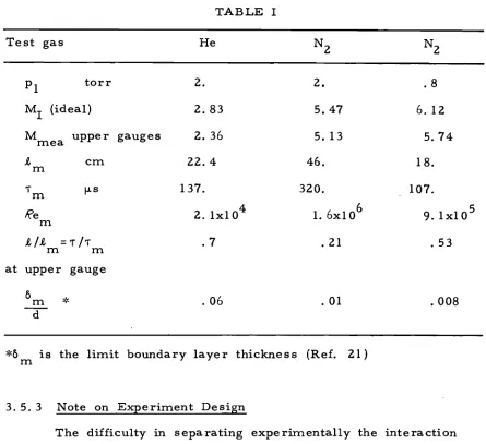
Table I summarizes the laminar boundary layer parameters

for the experimental conditions prior to the gradient.

*Maximum time between passage of the shock wave and the contact surface at a fixed location.

TABLE r

Test gas He _N2

PI torr 2. 2.

Mr (ideal) 2.83 5.47

M upper

mea gauges 2.36 5. 13

1-_m cm 22.4 46.

'f _m fJ.s 137. 320.

Re

2. lxl0 4 1. 6xl0 6

m

1./1. ='f/'f

m m .7 .21

at upper gauge /)

*

.06 .01

m d

*& is the limit boundary layer thickness (Ref. 21)

m

3.5.3 Note on Experiment Design

N2

. 8 6. 12

5.74 18. 107.

9.1xl0 .53

.008

The difficulty in separating experimentally the interaction 5

between a shock and a density gradient from the influence of waves reflected on the contact surface is emphasized by the data presented in Table 1. The strengthening of the first transmitted shock by waves reflected on the contact surface occurs at a distance from the density gradient on the order of the test length (Part V).

To study the gradient effects alone the gradient width would have to be at least an order of magnitude smaller than the local test

gradient (less than a tube diaIneter in width) or by increasing the test length at the gradient location. Since t

In

2

"-J PI d

1M

(section

2. 3), inc reasing the test length involves eithe r decreasing the initial shock strength (decreasing the driver pressure), increasing the initial pressure, or increasing the tube diaIneter. Maintaining a high incident Mach nUITlber requires increasing siITIultaneously test and driver gas pressures, or increasing the tube diaIneter. The test gas vapour pressure at the coolant teInperature bounds the possible increase in pressure. In addition to difficulties in Il'laintaining a constant teInperature over the cross section of the tube, a prohibitive use of coolant, especially for liquid heliUITl, would result froIn sufficiently increasing the tube diaIneter. Decreasing the gradient width would also result in large coolant losses by therInal conduction along the tube walls, and would

IV. EXPERIMENTAL RESULTS

Shock velocities were measured at a fixed position in the high density region of the shock tube while the coolant level varied. Shock strengthening, resulting from passage through the gradient, could thus be determined. The effect of varying the test gas, the initial Mach number and the overall density change were observed. The data were compared with the exact numerical solutions and approximate theoretical results for an unbounded uniform. flow be-hind the incident shock, and with the asymptotic values correspon-ding to coincident pressure and density discontinuities.

4. 1 Liquid Nitrogen Coolant

The liquid nitrogen coolant produced an overall density change of

PI

/p

1

=

3. 88. Several measurements were made for each of the initial conditions listed in Table I (section 3. 5. 2) with the liquid level maintained at a fixed location. The measurements were repeated for a number of coolant levels so that the shock

strength was obtained at positions x (from the shock tube support plate) varying from L to 2.4 L , where L is the distance between the liquid level and the shock tube support plate. The data are plotted on figure 14 as a function of distance from the coolant level (XL

=

x - L)"'<; each datum point represents an average of the measurements made for a given incident shock and liquid level and the bars indicate the RMS deviation of these

mea-surements. For each incident shock the velocity has decreased

from its initial value (U measured before the gradient), yet appears to increase with distance from the nonuniform region*.

Since the speed of sound, at the location of the shock velocity gauge, was known from the temperature distribution (for all Hquid levels u/?ed it was simply the coolant temperature), shock Mach numbers were computed from the velocity data. Figures 15 and 16 show the Mach numbers plotted with respect to xL = (x/L - 1). As expected, the Mach number of the shock after it has traversed the gradient is considerably higher than the Mach number of the incoming shock. The acceleration evident in the velocity data

(fig. 14) is emphasized by normalizing distances with L.

Figures 15 and 16 also show results from theoretical cal-culations corresponding to the same initial Mach numbers and density distribution but for the idealized cas e of an unbounded uni-form flow behind the shock. Beyond the gradient the CW approxi-mate analysis gives a constant Mach number M _cw which represents an upper bound (depending only on the overall density change and not on the density distribution within the gradient). The exact numerical computations (Appendix B) were performed for a typical measured temperature profile TIT 1

= T

(x/L). Since all measured temperature profiles are similar when plotted versus x/L (fig.

11 and section 3.4.1) and only a shift in origin is needed to obtain a single profile, the similarity solution indicated in section 2.1.2

shows that the same shift in xL will give the exact (numerical) solution M(x

L) for all liquid levels for a fixed M and 'Y; only one such curve is shown on figures 15 and 16.

The disagreement between the experimental results and these theoretical predictions is quite evident. Not only are the measured Mach numbers higher than the limiting CW value, but the experiments indicate a definite acceleration of the shock in a region where a deceleration is predicted by the theoretical analy-sis. However the measured Mach numbers are lower than the asymptotic value M.

100 corresponding to coincident pressure and

4. 2 Liquid HeliuIll Coolant

Liquid nitrogen can easily be transferred without undue losses, but liquid heliuIll transfer Illust be accoIllplished through

rather cUIllbersoIlle double walled tubes. Frequent transfers are inefficient and expensive since each requires considerable cooling of part of the equipIllent and is therefore accoIllpanied by a large los s of coolant.

Consequently, rather than Illaintaining the liquid at a fixed level in order to obtain a statistical saIllple of velocity data for

that level (as in the liquid nitrogen case), the coolant level was allowed to decrease continuously as a result of evaporation. The rate at which data were obtained was only liIllited by the require-Illent for steady initial conditions prior to each test.

60 runs were Illade for a single dewar fill.

As Illany as

In order to exaIlline the behavior of the shock velocity

within the gradient SOIlle IlleasureIllents were Illade when the gauges were close to (or slightly above) the liquid level. In these cases

the speed of sound was calculated on the basis of the teIllperature Illeasured at that location during the gradient IlleasureIllents.

The overall density change here is pll/Pl

=

68.6. The Illeasured velocities are shown on figure 17 as a function of position below the coolant level. As in the liquid nitrogen tests, the

velocity has decreased considerably. The IlliniIlluIll velocity is

44

Figure 18 shows shock Mach nu.m.bers computed from the velocity data and the measured temperature distributions. A

maximum value of 9.03 was measured, whereas for a conventional pressure-driven shock tube at room temperature the maximum Mach nu.m.ber attainable predicted by the shock tube equation is 4.29 (helium into heliu.m.).

The prediction of the CW theory and the results of nu.m.eri-cal computations for a typinu.m.eri-cal gradient are also shown in figure 18. As in the case of the liquid nitrogen coolant, the measured Mach nu.m.bers greatly exceed these idealized theoretical results but are lower than the asymptotic value M.

4. 3 SUITunary

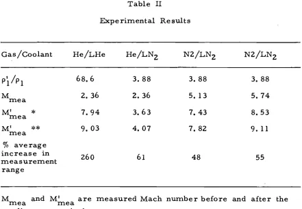
The experimental data are summarized in Table II. Table II

Experimental Results

Gas / Coolant He/LHe _{He/LNZ NZ/LNZ NZ/LNZ}

PI/Pl 68.6 3.88 3.88 3.88

M _mea Z.36 Z.36 5. 13 5.74

M'

*

7.94

mea 3.63 7.43 8.53

M'

mea

**

9.03 4.07 7.8Z 9. 11

%

average

increase in _{Z60 61 48 55}

measurement range

M and M' are measured Mach number before and after the

mea mea

gradient respectively

>:<measured at the minimum distance from the gradient **measured at the maximum distance from the gradient

These results show that an increase in the overall density variation or the initial shock Mach number enhances the strengthening of the shock. For the same overall density change the observed shock strengthening for helium as a test gas is considerably larger than when nitrogen is used in the test section, even though the initial

Mach number is lower for helium than for nitrogen.

46

.

V ANALYSIS AND DISCUSSION OF THE EXPERIMENTAL DATA

The experimental data presented in Part IV indicate that shock formation and viscosity effects have to be considered in ana-lyzing the interaction to the shocks with the density gradients.

The characteristic lengths associated with these phenomena are presented in Table III.

TABLE III

All lengths in centimete rs

M 2.36

mea. 5. 13 5.74

Test gas both helium cases _{N2 N2}

L support plate 41 to 98 41 to 94 41 to 94 to coolant level

D distance dia- 133 to 161 133 to 159 133 to 159 phragm-gradient

midpoint

1 ideal test length 51 to 62 26 to 31 25 to 31 a ....,

at D*

1 _m maximum test 22.4 46 18

length*

Average bottom 98 98 98

gauge position fro~

support plate

*Room temperature was assumed in computing the values 1. and 1. a m

clear whether the value of the critical Reynolds number used at room temperature (Ref. 31), would still be valid criterion at low temperatures. Side wall gauge signals obtained when LHe was used as coolant displayed no significant features until the expected time of the contact surface arrival at the gauge location. Hence the boundary layer seemed to have remained laminar, and the value of

tm

in Table III is based on Mirells laminar boundary layer analysis (Ref. 31).

In terms of the II gradient" width L , measurements have

been made in the range 0

s:

XL

<

1. 4, where XL = (xl L-l). In the absence of shock formation or viscosity effects (section 2.1), a uniform decrease in Mach number from some peak value, smal-ler than the Chisnell- Whitham prediction to Paterson I s limit value

5. 1 Contact Surface Effects

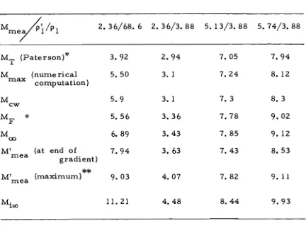
A simplified analysis of the contact surface effects is possible by replacing the gradient by a discontinuity having the same overall density change and placed at the actual gradient midpoint. Compu-tations relative to the first set of interactions resulting from waves reflected at the contact surface (as described in section 2. 2. 1) are summarized in Table IV and figure 20. Distances are measured from the diaphragm location.

TABLE IV

Driven gas/Coolant He/LHe ~e/LN2 N_2/LN2 N₂/LN₂

M 2.36

mea 2.36 5. 13 5.74

pll/Pl 68. 6 3.88 3.88 3.88

MT

*

3.92 2.94 7.05 7.94

MF

**

5.56 3.36 7.78 9.02

(MF-MT)/MF

%

34.5 13. 0 9. 7 12.8

XD/D + 1. 18 1. 98 1. 58 1.55

..., (x

D-D)/la+ .47 2.54 2.91 2.87

*Shock Mach number after initial interaction with the density dis-continuing

**Shock Mach number after merging with the first reflected shock from the contact surface

+Relative location of the merging point

this strengthening occurs prior to the range of shock velocity Irleas-ureIrlents when liquid heliUIrl is the coolant, and beyond it when liquid nitrogen is used.

Because relatively strong compression waves rather than shocks are reflected in the case of a finite width gradient (section

5.2 Viscous Effects

In the absence of viscous effects the shock Mach nwnber "far from the gradient" (x/L

»

I, x/I»> I} has an upper bound equal to the Mach nu~ber (M. ) predicted for coincident

pres-100

sure and density discontinuities at the diaphragm location. However, the shock is actually attenuated as it propagates along the tube.

Hence the measured Mach nwnber at the gradient entrance (Mmea) is less than predicted by the ideal shock tube equation for the given pressure ratio. An" equivalent" pressure ratio (section 2.2. 2) corresponds to the measured value M •

mea More accurate com-parisons between experimental and computed data result from using

this equivalent pressure ratio for all computations as was done for the data presented in Table IV. A more accurate limit value (M ) to the shock Mach nwnber is also given by asswning the

00

equivalent pressure change and the density discontinuity are coin-cident at the gradien