STRUCTURAL DAMAGE EVALUATION: THEORY AND
APPLICATIONS TO EARTHQUAKE ENGINEERING
Thesis by
Rustem Shaikhutdinov
In Partial Fulfillment of the Requirements
for the Degree of
Doctor of Philosophy
Report No. EERL 2004-06
California Institute of Technology
Pasadena, California
2004
© 2004
Acknowledgments
My sincere gratitude goes to my adviser Professor James L. Beck for his direction and encouragement throughout the course of this investigation. Without his invaluable guidance and support, this thesis would not have been possible. I am also truly grateful to Keith A. Porter for the suggestions and input that were most helpful. I am thankful for the delightful time we spent working together.
I truly appreciate the time and input of Professors Wilfred D. Iwan, John F. Hall in reviewing my thesis and delegating their time to serve on my thesis examination committee. It has been a really enriching experience to be their student, as well.
My studies were financially supported by funds from California Institute of Technology; California Universities for Research in Earthquake Engineering under the CUREe-Kajima joint research program, Phase IV; the Earthquake Engineering Research Centers Program of the National Science Foundation under Award Number EEC-9701568 through the Pacific Earthquake Engineering Research Center (PEER). These supports are gratefully acknowledged. Any opinions, findings and conclusions or recommendations expressed in this material are those of the authors and do not necessarily reflect those of the support providers.
I am thankful to Carolina Oseguera and Connie Yehle for always being so thoughtful and supportive throughout all the years of my staying at Caltech.
Abstract
Table of contents
1 Introduction... 1
2 Methods and challenges of performance-based earthquake engineering ... 7
2.1 Decision making for a real estate owner... 7
2.2 Methods of performance-based earthquake engineering ... 10
2.2.1 Overview of structural reliability theory for seismic safety ... 11
2.2.2 Performance-based earthquake engineering framing equation... 13
2.2.2.1 Standard integral form for arbitrary decision variables ... 13
2.2.2.2 Evaluation of damage and decision variables... 15
2.2.2.3 Performance-based earthquake engineering framing equation... 18
2.2.2.4 Fragility functions in PBEE framework ... 23
2.3 Challenges of PBEE design ... 24
3 Theory of fragility functions... 31
3.1 Single damage state... 31
3.1.1 Fragility functions of the structural members... 36
3.2 Multiple damage states ... 43
3.2.1 Fragility functions (not mutually exclusive damage states) ... 48
3.2.2 Selecting damage states ... 49
4 Damage estimation coupled with structural analysis (single damage state)... 53
4.1 EDP dependent on damage ... 53
4.1.1 Methods of damage estimation ... 53
4.1.2 Structural model description... 58
4.1.3 Damage model ... 60
4.1.4 Interpretation of the chosen damage model ... 64
4.1.5 Parameters of the damage model and ground motions ... 65
4.1.6 Results and conclusions ... 67
4.2 Inexact damage state description (imperfect limit-state function)... 80
4.2.1 Structural model... 82
4.2.2 Damage model ... 83
4.2.4 Results and conclusions ... 89
4.2.5 Alternative damage models for uncoupled damage analysis... 98
4.2.5.1 Utilizing additional information about components ... 98
4.2.5.2 Utilizing multidimensional fragility functions... 106
5 Damage estimation coupled with structural analysis (multiple damage states) ... 111
5.1 Structural model... 111
5.2 Damage model ... 112
5.3 Repair cost ... 115
5.4 Results... 116
6 Combined methods of damage estimation... 153
6.1 Example of application ... 153
6.2 Damage states of reinforced concrete members ... 158
7 The use of in-situ information for fragility functions ... 161
7.1 Generic fragility function (no in-situ information included) ... 162
7.2 Fragility function with in-situ information included ... 164
7.3 Results and conclusions ... 170
8 Conclusions and future research ... 177
9 References... 181
Appendix A. Probabilistic relation between damage states and repair methods. ... 189
A.1 Available repair methods ... 189
A.2 Statistics of application of repair techniques ... 194
Table of Figures
Figure 2.1 Example of utility function for decision making based on safety. 7 Figure 2.2 Example of a decision making process for a real estate owner. 10 Figure 2.3 Implementation structure of the PEER PBEE framing equation. 22 Figure 3.1 Fragility functions for multiple damage states 47 Figure 3.2 Damage states probability space for different values of EDP 47 Figure 3.3 Original state space and redefined state space with corresponding probability
measures 51 Figure 4.1 Relations between the variables in the state space. 53
Figure 4.2 Uncoupled structural and damage analyses. 54
Figure 4.3 Coupled structural and damage analyses 55
Figure 4.4 Methods used for the sample case study damage estimation. 57 Figure 4.5. Reinforced concrete moment-resisting frame chosen for the case study. 59 Figure 4.6. Flexural members hysteretic rule: Q-HYST. 60 Figure 4.7 Relation between force-displacement history and observed damage states of a reinforced concrete column (Tanaka and Park, 1990) 65 Figure 4.8. Expectation of damage E[Nt] as a function of spectral acceleration, ground
motion LA15. 73
Figure 4.9. Relative errors of estimation of E[Nt] by different methods as a function of
spectral acceleration, ground motion LA15. 73
Figure 4.10. Variance of the damage estimate as a function of spectral acceleration,
ground motion LA15. 74
Figure 4.11. Coefficient of variation of the damage estimate as a function of spectral
acceleration, ground motion LA15. 74
Figure 4.12. Expectation of damage E[Nt] as a function of spectral acceleration, set of
ground motion records. 76
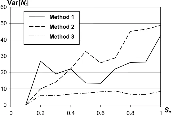
Figure 4.13. Relative errors of estimation of E[Nt] by different methods as a function of spectral acceleration, set of ground motion records. 77 Figure 4.14. Variance of damage estimation as a function of spectral acceleration, set of
Figure 4.15. Coefficient of variation of the damage estimate as a function of spectral
acceleration, set of ground motion records. 78
Figure 4.16 Example of the yield surface of the flexural members (axial force - moment
interaction). 83 Figure 4.17. Expectation of damage E[Nt] as a function of spectral acceleration for the
axial force-flexure interaction model, ground motion LA15. 92 Figure 4.18. Relative errors of estimation of E[Nt] by different methods as a function of spectral acceleration for the axial force-flexure interaction model, ground motion
LA15. 92 Figure 4.19. Variance of damage estimation as a function of spectral acceleration for the
axial force-flexure interaction model, ground motion LA15. 93 Figure 4.20. Coefficient of variation of the damage estimate as a function of spectral
acceleration for the axial force-flexure interaction model, ground motion LA15. 93 Figure 4.21. Expectation of damage E[Nt] as a function of spectral acceleration for the axial force-flexure interaction model, set of ground motion records. 94 Figure 4.22. Relative errors of estimation of E[Nt] by different methods as a function of spectral acceleration for the axial force-flexure interaction model, set of ground
motion records. 94
Figure 4.23. Variance of damage estimation as a function of spectral acceleration for the axial force-flexure interaction model, set of ground motion records. 95 Figure 4.24. Coefficient of variation of the damage estimate as a function of spectral
acceleration for the axial force-flexure interaction model, set of ground motion
records. 95 Figure 4.25 Safety regions for exact (hatched) and approximate (shaded) limit-state
functions, fragility function is CDF of capacity at zero axial force 99 Figure 4.26 Using flexural member's yield surface for determining safety region in terms
of yield moment at zero axial force 100
Figure 4.27 Comparison of the safety regions defined by exact and approximate limit-state functions for the assumed probability distribution of current axial force. 103 Figure 4.28 Safety regions for exact (hatched) and approximate (shaded) limit-state
Figure 4.29 Safety regions for exact and approximate limit-state functions, lower values of axial force expected value and standard deviation are used 105 Figure 4.30 Safety regions for exact (hatched) limit-state function and two-dimensional
approximate (shaded) limit-state function, axial force is relatively small 108 Figure 4.31 Procedure of finding safety region for two dimensional fragility function,
axial force is relatively high 108
Figure 4.32 Safety regions for exact (hatched) limit-state function and two-dimensional approximate (shaded) limit-state function, axial force relatively large 109 Figure 5.1 Hysteretic rule for flexural members (Q-HYST with strength degradation). 112 Figure 5.2 Expected number of flexural members in three damage states of interest,
obtained by Method 1, correlation of capacities 0.6, ground motion LA15. 120 Figure 5.3 Expected number of flexural members in three damage states of interest,
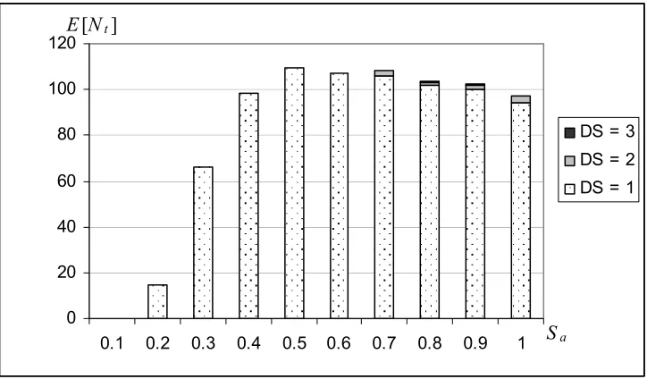
obtained by Method 2, correlation of capacities 0.6, ground motion LA15. 121 Figure 5.4 Expected number of flexural members in three damage states of interest,
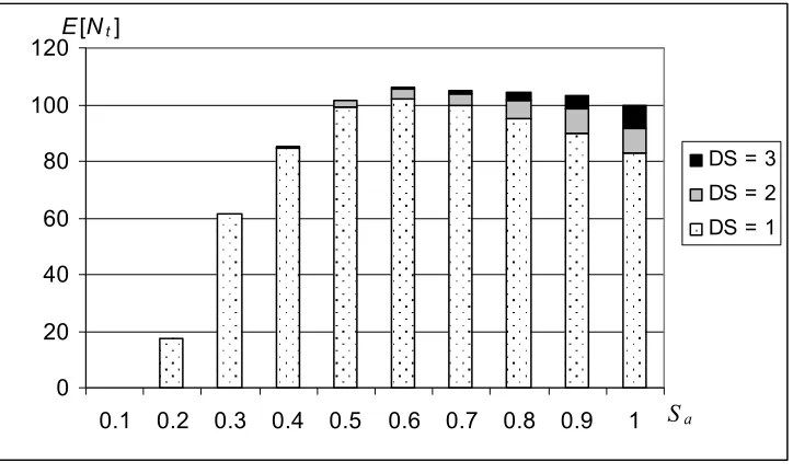
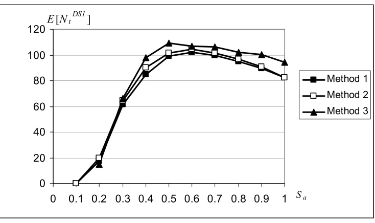
obtained by Method 3, correlation of capacities 0.6, ground motion LA15. 121 Figure 5.5 Expected number of flexural members in DS = 1 for multiple damage states model with correlation of capacities 0.6, ground motion LA15. 122 Figure 5.6 Expected number of flexural members in DS = 2 for multiple damage states
model with correlation of capacities 0.6, ground motion LA15. 122 Figure 5.7 Expected number of flexural members in DS = 3 for multiple damage states
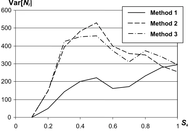
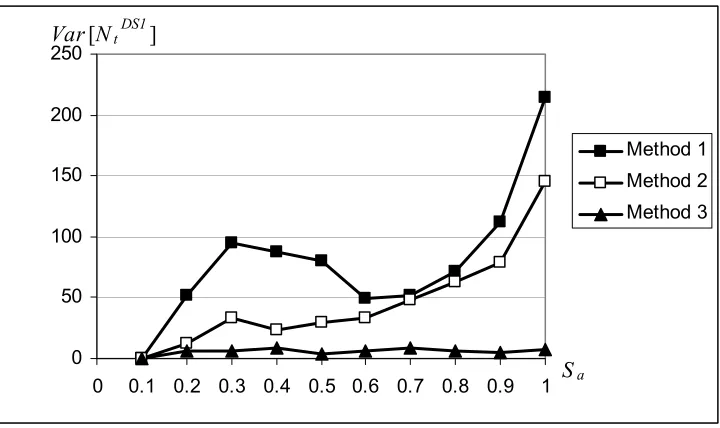
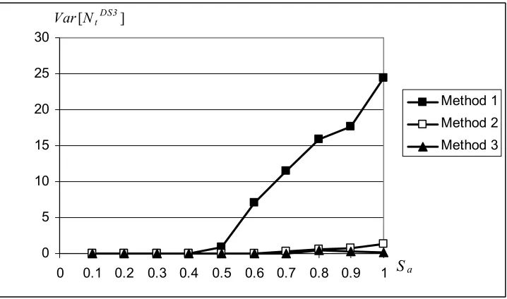
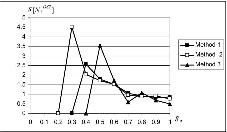
model with correlation of capacities 0.6, ground motion LA15. 123 Figure 5.8 Variance of number of flexural members in DS = 1 for multiple damage states model with correlation of capacities 0.6, ground motion LA15. 123 Figure 5.9 Variance of number of flexural members in DS = 2 for multiple damage states model with correlation of capacities 0.6, ground motion LA15. 124 Figure 5.10 Variance of number of flexural members in DS = 3 for multiple damage
states model with correlation of capacities 0.6, ground motion LA15. 124 Figure 5.11 Coefficient of variation of number of flexural members in DS = 1 for
multiple damage states model with correlation of capacities 0.6, ground motion
Figure 5.12 Coefficient of variation of number of flexural members in DS = 2 for multiple damage states model with correlation of capacities 0.6, ground motion
LA15. 125 Figure 5.13 Coefficient of variation of number of flexural members in DS = 3 for
multiple damage states model with correlation of capacities 0.6, ground motion
LA15. 126 Figure 5.14 Expected repair cost estimate for multiple damage states model with
correlation of capacities 0.6, ground motion LA15. 126 Figure 5.15 Variance of repair cost estimate for multiple damage states model with
correlation of capacities 0.6, ground motion LA15. 127 Figure 5.16 Coefficient of variation of repair cost estimate for multiple damage states
model with correlation of capacities 0.6, ground motion LA15. 127 Figure 5.17 Expected number of flexural members in three damage states of interest,
obtained by Method 1, correlation of capacities 0.6, set of ground motion records. 128 Figure 5.18 Expected number of flexural members in three damage states of interest,
obtained by Method 2, correlation of capacities 0.6, set of ground motion records. 128 Figure 5.19 Expected number of flexural members in three damage states of interest,
obtained by Method 3, correlation of capacities 0.6, set of ground motion records. 129 Figure 5.20 Expected number of flexural members in DS = 1 for multiple damage states model with correlation of capacities 0.6, set of ground motion records. 129 Figure 5.21 Expected number of flexural members in DS = 2 for multiple damage states model with correlation of capacities 0.6, set of ground motion records. 130 Figure 5.22 Expected number of flexural members in DS = 3 for multiple damage states model with correlation of capacities 0.6, set of ground motion records. 130 Figure 5.23 Variance of number of flexural members in DS = 1 for multiple damage
states model with correlation of capacities 0.6, set of ground motion records. 131 Figure 5.24 Variance of number of flexural members in DS = 2 for multiple damage
Figure 5.25 Variance of number of flexural members in DS = 3 for multiple damage states model with correlation of capacities 0.6, set of ground motion records. 132 Figure 5.26 Coefficient of variation of number of flexural members in DS = 1 for
multiple damage states model with correlation of capacities 0.6, set of ground
motion records. 132
Figure 5.27 Coefficient of variation of number of flexural members in DS = 2 for multiple damage states model with correlation of capacities 0.6, set of ground
motion records. 133
Figure 5.28 Coefficient of variation of number of flexural members in DS = 3 for multiple damage states model with correlation of capacities 0.6, set of ground
motion records. 133
Figure 5.29 Expected repair cost estimate for multiple damage states model with correlation of capacities 0.6, set of ground motion records. 134 Figure 5.30 Variance of repair cost estimate for multiple damage states model with
correlation of capacities 0.6, set of ground motion records. 134 Figure 5.31 Coefficient of variation of repair cost estimate for multiple damage states
model with correlation of capacities 0.6, set of ground motion records. 135 Figure 5.32 Expected number of flexural members in DS = 1 obtained by Method 1 for low (0.6) and high (0.9) coefficient of correlation of member capacities, ground
motion LA15. 135
Figure 5.33 Expected number of flexural members in DS = 2 obtained by Method 1 for low (0.6) and high (0.9) coefficient of correlation of member capacities, ground
motion LA15. 136
Figure 5.34 Expected number of flexural members in DS = 3 obtained by Method 1 for low (0.6) and high (0.9) coefficient of correlation of member capacities, ground
motion LA15. 136
Figure 5.35 Expected number of flexural members in DS = 1 obtained by Method 2 for low (0.6) and high (0.9) coefficient of correlation of member capacities, ground
Figure 5.36 Expected number of flexural members in DS = 2 obtained by Method 2 for low (0.6) and high (0.9) coefficient of correlation of member capacities, ground
motion LA15. 137
Figure 5.37 Expected number of flexural members in DS = 3 obtained by Method 2 for low (0.6) and high (0.9) coefficient of correlation of member capacities, ground
motion LA15. 138
Figure 5.38 Variance of number of flexural members in DS = 1 obtained by Method 1 for low (0.6) and high (0.9) coefficient of correlation of member capacities, ground
motion LA15. 138
Figure 5.39 Variance of number of flexural members in DS = 2 obtained by Method 1 for low (0.6) and high (0.9) coefficient of correlation of member capacities, ground
motion LA15. 139
Figure 5.40 Variance of number of flexural members in DS = 3 obtained by Method 1 for low (0.6) and high (0.9) coefficient of correlation of member capacities, ground
motion LA15. 139
Figure 5.41 Variance of number of flexural members in DS = 1 obtained by Method 2 for low (0.6) and high (0.9) coefficient of correlation of member capacities, ground
motion LA15. 140
Figure 5.42 Variance of number of flexural members in DS = 2 obtained by Method 2 for low (0.6) and high (0.9) coefficient of correlation of member capacities, ground
motion LA15. 140
Figure 5.43 Variance of number of flexural members in DS = 3 obtained by Method 2 for low (0.6) and high (0.9) coefficient of correlation of member capacities, ground
motion LA15. 141
Figure 5.44 Expected repair cost obtained by Method 1 for low (0.6) and high (0.9) coefficient of correlation of member capacities, ground motion LA15. 141 Figure 5.45 Expected repair cost obtained by Method 2 for low (0.6) and high (0.9)
coefficient of correlation of member capacities, ground motion LA15. 142 Figure 5.46 Variance of repair cost obtained by Method 1 for low (0.6) and high (0.9)
Figure 5.47 Variance of repair cost obtained by Method 2 for low (0.6) and high (0.9) coefficient of correlation of member capacities, ground motion LA15. 143 Figure 5.48 Expected number of flexural members in DS = 1 obtained by Method 1 for low (0.6) and high (0.9) coefficient of correlation of member capacities, set of
ground motion records. 143
Figure 5.49 Expected number of flexural members in DS = 2 obtained by Method 1 for low (0.6) and high (0.9) coefficient of correlation of member capacities, set of
ground motion records. 144
Figure 5.50 Expected number of flexural members in DS = 3 obtained by Method 1 for low (0.6) and high (0.9) coefficient of correlation of member capacities, set of
ground motion records. 144
Figure 5.51 Expected number of flexural members in DS = 1 obtained by Method 2 for low (0.6) and high (0.9) coefficient of correlation of member capacities, set of
ground motion records. 145
Figure 5.52 Expected number of flexural members in DS = 2 obtained by Method 2 for low (0.6) and high (0.9) coefficient of correlation of member capacities, set of
ground motion records. 145
Figure 5.53 Expected number of flexural members in DS = 3 obtained by Method 2 for low (0.6) and high (0.9) coefficient of correlation of member capacities, set of
ground motion records. 146
Figure 5.54 Variance of number of flexural members in DS = 1 obtained by Method 1 for low (0.6) and high (0.9) coefficient of correlation of member capacities, set of
ground motion records. 146
Figure 5.55 Variance of number of flexural members in DS = 2 obtained by Method 1 for low (0.6) and high (0.9) coefficient of correlation of member capacities, set of
ground motion records. 147
Figure 5.56 Variance of number of flexural members in DS = 3 obtained by Method 1 for low (0.6) and high (0.9) coefficient of correlation of member capacities, set of
Figure 5.57 Variance of number of flexural members in DS = 1 obtained by Method 2 for low (0.6) and high (0.9) coefficient of correlation of member capacities, set of
ground motion records. 148
Figure 5.58 Variance of number of flexural members in DS = 2 obtained by Method 2 for low (0.6) and high (0.9) coefficient of correlation of member capacities, set of
ground motion records. 148
Figure 5.59 Variance of number of flexural members in DS = 3 obtained by Method 2 for low (0.6) and high (0.9) coefficient of correlation of member capacities, set of
ground motion records. 149
Figure 5.60 Expected repair cost obtained by Method 1 for low (0.6) and high (0.9) coefficient of correlation of member capacities, set of ground motion records. 149 Figure 5.61 Expected repair cost obtained by Method 2 for low (0.6) and high (0.9)
coefficient of correlation of member capacities, set of ground motion records. 150 Figure 5.62 Variance of repair cost obtained by Method 1 for low (0.6) and high (0.9)
coefficient of correlation of member capacities, set of ground motion records. 150 Figure 5.63 Variance of repair cost obtained by Method 2 for low (0.6) and high (0.9)
coefficient of correlation of member capacities, set of ground motion records. 151 Figure 6.1 Repair cost estimates based on combined method of damage analysis, set of
ground motion records. 156
Figure 6.2 Expectation of repair cost estimate and one-sigma confidence intervals obtained by combined method of damage analysis, set of ground motion records. 157 Figure 6.3 Standard deviation of repair cost estimate obtained by combined method of
damage analysis, set of ground motion records. 157
Figure 7.1 Column model 161
Figure 7.2. Force-deformation characteristics of the shear spring (left) and flexural
spring (right). 162
Figure 7.3 Failure region and safe region in the Ω space. 164 Figure 7.4 Surface Ωz for different values of IDR 166
Figure 7.5 Surface Ωz for different values of α 166
Figure 7.6 Site-specific fragility function and CDF of capacity for the "normal strength"
Figure 7.7 Site-specific fragility functions for “normal strength” design for different
values of α 172
Figure 7.8 Site-specific fragility function and CDF of capacity for the "over-strength"
design. 174 Figure 7.9 Site-specific fragility functions for “over-strength” design for different values
of α 174
Figure 7.10 Site-specific fragility function and CDF of capacity for the "under-strength"
design. 175 Figure 7.11 Site-specific fragility functions for “over-strength” design for different values
of α 175
1 Introduction
The primary focus of the present study is structural damage estimation. Damage estimation is a vital part of the seismic performance evaluation of buildings and other structures with respect to multiple performance objectives. In turn, the proper evaluation of seismic performance is essential for decision making involved in managing the risk to building, bridges, and other infrastructure in seismically active areas. Today, the earthquake engineering community faces new challenges that are brought about by the latest needs of the real estate development and management industries. The safety of buildings and other structures used to be the main concern of designers, owners, and regulators. The development of modern building codes has provided society with guidelines that serve well for achieving the required safety levels. However, nowadays other issues are becoming significant for owners and risk managers. Providing that safety requirements are met, the questions being asked now are “how much does it cost to repair?”, “how long it will be shut down in case of the earthquake?”, etc. These questions relate to the economic aspect of the seismic performance of real estate. Given the multiple performance objectives, accurate damage estimation becomes more important than ever. The issues involved in the decision-making process with respect to various performance objectives and the role of damage estimation in this process are discussed in detail in Sections 2.1 and 2.2, respectively.
that are specified by some formal feature and/or parameters. For example, such classes may be: reinforced-concrete shear-wall building higher than 7 stories, or single-span bridge with monolithic abutment. Then a performance prediction model is built on the observed seismic performance of all available samples within the category. This approach is used, among others, by Hart and Srinivasan (1994) and by Basoz and Kiremidjian (1999).
More advanced techniques include specific building information in the damage analysis, such as particular design features and the site seismic hazard. The information about structural design is usually included in a finite element structural model. The structural model is used for carrying out a structural analysis. Damage analysis is then executed based on the results of the structural analysis. If better performance prediction is desired by the decision maker, then more site-specific information can be incorporated in the structural analysis and the analysis can be closer to the real-life behavior of the structure. For a relatively rough analysis, a simplified building model, like a shear beam, can be used in a pushover analysis. If more accurate results are desired, then more sophisticated structural models should be used, such as detailed finite-element models together with dynamic time-history simulation. Accordingly, the damage estimation technique should match the accuracy of the structural analysis.
performance of the advanced structural analysis tools, making these advances largely wasted for loss estimation studies. Indeed, since the seismic performance assessment is based both on structural analysis and damage analysis, the inaccurate damage evaluation prevents reliable performance estimation from being achieved. The highly accurate structural analysis will not contribute to the final goal – accurate performance estimation, because the structural analysis results will be diluted by the larger errors at the stage of the damage estimation. Thus, the goal here is to develop improved methods of damage estimation that are capable of providing the results with an accuracy that matches the accuracy of the most sophisticated structural models.
Before we proceed with the introduction to the different damage estimation approaches, we want to point out that increasing utilization of site-specific information in the seismic performance analysis can lead to a potential problem, related to the inherent difficulty of experimental verification of the site-specific analysis results. A more detailed discussion of this problem is given in Section 2.3. Another problem of seismic performance evaluation that can arise is due to the different sensitivity of the decision-making process to the errors in performance assessment for different decision criteria. The issues relevant to this problem are also considered in Section 2.3
At the present time, the common tools of general purpose damage analysis are fragility functions that are used for uncoupled damage analysis. These functions establish a probabilistic relation between structural response to seismic loading and the resulting damage to individual components. Historically, fragility functions were developed within nuclear engineering to evaluate the seismic resistance of nuclear reactors with respect to operational or safety failure. Later, their area of application was extended to other fields, such as estimation of the seismic resistance of electrical equipment or the seismic performance of civil engineering structures such as bridges and buildings. For all these applications, fragility functions proved to be convenient, versatile and reasonably accurate tools of damage estimation.
fragility function) can be spectral acceleration Sa, inter-story drift ratio (IDR), ductility demand, peak ground acceleration (PGA), etc., with the latter having been most heavily utilized before. The assessed damage can be fracture, full or partial loss of functionality, toppling, leakage, cracking, spalling, etc. As we can see, this amounts to a significant extension of fragility functions’ applications. The adequacy of fragility functions and uncoupled damage analysis as tools to handle all of this newly introduced variety of problems can not be taken for granted. Indeed, we shall see that fragility functions as a part of uncoupled damage analysis have certain limitations, especially in the area of structural damage estimation. Chapter 3 provides a rigorous mathematical description of fragility functions from the perspective of structural reliability theory. The theory identifies the limitations of fragility functions and provides a foundation for devising a coupled approach to structural response and damage estimation.
Using the results presented in Chapter 3, we have developed a coupled approach to structural analysis and damage estimation that does not have the shortcomings of the uncoupled damage analysis. Within the proposed approach, we have developed a method of damage estimation that is referred to as Method 1 henceforth. Seismic damage has been estimated for some chosen case-study facilities by the proposed method and also by the uncoupled method. Chapter 4 describes the case studies and provides the results of damage estimation performed by the different techniques.
proposed method of damage analysis. The same chapter describes how repair cost can be calculated based on the known damage state. The repair cost estimates are obtained for damage states that have been evaluated by different damage analysis methods. Results are compared in terms of both a damage measure (number of damaged members) and repair cost. A combined approach to damage analysis is developed in Chapter 6. To demonstrate a practical value of the proposed combined damage evaluation technique, the repair cost of an example structure is evaluated.
2 Methods and challenges of performance-based earthquake
engineering
2.1 Decision making for a real estate owner
Seismic performance is a vital characteristic of buildings and other structures for all agents that are involved in operations with real estate located in seismically affected areas. How well a particular building will perform during an earthquake at some point in the future is important because it affects the present value of the property. In particular, at any present time, a real estate owner can face a set of seismic risk-management options to choose from: do nothing, sell the property, perform seismic retrofit or buy earthquake insurance. Likewise, a potential owner (a person who wants to buy a real estate property) faces similar choices: do not buy, buy and do nothing, buy and retrofit, buy and insure.
Figure 2.1 Example of utility function for decision making based on safety.
The process of making a choice between several alternatives can be analyzed by decision theory. Here we outline a simple procedure of formal decision making process. This analysis does not consider uncertainty in the outcomes or risk preferences of decision makers. The general approach of decision theory states that the best choice is the one that gives the highest utility among different options (for details about utility and
Safety Utility
decision theory see, for example, Resnik 1987). Calculation of utilities for different options depends on the decision maker’s objectives and preferences. When applying this concept to the case of a real estate owner or a buyer, usually the most prevalent concern is safety. In terms of decision theory, this means that the higher the safety of some option, the higher is its utility, meaning that utility is the increasing function of safety. Normally, it suffices to use a very simplistic utility function to account for the matter of safety. It is convenient to utilize a step function like one shown in the Figure 2.1. Such function basically states that any option with the safety less than some acceptable level should be rejected. When the safety is higher than Sac, the utility is constant, implying that there is no marginal benefit from increasing safety beyond the acceptable level. This situation reflects an approach of real estate owners, where Sac represents the safety level provided by modern building codes. Alternatively, for some owners, the acceptable level of safety is the one that meets minimum legal requirements. In both cases, once the safety requirement is satisfied, he or she does not care if the safety level is significantly higher than Sac or just barely exceeds the threshold value.
can be related to both direct and indirect losses, where “direct” losses are understood as decrease of value (e.g., cash outflow) and “indirect” losses refer to missed opportunities to acquire value (loss of profit due to business shut down). For example, for the residential owner, the downtime could be the time when the building is not livable. Therefore, temporary lodging would be needed, which means that the owner would bear the direct rental expenses associated with the lodging. For the commercial real estate, the downtime induces a loss of profit, which may be considered as the indirect loss. Clearly, both direct and indirect potential seismic losses associated with different options can affect the owner’s choice. Depending on the preferences of a particular owner, a utility function can be defined for repair cost and downtime.
Figure 2.2 Example of a decision making process for a real estate owner.
The decision making process presented by Figure 2.2 disregards the uncertainty of the future losses and discounting of the future losses. A more sophisticated analysis would use the expected value of the utility of the future losses and benefits discounted to the present time, that is, use their present value (PV); see, for example, Beck et al. 2002. For the purpose of the present study it suffices to note that the optimal choice is based on a formal decision making process. An essential part of this process is evaluation of future losses that can be expressed in terms of repair cost or downtime or some other parameters. In the following chapters, we shall consider the ways to calculate these parameters.
2.2 Methods of performance-based earthquake engineering
The decision-making procedure described in Chapter 2.1 can be performed only if reliable estimates of building performance are available. Obtaining such estimates is not a trivial problem. The quantities of interest, such as the expected number of lives lost, repair cost and downtime depend on a huge number of uncertain variables. The number
1. Retrofit U1 = U( Retrofit Cost + Future Losses )
2. Insure U2 = U(Insurance Premium + Future Deductible)
3. Do nothing U3 = U(Future Losses)
Ub = max(Ui)
of lives lost is one of the measures of the safety performance of buildings. The analysis of the safety of buildings and other structures has long been the subject of study of structural reliability theory. We give here a brief overview of the structural reliability approach.
2.2.1 Overview of structural reliability theory for seismic safety
Structural reliability theory for analysis of seismic safety usually does not directly consider such safety measures as expected number of lost lives. Instead, it deals with the events that can be directly related to the deaths caused by an earthquake. Such events are usually referred to as life safety failure (LSF). Two examples of LSF are total structural collapse and partial structural collapse. The problem of interest for practical applications is finding the probability of LSF. In general, this probability can be calculated according to the following probability integral
(
)
( )
S SX
Q q x dqdx
f LSF
P
F S
∫
Ω
= , , (2.1)
where Q is a vector of random variables that fully define the seismic excitation (ground acceleration time history is commonly used); XS is a vector of random variables defining the values of all relevant structural properties; q and xS are particular values of the random vectors Q and XS, respectively; fQXS
( )
q,xS, is the joint probability density function of random vectors Q and XS; and ΩF is the failure region comprising all the values of Q and XS for which LSF occurs.
( )
, S <0 x qg Ù S F
x q, ]∈Ω
[ (2.2)
meaning that region of negative values of g
( )
q,xS coincides with the failure region. Function g( )
q,xS is called a limit-state function for the LSF. Then the probability of LSFbecomes
(
)
( )
( ) S x q g S XQ q x dqdx
f LSF P S S
∫
< = 0 ,, , (2.3)
Limit-state functions can be defined in a number of ways. One example is to define it in terms of maximum inter-story drift ratio (IDR)
( )
q xSg , =
( )
Sm l d q x
d − , (2.4)
where dm is the maximum IDR resulting from a particular earthquake excitation q applied to a structure with properties xS; dl is a chosen threshold value. This limit-state function implies that life safety failure occurs once the threshold value is exceeded: dm > dl. Therefore, this approach assumes that it is likely that the structure undergoes partial or complete collapse once the maximum IDR exceeds the threshold value. The choice of threshold value depends on a structure type and may be based on experimental or field observations. Substituting (2.4) into (2.3), we obtain a special case of the structural reliability integral
(
)
( )
( ) S x q d d S XQ q x dqdx
f LSF P S m l S
∫
< = ,, , (2.5)
often computationally expensive because it involves a nonlinear structural analysis. A number of methods have been developed to estimate integral (2.3). Some of them are FORM, SORM and various Monte Carlo simulation based techniques (see, for example, Au and Beck, 2001a and Au and Beck, 2001b).
The well-developed methods of structural reliability are designed for estimation of the safety performance of structures. They do not provide ready tools for estimation of the economic performance of real estate. The development of such tools is on the current agenda of the earthquake engineering community. In this work, we shall discuss the approaches and methods used for development of such tools in detail.
2.2.2 Performance-based earthquake engineering framing equation
2.2.2.1 Standard integral form for arbitrary decision variables
Economic performance of real estate depends on more variables than safety performance. From Equation 2.1, it can be seen that in dealing with safety issues, structural reliability theory considers the sets of random variables that describe the ground motion and the structural properties. However, the knowledge of these variables is not sufficient for estimation of many important performance criteria, such as repair cost or downtime. For example, parameters like equipment price or labor cost are essential for estimation of the building repair/replacement cost. Including all the variables that affect the economic performance of the real estate into (2.1) leads to
P(EF) = f
(
q x m)
dqdxdmEF
M X Q
∫
Ω
, , ,
, (2.6)
of the building nonstructural elements or the building contents), M is composed of variables that represents market conditions (prices, availability of materials and contractors, etc.); fQ,X,M
(
q,x,m)
is a joint probability density function of all the variables; EF is an event that is classified as an economic failure and ΩEF is the failure region for EF. The term “economic failure” is chosen to be consistent with “life safety failure.” For different decision makers, EF can mean different things. For example, for an owner of commercial real estate, economic failure can mean that the repair cost is higher than some acceptable level. Alternatively, the owner may be intolerant to a downtime that is too long.The limit function for EF is defined in a way similar to (2.2), with nonstructural properties and market conditions included in the independent variables
(
q,x,m)
<0g Ù [q,x,m]∈ΩEF (2.7)
Depending on the priorities of the decision maker, the limit-state function can be defined in various ways. For example, it can be expressed in terms of repair cost or some other performance criteria. For repair cost, the limit-state function can be defined similarly to (2.4) as:g
(
q,x,m)
=Cl −CR(
q,x,m)
. For the present study, we shall use a general formulation of the limit-state function(
q x m)
DV DV(
q x m)
g , , = l − , , (2.8)
used in the decision making process subsequent to the building evaluation. Using (2.7) and (2.8), we can rewrite (2.6) in the following way
P(DV > DVl) =
(
)
(qxm) DVfl q x m dqdxdm
DV
M X Q
∫
>
, ,
,
, , , (2.9)
Comparing (2.9) and (2.5), it can be seen that in general the problem of economic performance evaluation is more complex than the problem of safety performance evaluation. First, the number of integration variables is larger, implying a corresponding increase in the dimensions of the integration space and the computational effort. The second hurdle stems from the fact that the limit function (2.8) is more difficult to evaluate for economic decision variables than for decision variables that are typically used in safety performance analysis. We shall now discuss this problem in more detail.
2.2.2.2 Evaluation of damage and decision variables
Consider the limit function (2.4) for the safety integral (2.5). Besides the designated threshold value of IDR dl, it contains the maximum IDR which is a function of the ground motion and structural properties (dm(q,xS)). The problem of evaluation of
) ,
( S
m q x
d is equivalent to the problem of evaluation of the structural response of the building with the properties defined by xS subjected to the seismic excitation q. This problem has been extensively addressed in the past. A number of structural simulation software packages are freely or commercially available. New tools (e.g., OpenSees, PEERC, 2004) are under development to provide better accuracy in structural simulation. Therefore, the limit-state function (2.4) can be readily evaluated with existing tools.
of its damaged components. Therefore, in order to evaluate (2.8), we need to know the repair or replacement cost of each building assembly as a function of vector [q,x,m], where small letters, as before, stand for particular values of the corresponding random variables [Q,X,M]. For instance, take the repair/replacement cost of a window pane. The question to answer is: what is this cost for the particular window given that the building is subjected to the ground motion q, properties of the building structural and non-structural components are x, and market prices for parts and labor are m? Let us assume that the window is not repairable, meaning that it can only be left as it is (if intact) or it can be replaced (if broken). Then if the market conditions are known, we know the cost of replacement of the window with the known dimensions and quality. Also, given the ground motion q and building properties x, we can utilize structural properties xS to obtain the structural response of the building (standard structural simulation packages can be used). With this kind of information, it is still unknown what has happened to the window. The window may or may not need replacement, meaning that the window replacement cost may be the market price of the replacement or zero. Therefore, we can not determine the exact value of the window repair/replacement cost and, consequently, we can not evaluate the limit-state function (2.8).
been chosen from the market participants and the supplier’s price for the window (cR) is fixed. Therefore, if the window is broken, then it needs to be replaced (repair/replacement cost equals the market price of the replacement), while if the window is intact then it does not need replacement (repair/replacement cost equals zero). Thus, for a particular window we have
= = =
" "
" " 0
broken DS
c
ntact i DS C
R
R (2.10)
where cR∈m is the known market window replacement price and DS denotes the damage state of the window. A similar relation between damage and repair cost (or any other DV) can be obtained for every assembly. Such a relation for repair costs is routinely established by cost estimators for post-earthquake conditions once the damage to the building is known.
x and q: DS = gDS(q, x). The general expression for the window repair/replacement cost can be rewritten as follows
) , ( ) ), , ( ( ) , , , ( R R DS R R c DS C m x q g C m x q C = = (2.11)
It is easy to see that (2.10) gives the repair replacement cost (2.11) for the particular assembly (a window), leading to the limit-state function (2.8) trivially.
2.2.2.3 Performance-based earthquake engineering framing equation
Applying the idea of damage states to the general case, we can find the probability of DV exceeding the threshold value DVl in a way that is different from (2.9). Consider now a case of arbitrary DV estimated for the structure under consideration and the limit-state function in the form (2.8). Suppose that the damage state is some function of the seismic excitation Q and building properties X: DS = gDS (Q, X). Suppose further that damage states are defined in such a way that DV is a function of the damage state and market conditions only
) , ( ) ), , ( ( ) , , ( M DS DV M X Q g DV M X Q DV DS = = (2.12)
where DS is a vector of damage states of all the assemblies that affects the value of DV. Clearly, (2.12) is generalization of (2.11) for the DV of the whole structure as opposed to the DV of a particular assembly (a window).
( )
∫
∞ = > L DV DVL f v dv
DV DV
P( ) (2.13)
where fDV (v) is the PDF of DV. Using (2.12), it is possible to find the PDF of DV as a marginal PDF of the joint PDF of DV and the damage measure DS
(
v ds)
dds fv
fDV
∫
DVDS∞
∞ −
= ,
)
( , (2.14)
where DS is a vector of the damage states of all the damageable components. Actually, DS is a discrete random variable whose positive values range over all the combinations of the damage states of all components. Therefore, we can count all the possible combinations and number them in some order. If there exist N different values of DS (N different combinations of damage states), then (2.14) can be rewritten as
(
)
∑
= = N i i DS DVDV v f v ds
f
1
, , )
( (2.15)
For the i-th value of the damage state vector DS, we can find the joint PDF as a product of the joint probability mass function of DS and the conditional PDF of DV given DS = dsi
(
i)
DVDS(
i) ( )
DS i DSDV v ds f v ds p ds
f , , = | | (2.16)
Consider the conditional PDF: fDV|DS
(
v|dsi)
. It can be found by differentiating the corresponding conditional cumulative distribution function CDF: FDV|DS(
v|dsi)
. This CDF can be evaluated in the following way(
i)
(
i)
DS
DV v ds P DV v DS ds
Substituting (2.12), and assuming independence of damage state and market conditions, we obtain
(
)
(
)
(
)
(
)
(
vi)
i i i i i DS DV M P v ds M DV P ds DS v ds M DV P ds DS v DS M DV P ds v F , | ) , ( | ) , ( | ) , ( | Ω ∈ = ≤ = = ≤ = = ≤ =
where Ωv,i is the domain in the space of market conditions variables M, which satisfies the following properties: M∈Ωv,i if and only if the inequality DV(M,dsi)≤v holds. Thus, assuming that the joint PDF of the market conditions variables is known, the conditional CDF is found as
(
v ds)
f( )
m dm F i v M i DS DV∫
Ω = , | |and the conditional PDF is
(
)
f( )
m dm dv d ds v f i v M i DS DV∫
Ω = , | | (2.17)Therefore once the function DV(M,DS) is defined, the conditional PDF
(
i)
DS DV v ds
f | | can be evaluated. Substituting (2.16) and (2.15) into (2.13), the probability of DV exceeding a threshold value DVl can be written as
(
) ( )
∫ ∑
∞ = = > L DV N i i DS i DS DVL f v ds p ds dv
DV DV P 0 | | ) ( (2.18)
The joint probability mass function pDS
( )
dsi can be found by the approach similar to one that is used for the estimation of fDV( )
v . Thus, the set of structural response parameters that are vital for determining DS should be chosen. This kind of idea has been used for further modification of (2.18). As a result, the analytical methods of seismic performance evaluation for civil engineering structures with respect to multiple performance objectives have been proposed (Porter 2000, Porter et al. 2001, Beck et al. 1999, Irfanoglu 2000). Also, the integral (2.18) is rewritten in the form that is proposed to be the basis of performance-based earthquake engineering (PBEE) (Cornell and Krawinkler 2000, Krawinkler 2002, Miranda and Aslani 2003) as follows(
)
{
(
)
(
)
( )
im} ( )
d edpd( )
im f im edp f edp dm p dm DM DV DV P DV DV P IM IM EDP i EDP DM N i i l l ) | ( | | | | 1 0 0∑∫∫
= ∞ ∞ = > = > (2.19)has been subjected to the EDP whose value is equal to edp; fEDP|IM(edp |im) is the conditional PDF of the structural response (EDP) given that the intensity of the ground motion is im; fIM(im) is the PDF of the seismic event intensity measure (IM) given that an earthquake has occurred. Equation (2.19) gives the probability of a decision variable being greater than some threshold value given that an earthquake has happened.
Figure 2.3 Implementation structure of the PEER PBEE framing equation.
Note that the left-hand sides of (2.9) and (2.19) are the same and so the integrals on the right-hand side must be also equal. However, the equality of two integrals can not be taken for granted. The integration over state space variables Q, X, M is implicit in (2.19) as opposed to the explicit integral form (2.9). Whether the implicit integration scheme is equivalent to the explicit integral depends on the choice of the intermediate variables used in the analysis: EDP, DM. One of the goals of the present study is to develop guidelines that can be used for adopting the proper EDP and DM.
The factoring of the joint PDF in (2.9) into the product chain of conditional joint PDFs (2.19) provides an additional advantage. The whole problem can be divided into four separate parts as shown Figure 2.3. Each part can be analyzed independently of the
p[IM|O,D]
p [IM]
IM : intensity
measure
O, D Select
O, D
Hazard analysis Struct'l analysis
p[EDP|IM]
p[EDP]
EDP: engineering
demand param.
O: Location
D : Design
Damage analysis
p[DM|EDP]
p[DM]
DM: damage
measure
Loss analysis
p[DV|DM]
p[DV]
DV : decision
variable
Decision-making Facility
info
others, by the experts that are most qualified in the related area: seismic hazard analysis, structural analysis, damage analysis and loss analysis. Also, the analysis can be performed in parallel to provide a quicker result.
2.2.2.4 Fragility functions in PBEE framework
(
DS n EDP edp)
P j = | = =P
(
DS j = n| EDPj = z)
(2.20)where z is the known value of the j-th member of EDP: EDPj.
Damage states for each component are numbered according to the severity of the damage, giving higher numbers to the more severe damage. For example, for a window we can define three damage states: “undamaged,” “cracked” and “broken.” Then if the j -th component happens to be a window, -the damage measure is defined as follows: DS j = 0 means that the window is undamaged, DS j = 1 corresponds to the window being “cracked” and DS j = 2 corresponds to the window being “broken.” These damage states are mutually exclusive and collectively exhaustive, meaning that none of them can happen together with the any of the others and there are no other outcomes that can happen to the window. For such damage states, the conditional probability of the j-th component being in n-th damage state can be found as follows
(
DS n EDP z)
P j = | j = =P
(
DS j ≥ n|EDPj = z)
–P(
DSj ≥n+1|EDPj = z)
(2.21)where P
(
DS j ≥ n |EDPj = z)
is the fragility function of the j-th component with respect to n-th damage state, expressed in terms of EDPj. Therefore, fragility functions in PBEE are used to relate structural response and the induced damage. In the present study, we shall examine how well the fragility functions can serve this purpose for commonly encountered earthquake engineering applications.2.3 Challenges of PBEE design
ability of the structure to resist this loading. All the particular characteristics of both the seismic load and the structure are important for obtaining accurate estimates of decision variables. Different sites are capable of producing ground motions with different characteristics, such as intensity or frequency content. These characteristics define the destructive potential of the seismic event. Similarly, different structures have different strengths to resist the seismic loading. Destructiveness of the seismic event and the strength of the structure are the key factors that determine the overall seismic performance. Therefore, by including the knowledge of the particular characteristics of the ground motions specific to the site under consideration, one can improve the accuracy of seismic performance analysis. The same is true for the details of a particular building design. Indeed, the incorporation of site-specific seismic hazard information and building-specific structural information into seismic performance analysis is an increasingly popular way to improve the accuracy of seismic performance predictions.
In general, mathematical model results are verified by comparison with the results of experimental testing, where all the conditions of the test set up are equivalent to the conditions used in the mathematical model. Alternatively, verification can be performed through observations of naturally occurring phenomena in conditions similar to the ones used in the mathematical models. In the present example, the mathematical model includes the properties of the whole structure and surrounding terrain, therefore, exactly the same building and its environment must be recreated for the full-scale experimental program, which is practically impossible. Similarly, it is unrealistic to find a set of identical buildings and seismic conditions somewhere among already existing civil engineering structures, due to the great variety of designs and site conditions. Therefore, reliable verification of the mathematical model results is practically impossible.
The other potential problem comes from the increasing number of performance criteria. For example, consider two cases of decision making: one is based on safety and the other is based on money losses. Suppose in both cases a decision maker has a choice between two options: mitigate or do not mitigate.
First, consider safety-based decision making. Suppose, as a measure of safety, the number of lost lives is used. The performance analysis provides the following estimates for the two decision options: if mitigation is chosen then the future life losses are estimated to be from 2 to 4; if “do nothing” option is chosen then the life losses can be from 3 to 7. The usual decision making approach in such situation is conservative: choose the option with the best worst outcome. The outcomes include both implementation expenses and future losses
Option “do nothing,” the worst outcome: – 7 lives
Clearly, the “mitigate” option would be preferable if the cost of mitigation is less than “cost” of three lives. The cost of mitigation is estimated $1.75M. Putting a price tag on a human life is a very sensitive issue that is usually avoided. At best, a very broad range of numbers can be inferred based on some real-life situations, such as court decisions. Facing the uncertainty of human life “cost,” one usually uses a conservative approach picking up a value from high end of the cost range. For most of the practical applications, this value is much higher than the mitigation cost. Therefore, the cost of mitigation might be assumed to be negligible in comparison with the value of human life, justifying the implementation of mitigation measures irrespective of the cost of such measures. Now, suppose we have developed a more accurate performance estimation method that gives a narrower range than in the original loss estimates: in case of mitigation, the future life losses are from 2.5 to 3; in case of no action, the future life losses can be from 3.5 to 4.5. The worst case outcomes become
Option: “mitigate,” the worst outcome: – (cost of mitigation + 3 lives) Option: “do nothing,” the worst outcome: – 4.5 lives
The rational decision would be to choose the mitigate option if the cost of mitigation is less than the “cost” of 1.5 lives. However, since the human life is assumed to be practically invaluable, the mitigation option has to be chosen again, disregarding its cost. Therefore, in this case the decision making process that is based on safety criteria is insensitive to the accuracy of the seismic performance estimation method.
chosen then the future money losses are estimated to be from $2.0 M to $4.0 M; if “do nothing” option is chosen then the money losses can be from $3.0 M to $7.0 M. Exploiting the same conservative approach, we have the worst case estimates
Option: “mitigate,” the worst outcome: – (1.75 + 4.0) = – $5.75 M Option: “do nothing,” the worst outcome: – $7.0 M
Clearly, the mitigation option is more attractive, since it provides lesser total losses. Now, suppose we have developed a more accurate performance estimation method that provides the following loss estimates: in case of mitigation, the future money losses are from $2.5 M to $3.0 M; in case of no action the future money losses can be from $3.5 M to $4.5 M. The worst case outcomes become:
Option: “mitigate,” the worst outcome: – (1.75 + 3.0) = – $4.75 M Option: “do nothing,” the worst outcome: – $4.5 M
It can be seen that the optimal choice has changed. The best strategy in this case is to do nothing. Therefore, in this case the decision making process that is based on economic criteria is sensitive to the accuracy of the seismic performance estimation technique.
an increase of accuracy of the future money lost estimation (decrease of uncertainty) has an immediate impact on estimation of economic performance, possibly affecting a decision making process. The same increase of accuracy of the estimated future lives lost has a lesser impact on estimation of life safety performance, because it is swamped by the high uncertainty of human life value. Consequently, the impact on decision making should be less significant.
3 Theory of fragility functions
The PBEE methodology should be applicable to any type of structure that is exposed to seismic risk, so equation (2.19) is relevant for buildings, bridges and other structures of concern. Usually such structures consist of many substructures, assemblies and subassemblies. Since an arbitrary DV is considered, damage to any of the structural components may affect the value of the DV. Therefore, fragility functions should be developed for any kind of component that can be damaged: building structural and nonstructural members, building contents, etc. This is a significant extension from the original area of application of the fragility functions in nuclear engineering, where fragility functions are primarily used to estimate damage to nuclear reactors. We investigate henceforth whether such an extension can lead to potential problems.
3.1 Single damage state
In this section, we shall consider the fragility functions of a component with respect to a single damage state. However, for generality, we use a notation that is consistent with the multiple damage state case but we do not discuss in this section the specific issues arising from the possible multiplicity of the damage states, leaving these problems for Section 3.2.
By definition, the fragility function of an arbitrary element is the probability of the element being in the n-th or higher damage state, given that EDP is equal to z
Fn(z) = P
(
DS ≥ n|EDP = z)
(3.1)generic component as “an element.” Thus, consider an element under seismic loading, which has k damage states. In general, the occurrence of damage to the element depends on various conditions: the earthquake characteristics, design of the structure affected by the earthquake, property of the elements of the structure including the properties of the element under consideration. As before, we denote the variables that define the earthquake properties (time history) by the vector Q, and variables that define the structural properties by the vector X. For the vector X, we can write X = [X1,X2,…, Xi,…], where vectors Xj contains the properties of the j-th element, j = 1,2…m, and m is the number of elements in the structure. Suppose there exists a function gn(X, Q) with the following property
gn(X, Q) < 0 Ù DS ≥ n (3.2) It is said in structural reliability theory that the function gn(X, Q) defines the limit state of the n-th damage state. Given that (3.2) holds, we can rewrite (3.1) as follows
Fn(z) = P(gn(EDP, X, Q) < 0 | EDP = z)
= P (gn (z, X, Q) < 0 | EDP = z) (3.4) The conditioning part in (3.4) can be dropped in the case that there is no more relevant information in the event EDP = z, or, using the theory of probability terminology, events gn(z, X, Q) < 0 and EDP = z are independent
Fn(z) = P(gn(z, X, Q) < 0) (3.5) However, the general form of fragility function (3.5) is very inconvenient for practical use. In order to find the probability of the event gn(z, X, Q) < 0, it is necessary to integrate over the whole space of random variables {X, Q }
( ) f x q dxdq
Q X z g P Q X z g Q X n n
∫
< = < 0 , , , ( , ) ) 0 ) , , ( ( (3.6)To avoid this problem, let us assume that the limit function gn(X, Q) can be rewritten in the following way
gn(X, Q) = gn(EDP(X, Q), Xi), (3.7) where Xiare the properties of the element under consideration. Therefore, (3.5) can be rewritten
Fn(z) = P(gn(z, Xi) < 0) (3.8) and the fragility function can be estimated by the following integral
(
)
(
)
( )
(zX ) i
g
i X i
n z X f x dx
g P
i n
i
∫
<
= <
0 , 0
, (3.9)
where fX
( )
xii is the joint probability density of the element properties Xi. Since Xi
includes just a small fraction of the random variables that are contained in the vectors X and Q, the integral (3.9) can be calculated much more easily than (3.6). Moreover, the fragility function calculated by (3.9) remains the same for all elements with the equivalent properties (same Xi and fX
( )
xii, ) and does not depend on any external
conditions. Therefore, the problem is made very generic and more convenient to treat. However, such simplification can lead to potential problems that can be seen by considering the key step of the solution: the assumption that gn(X, Q) = gn(EDP(X, Q), Xi). Making this transformation, we need to satisfy the assumption (3.2), which for the current case takes the form
gn(EDP(X, Q), Xi) < 0 Ù DS ≥ n (3.10)
once the event gn(EDP(X, Q), Xi) < 0 is not equivalent to the event DS ≥ n, the corresponding probabilities are not guaranteed to be equal either. Therefore, the consequence of violation of (3.10) will be that the function estimated by (3.9) is not equal to the desired function (3.3). In Chapter 4, we shall consider the problems of the appropriate choice of EDP and conditions to ensure assumption (3.10) is valid. Also, we shall deal with the estimation of the possible error arising from its violation.
Assuming that (3.10) holds, it is convenient to introduce a new random variable that is usually called “capacity.” The capacity is assumed to be the only property of the element that is relevant for determining its damage. Therefore, all the rest of the properties of the element, which are contained in Xi, are used only for calculating the capacity: C = C(Xi). Then the limit-state function is usually formulated as follows
gn( X, Q ) = gn( EDP(X, Q),C( Xi)) (3.11)
= C( Xi ) - EDP(X, Q)
We shall use this model to estimate the fragility function. Substituting (3.11) into (3.3) Fn(z) = P(C( Xi) - EDP(X, Q) < 0 | EDP = z) (3.12)
= P(C( Xi ) - z < 0 | EDP = z)
= P(C( Xi ) < z | EDP = z)
capacity defined in (3.11) – (3.13) from other properties of the element that are similar in nature we call it “capacity with respect to n-th damage state, formulated in terms of EDP.”
3.1.1 Fragility functions of the structural members
So far, all assumptions that have been made to arrive at formulation (3.13) have not involved any special provisions regarding the particular characteristics of the element under consideration. The derivation is made for an abstract, generic element. From now on we shall consider elements that represent the structural members of a facility, where we define structural member as a component that significantly affects structural response. Examples of structural members are beams, columns, shear walls, etc.
not depend on Xi), then that element is not a structural member. Therefore we can write down EDP in the unfolded form
) , , , , , ( ) ,
(X Q EDP X1 X2 X Q
EDP = K i K (3.14)
Substitute (3.14) into (3.12)
) ) , , , , , ( | ) ( ( )
(z P C X z EDP X1 X2 X Q z
Fn = i < i =
K
K (3.15)
The classic understanding of conditioning presumes no other knowledge beside the value of EDP: EDP = z. It corresponds to the

![Figure 4.22. Relative errors of estimation of E[Nt] by different methods as a function of spectral](https://thumb-us.123doks.com/thumbv2/123dok_us/1130111.1141728/112.612.183.475.360.570/figure-relative-errors-estimation-different-methods-function-spectral.webp)