Design and simulation of non-zero and zero dispersion optical lattice wavelength filters

(1)

University of Twente

Faculty of Electrical Engineering, Mathematics and Computer

Science

Chair for Telecommunication Engineering

Design and Simulation of Non-Zero and

Zero Dispersion Optical Lattice

Wavelength Filters

by

Artha Sejati Ananda

Master Thesis

(2)

(3)

A multiwavelength optical network is an attractive technology to realize the potential of the huge bandwidth and transmission capacity of optical fiber and to build a flexible optical network. Optical filters are needed for multiplexing, demultiplexing, and add/drop functions. The most obvious application of the bandpass filters is to demultiplex very closely spaced wavelength channels.

In this thesis project, the dispersion of the used filters of the add-drop multiplexers (ADM) is the main problem to be overcome. Investigation of the solution for a zero dispersion of the complete ADM device is made. The approach for the analytical filter design synthesis is the digital signal processing technique. In this report, four kinds of filter are designed. Two types of them have linear phase response of the transfer function and hence zero dispersion. The other two filters have non-linear phase response of the transfer function and hence non-zero dispersion. All the filters are designed such as they have a passband flattened amplitude response.

(4)

(5)

1 Introduction

In this chapter, the background that motivates the project of the Master’s thesis assignment is described. The organization of the thesis report is also explained afterwards.

1.1 Project

Background

Optical communication has become a promising networking technology option to meet the increasing demand on bandwidth of emerging broadband computing and communication applications such as web browsing, e-commerce, video conference, video/audio on-demand processing, online database, etc. Advances in optical technology and the rapid demand of networking bandwidth have stimulated an increasing amount of research in the field of optical networks.

A multiwavelength optical network is an attractive technology to realize the potential of the huge bandwidth and transmission capacity of optical fiber and to build a flexible optical network. Wavelength Division Multiplexing (WDM) is used to divide the band in multiple wavelength sub-bands. A multiplexer (mux) combines the various channels and transfers them simultaneously over a single fiber, while a demultiplexer (demux) does the opposite, splits the aggregate channel into different fibers. Commercial deployment of WDM optical communication systems has boosted the demand for optical filters.

(10)

may cause degradation of the optical signal. Degradation can be caused by the magnitude and phase (dispersion) characteristics of the (de)multiplexers.

Recently, work has been performed in a Dutch Technology Foundation STW project called “Flexible Multiwavelength Optical Local Access Network Supporting Multimedia Broadband Services” or “FLAMINGO” [Roe02]. The project consisted of three major tasks:

Task 1: Network issue protocol issues

Task 2: Tunable add-drop wavelength multiplexer

Task 3: Wavelength converter

The add-drop wavelength multiplexers that have been realized have non-zero dispersion filters. The dispersive characteristic of the add-drop multiplexer (ADM) is the main issue in this Master’s project.

1.2 The Network Architecture

A typical network architecture for interconnected city rings is shown by Figure 1.1. The design is based on a multiple slotted ring network. The transmission scheme is multiwavelength (WDM). Access to each ring is via an Access Point (AP). Intelligent bridges connect each individual ring. The add-drop multiplexers are part of the AP and bridge.

(11)

1.3 Bandpass Filters

for Add/Drop Multiplexing

Optical filters are needed for multiplexing, demultiplexing, and add/drop functions. The most obvious application of the bandpass filters is to demultiplex very closely spaced wavelength channels. A bandpass filter is characterized by its transfer function passband width, loss, flatness, dispersion, and stopband isolation. Closer channel spacing requires sharper filter responses to separate channels without introducing cross talk from other channels. The used grid was 200 GHz channel spacing with the center wavelength of 1550 nm.

In multiple wavelength systems, the optically demultiplexed signals are detected and manipulated by an add-drop multiplexer or a switch in order to be routed to a different destination. In this way, each wavelength can be assigned individually and dynamically. This provides flexibility of the networks.

The ADM component developed is based on building blocks as shown in Figure 1.2 [1].

Figure 1.2. Schematic drawing of a 1-from-8 add-drop multiplexer

(12)

signal at the same wavelength as the dropped wavelength can be injected at the add port. Each wavelength can be selected to be added/dropped individually. The channel numbers in Figure 1.2 are just examples. Each slicer can be tuned over its free spectral range (FSR). Hence the even and odd numbered channel groups can be interchanged, for example, at the first slicer.

The first and last block of the ADM, indicated with nr. 1, have to split/combine the adjacent channels with wavelength spacing ∆λ. Thus they have an FSR or periodicity of twice the channel spacing. Blocks nr. 2 have to split only the odd wavelengths and have a double FSR compared to the first. The last blocks have an FSR that is four times larger than the first ones. This is indicated in Figure 1.3.

The relation between the number of wavelength channels and the number of slicers is given by following equation:

#slicers 2

# channels 2

 

 

 

= (0.1)

(13)

The used filters were Mach-Zehnder Interferometer (MZI) type. Improvements over a single stage MZI were made, where two and three stages filters that have passband flattening amplitude responses were built. The filters have non-linear phase responses.

1.4 Project

Objective

In this thesis project, the dispersion of the used filters of the ADM is the main problem to be overcome. The transfer functions of the filters have a passband flattened amplitude response, but still have a non-linear phase response. Investigation of the solution for a zero dispersion of the complete ADM device shall be made. The approach for the analytical filter design synthesis is the digital signal processing technique. One thing should be emphasized, since the filter is used as an interleaver, it is important to design filters that have the passband width as same as the stopband width.

The performance of the proposed filters will be analysed also. Simulations are made for a binary data input to check whether distortion and intersymbol interference occur.

1.5 Structure of the Report

(14)

(15)

2

Digital Filter Descriptions of

Mach-Zehnder Interferometers

In this project, digital signal processing approaches are applied to the design of the optical filters. The first section of this chapter explains the basic concepts of digital filters. Next, the theoretical background of the operation principle of a simple Mach-Zehnder interferometer as the fundamental building block of the ADM filters is described.

2.1 Digital Filter Basic Concepts

2.1.1 The Z-Transform

In digital filter concepts, the z-transform technique is widely used as a mathematical tool. The z-transform is an analytic extension of the discrete-time Fourier transform (DTFT) for discrete signals [2]. For a given sequence h(n), its z-transform H(z)

is defined as

{

}

( ) ( ) ( ) n

n

H z h n h n z

∞

− =−∞

=

Z

=

∑

(2.1)

where z=Re( )z + jIm( )z is a complex variable that may have any magnitude and phase. For z =1or _{z e}₌ jω_{, where}_ω_{here is the normalized angular frequency, the}_z

-transform of h(n) is reduced to its discrete-time Fourier transform, provided that the latter exists. A circle of unit radius, z =1, in the z-plane is called the unit circle, where the

filter’s frequency response is found by evaluating H(z) along _{z e}₌ jω_{. For the infinite}

(16)

2.1.2 Poles and Zeros

Given the impulse response sequence h(n) of a filter, its z-transform H(z) is more commonly called the transfer function or the system function. Consider an input-output relation, where y(n) and x(n) are, respectively, the output and input sequences. If Y(z),

X(z), and H(z) denote the z-transforms of y(n), x(n), and h(n), respectively, then the convolution resulting in the time domain reduces to its multiplication in the z domain [3].

( )Y z =H z X z( ) ( ) (2.2)

Thus, the transfer function H(z) is obtained by dividing the output by the input in the z -domain. ( ) ( ) ( ) Y z H z X z

= (2.3)

The filter input and output are related by weighted sums of inputs and, if existing, previous outputs. The relation is described by the following equation [4]:

1 0

( ) N _k ( ) M _k ( )

k k

y n a y n k b x n k

= =

= −

∑

− +

∑

− (2.4)

The weights are given by the coefficients a_kand b_k. The z-transform results in a rational

transfer function in _z−1_{, i.e., it is a ratio of two polynomials in}_z−1_{. The transfer function}

can be written as follows:

0 1 ( ) ( ) ( ) 1 M m m m N n n n b z B z H z A z a z − = − = = = +

∑

(2.5)

A(z) and B(z) are Nth and Mth-order polynomials respectively. An alternative way to represent the transfer function in Eq. (2.5) is to factor out the numerator and denominator polynomials leading to [3]:

1 1 1 1 (1 ) ( ) (1 ) M m m N n n z z H z p z − = − = ∏ − = Γ

(17)

or in terms of the roots of the polynomials as

1 1

( )

M

N M m m

N

n n

z z

H z z

z p

− =

=

∏ −

= Γ

∏ − (2.7)

where Γ is the gain. A passive filter has a transfer function that can never be greater than 1, so the maximum value of Γ is determined by max

{

H z( )_{z e}₌ jw

}

=1. The roots of the

numerator polynomials in Eq. (2.6) and (2.7), designated by zm, are called the zeros of

H(z), while the roots of the denominator polynomial which are designated by pn are called the poles of H(z). Provided that _{z e}₌ jω_{, a zero that happens on the unit circle,} ₁

m

z = ,

results in zero transmission at that frequency.

A convenient graphical way to represent the transfer function is the pole-zero plot

or pole-zero diagram. It shows the locations of each pole and zero in the complex plane. A zero is designated by o and a pole is designated by x. An example of a pole-zero diagram is depicted in Figure 2.1.

Figure 2.1. A pole-zero diagram with unit circle, one pole, and one zero

(18)

Impulse Response (IIR) filter contains at least one pole. The IIR filters may be either AR or ARMA types.

2.1.3 The Frequency Response

The Fourier transform relationship between the impulse response h(n) and the frequency response function ( )H ω is given by [4]:

( ) ( ) j n

n

H ω ∞ h n e− ω

=−∞

=

∑

(2.8)

The frequency response function ( )H ω is a complex function of ω with a period of 2π. It is usually expressed in terms of its magnitude and phase.

( )

( ) ( ) j

H ω ₌ H ω eΘω _(2.9)

The quantity H( )ω is called the magnitude response and the quantity Θ( )ω is called the

phase response where

{

}

( ) argω H( )ω

Θ = (2.10)

The phase response can be extended for multiple zeros. The phase of the overall transfer function is the sum of the phases for each root, i.e. [2]:

1

[ ( ) ... ( )] 1

( ) ( ) ... ( ) j z Mz

z Mz

H ω = H ω H ω e Θ ω+ +Θ ω (2.11)

Sometimes, the magnitude is specified in decibels (dB) units as below:

2

10 10

dB

( ) =20log ( ) 10log= ( )

H ω H ω H ω (2.12)

If the region of convergence of ( )H z includes the unit circle, the frequency response of the system may be obtained by evaluating ( )H z on the unit circle, i.e.,

( ) ( ) ( ) j

j

z e

H ω =H eω =H z ₌ ω (2.13)

If the magnitude squared will be expressed in terms of H(z), it is noted that [4]

2 *

( ) ( ) ( )

H ω =H ω H ω (2.14)

*_{( )}

H ω is obtained by evaluating _H*_{(1/ )}_z* _{on the unit circle. When the coefficients of the}

(19)

becomes

2 _* ₁

( ) ( ) ( ) ( ) ( ) ( ) ( )_{z e}j

H ω H ω H ω H ω H ω H z H z ω

− =

= = − = (2.15)

In particular, reciprocal zeros, which are mirror images of each other about the unit circle, have identical magnitude characteristics. Based on the pole-zero representation in H(z), only the distance of each pole and zero from the unit circle, i.e.

j n

eω −p or j m

eω−z , affects the magnitude response. Hence the magnitude characteristic

of a zero zmwill be identical with the magnitude characteristic of its reciprocal

*

1 zm, but

they have different phase characteristics. Naming convention is used to distinguish both zeros. The zero with magnitude smaller than one, z_m <1, is called minimum-phase, and

the one with magnitude bigger than one, zm >1, is called maximum-phase. They will be explained in more details in Section 2.1.5.

2.1.4 Group Delay and Dispersion

Group delay is a measure of linearity of the phase response with respect to the frequency. The group delay is the local slope of the phase response curve, i.e., the slope of the phase at the frequency being evaluated. A filter’s group delay or envelope delay is defined as the negative derivative of the phase response with respect to angular frequency as follows [4]:

d ( ) ( ) d Θ = − g ω τ ω

ω (2.16)

For a sequence of discrete signals, each stage has a delay that is an integer multiple of a unit delay. If the angular frequency is normalized to the unit delay T such that 'ω ω= T then the normalized group delay, '

g

τ , is

'

'_{( ')} d _{( ')} d _{arg( ( ))}

d ' d ' =

= − Θ = − j

g H z z eω

τ ω ω

ω ω (2.17)

(20)

It is important to notice the filter dispersion. Dispersion is the derivative of the group delay. For normalized frequency 'f = fT, the normalized dispersion is [2]

' '

d d

' 2

d ' d '

≡ g = g

D f

τ τ

π

ω (2.19)

and the filter dispersion D in absolute units is [1]

' 2 0 D T c D       − =

λ [ps/nm] (2.20)

In comparison, for optical fibers, dispersion D is typically defined as the derivative of the group delay with respect to wavelength (λ) and normalized with respect to length (L) [2],

1 d d = g D L τ

λ [ps/nm/km] (2.21)

2.1.5 Linear Phase Filters

Of particular interest are the linear phase filters. Those filters have constant group delays and thus they are dispersion-less. A distortion-less filter has a magnitude response that is flat across the frequency band of the input signal and the phase response in the passband region is a linear function of frequency. Linear phase filters are important in applications where no phase distortion is allowed. A moving average or a FIR filter can be designed to have linear phase.

As mentioned in Section 2.1.3, two zeros that are reciprocally mirrored about the unit circle give identical magnitude characteristics. Consider two systems having transfer functions:

1 1

1 ( ) 1

5

H z _{= −} z− _(2.22)

1 2

1 ( )

5

H z = −z− (2.23)

H1(z) has a zero at zm =1 5, which is a minimum-phase, and H2(z) has a zero at zm =5,

(21)

phase change of zero at the frequency range of ' 0ω = _{to '}ω π= . On the other hand, the system having maximum-phase zero has a net phase change of −πradians at the frequency range of ' 0ω = to 'ω π= . Figure 2.3 shows the normalized group delays and the normalized dispersion of both systems. The minimum-phase system implies a minimum delay function, while the maximum-phase system implies a maximum delay function.

Figure 2.2. Magnitude response and phase response of a minimum-phase system and a maximum-phase system

Since the overall phase is additive for multiple zeros or a multistage filter, it is expected to have a linear phase response by placing a pair of zeros that is reciprocally mirrored about the unit circle. The group delay responses of two single-stage filters whose zeros are located at mirror image positions about the unit circle are related by [2]

1 1

1

, 1 ( , )

z z r

r

τ _ ϕ = −_ τ ϕ

  (2.24)

where τ₁_zis the group delay of a single zero system, r is the magnitude of the zero, and ϕ

(22)

Figure 2.3. Normalized group delay (a) and normalized dispersion (b) of a minimum phase and a maximum phase system

The transfer function of a linear phase filter has a mirror–image polynomial form. This is due to the symmetry condition of the filter characteristic. The values of the unit sample response h(n) of the filter or the filter coefficients of a filter with length N (with filter order of N−1) satisfy symmetric or antisymmetric conditions as below [5]:

( ) ( 1 )

h n =h N− −n (2.25)

( )h n = −h N( − −1 n) (2.26)

for 0< <n N−1. Appendix A describes this symmetry property of linear phase filters.

2.2 Single-Stage

Mach-Zehnder

Interferometer

The fundamental building block for the ADM filters is the Asymmetric Mach-Zehnder interferometer (MZI). In order to get an understanding of how the device works or possible advanced improvements for further filter design, the concepts of the transfer matrix method and the z-transform will be described.

2.2.1 Transfer Matrix Method

A single-stage MZI consists of two directional couplers with power coupling ratios κ₁ and κ₂,and one delay line as shown by Figure 2.4. The MZI is a 2×_{2 port} device. It has two input ports and two output ports. E1_in and E2in represent the coupler

inputs complex field amplitudes, while

out E₁ and

out

(23)

complex field amplitudes. The delay section is formed by two independent waveguides having different lengths L1 and L2. In this work, it is assumed L1 > L2. Due to this delay

line, the output intensity of the MZI has discrete delays and is wavelength dependent.

Figure 2.4. An asymmetric Mach-Zehnder Interferometer waveguide layout

The transfer matrix relates field quantities in one plane to those in another one. In this case, the quantities in input ports to those in output ports. Consider a device such as the above MZI, having two input ports each carrying electric fields having complex amplitudes

in E₁ and

in

E₂ respectively, and two output ports with fields

out E₁ and

out E₂ . The relation between the fields in input ports and output ports may be given by

1 1 11 12 1 21 22

2 2 2

out in in

E E _H _H E

H H

E E E

    _ _ 

= =

    _ _ 

    _ _ 

  H    (2.27)

where the complex matrix H is the transfer matrix consisting of two bar transfer functions (H11 and H22), or sometimes called the through transfer function, and two cross transfer functions (H12and H21).

The transfer matrix of the directional coupler is given by [2]

dc c js js c −   = ₋    H (2.28)

The through and cross-port transmission, c and –js, are defined as 1

c= −κ (2.29)

js j κ

− = − (2.30)

(24)

powers.

At the delay line, it is assumed almost identical branches, in particular having the same attenuation coefficient α of the single guided mode, but if it is allowed for a small deviation from the average effective index Neff, then an additional phase delay φ in branch 1 with respect to branch 2 is introduced. The transfer matrix of the delay lines is given by

0 1 1 0 2 2 0 0 eff eff jk N L

L j

delay _L _{jk N L}

e e e

e e α ϕ α − − − − −   = _ _  

H (2.31)

where k₀ =ω c is the vacuum wave number, ω is the angular frequency of the guided wave, and c is the vacuum speed of light. The term _e−αL1_e−jk0NeffL1_{is the propagation factor} of the first waveguide branch. If the differential delay is defined as:

1 2

(L L N) eff L N. eff

T

c c

− ∆

= = (2.32)

then taking branch 2 as the reference, the delay transfer matrix can be written in terms of

T as:

0

0 1

j T j

L delay

e ω e ϕ

γ

γ ∆ − − 

=  

 

H (2.33)

where propagation constant γ =e−αL2e−jβL2, comprising attenuation |γ |=e−αL2and an overall phase delay _e−jβL2 =_e−jk0NeffL2_{, while} L

L e

α

γ − ∆

∆ = is the differential loss along the

differential path length ∆L.

The relation between the free spectral range (FSR) and the delay T can be expressed as [Mad99]

1

g U

c

FSR f

N L T

= ∆ = = (2.34)

where LU is the unit delay and Ng is the group index. The description above is slightly more in-depth then in Eq. (2.32) in the sense of the group index that can deviate considerably from the effective index Neff for the used waveguides.

0 0

0 0 0 0

( ) eff ( ) eff

g eff eff

f

dN dN

N N f f N

df λ λ dλ _λ

= + = − (2.35)

(25)

spectral range (FSRf =1T). The delay section has a periodic angular frequency response with period ∆ =ω 2π T or ∆ =f 1T. The transfer function in terms of the normalized angular frequency 'ω ω= T or f '= fT will be periodic with period

' 2

ω π

∆ = or ∆ =f' 1. Hence by making a substitution in the z-transform

' 1

j

e− ω ₌z− _(2.36)

the transfer matrix in Eq. (2.33) becomes

1 ₀

0 1

j L delay

z e ϕ

γ

γ ∆ − − 

=  

 

H (2.37)

The total transfer matrix for a single stage MZI is then found by multiplication of each of the transfer matrix of the first directional coupler, delay section, and the second directional coupler.

2 1

dc delay dc

= MZI

H H H H (2.38)

Hence, the overall transfer matrix in z polynomials is

1 1

11 12 1 2 1 2 1 2 1 2

1 1

21 22 1 2 1 2 1 2 1 2

( ) ( ) ( ) ( ) ( ) ( ) j j L L j j L L

H z H z s s c c z e j c s s c z e

H z H z j s c c s z e c c s s z e

ϕ ϕ ϕ ϕ γ γ γ γ γ − − − − ∆ ∆ − − − − ∆ ∆  − + − +    =_ __{= } _ − + −     MZI

H (2.39)

If the common path length is neglected (since it only adds constant loss and linear phase to the frequency response) and the loss along the differential path length, γ∆L, also

neglected because typically ∆L<<L₂, then it comes to:

1 1

1 2 1 2 1 2 1 2

1 1

1 2 1 2 1 2 1 2

( ) ( ) ( )

( )

( ) ( ) ( )

j j R

s s c c z e j c s s c z e A z B z

z

j s c c s z e c c s s z e B z A z

ϕ ϕ ϕ ϕ − − − − − − − −  − + − +    =_ _{ }= _ − + − _ _   MZI

H (2.40)

Figure 2.5 shows the z-transform schematic of the MZI where the additional phase delay

ϕ is neglected. In the transfer matrix, _z-1_{can be reintroduced later by}_{z e}−1 −jϕ _{if there is}

(26)

Figure 2.5. A single-stage Mach-Zehnder Interferometer z-transform schematic consisting of two directional couplers and one delay line

The coefficients of the polynomial of H₂₂( )z are in reverse order compared to

11( )

H z , and so thus for H₁₂( )z and H₂₁( )z . ( )A z and ( )B z are the forward polynomials for the bar and cross transfer respectively, while _{A z}R( )_and_{B z}R_{( )}_{are the reverse}

polynomials. See Appendix B for the explanation of forward and reverse polynomials. The transfer matrix can also be written in terms of the roots of the polynomials as follows:

1 1 2 1 1 2

1 2 1 2

1 1 2 1 1 2

1 2 1 2

( ) ( ( ))

( )

( ( )) ( )

j j

c c s c

s s z z e jc s z z e

s s c s

z

c s s s

js c z z e c c z z e

s c c c

ϕ ϕ ϕ ϕ − − − − − − − −  ₋ ₋ ₋ _{− −}      =   − − − −     MZI

H (2.41)

The zeros and poles position in the z-plane depends on the coupling ratios and the phase φ. The behavior of a filter over its free spectral range can be investigated by evaluating its transfer matrix. A zero that occurs on the unit circle, zm =1, results in zero transmission at that frequency. Since passive devices never have an infinite transfer, possible poles will never occur on the unit circle.

When the two couplers are identical (κ κ= ₁=κ₂) and the additional phase delay is neglected for convenience, the transfer matrix becomes:

2

2 1 1

2

1 2 1

2

( ) ( ( 1))

( )

( ( 1)) ( )

c

s z z jscz z

s z

s

jscz z c z z

c − − − −   − − − − −     = ₋ _{− −} ₋      MZI

(27)

The cross transfers always have a zero on the unit circle. Bar transfers have a zero on the unit circle if _c2₌_s2_{. Hence, if} ₀_.₅

2 1 = =

=κ κ

κ , both bar and cross transfers have a zero on the unit circle. So a 3 dB coupler has a zero transmission at the bar transfer at the normalized frequency of ω=0 and ω=2π , and at the cross transfer at the normalized frequency of ω π= .

2.2.2 Frequency Responses of a Mach-Zehnder Interferometer

Referring to Section 2.1.3 and the transfer matrix obtained in Section 2.2.1, the magnitude responses of the bar and cross transfers of a single-stage MZI are calculated. The magnitude response of the bar transmission of an MZI with differential loss γ_∆_L in term of the normalized angular frequency is found as:

2 2 ₂

11( ') 22( ') 1 2 (1 1)(1 2) L 2 1 2 (1 1)(1 2) Lcos '

H ω = H ω =κ κ + −κ −κ γ_∆ − κ κ −κ −κ γ_∆ ω (2.43)

For identical couplers, it reduces to

2 2 2 2 2 2

11( ') 22( ') (1 ) L 2( ) Lcos '

H ω = H ω =κ + −κ γ∆ + κ −κ γ∆ ω (2.44)

For a 3 dB coupler, κ =0.5, hence

(

)

2

2 2 2

11 22

' 1

( ') ( ') sin 1

2 4

L L

H ω = H ω =γ∆ ω + −γ∆

  (2.45)

If the differential loss is neglected, α =0 hence γ∆L=1, then

2 2 2

11 22

'

( ') ( ') sin ( )

2

H ω = H ω = ω (2.46)

The magnitude response of the cross transmission of an MZI with differential loss γ∆L is

found as:

2 2 2

12( ') 21( ') ( 2 1 2) L 1 1 2 2 2(1 1) 1(1 2) Lcos '

H ω = H ω = κ −κ κ γ∆ + −κ κ κ + κ −κ κ −κ γ∆ ω (2.47)

For identical couplers, it reduces to

2 2 ₂ ₂ ₂ ₂

12 21

'

( ') ( ') 4( ) cos ( )(1 )

2

L L

H ω = H ω =γ∆ κ κ− ω + κ κ− −γ∆

  (2.48)

For 3 dB coupler, κ =0.5, hence

2 2 ₂ ₂

12 21

' 1

( ') ( ') cos (1 )

2 4

L L

H ω = H ω =γ∆ ω + −γ∆

(28)

If the differential loss is neglected, α =0 hence γ∆L =1, then

2 2 ₂

12 21

'

( ') ( ') cos

2

H ω = H ω = _ω _

  (2.50)

The transfer matrix satisfies the power conservation (see Appendix C). The sum of the power of bar transfer and the power of the cross transfer is equal to one. For instance, a lossless 3 dB coupler, will satisfy the conditions:

2 2 ₂ ₂

11 12

' '

( ') ( ') sin ( ) cos ( ) 1

2 2

H ω + H ω = ω + ω = (2.51)

2 2 ₂ ₂

21 22

' '

( ') ( ') cos ( ) sin ( ) 1

2 2

H ω + H ω = ω + ω = (2.52)

The phase response is found from the argument term of the transfer function as explained in Section 2.1.3. The phase response for bar transmission of a lossless MZI and identical power coupling ratio, κ κ= ₁=κ₂ =0.5, is

1 11 22

sin '

( ') ( ') tan

1 cos '

ω ω ω ω −   Θ = Θ = _ _ −

  (2.53)

and the phase response for the cross transfer is

1 12 21

1 cos '

( ') ( ') tan

sin ' ω ω ω ω −  +  Θ = Θ = _ _

  (2.54)

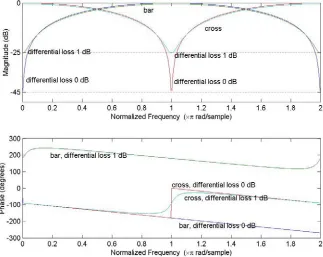
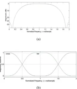
Figure 2.6 shows the magnitude and phase responses of the MZI for various differential losses. Note that the magnitude curves are sine shaped and they have very narrow stopbands. The stopband width at the stopband rejection of –25 dB is only about 4% of the FSR or 8% of the channel spacing. The phase response calculated starts from

90

(29)

Figure 2.6. Magnitude and phase responses of a single-stage Mach-Zehnder Interferometer with differential loss of 0 and 1 dB

2.2.3 Group Delay and Dispersion of the Mach-Zehnder Interferometer

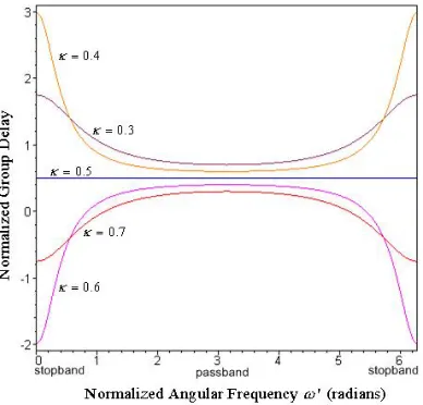
As has been explained in Section 2.1.4, the group delay is derived from the negative derivative of the phase response with respect to the angular frequency. Figure 2.7 shows the normalized group delay of the bar transmission for various power coupling ratios. Each curve shows the values of the normalized group delay versus normalized angular frequency for different power coupling ratios.

(30)

Figure 2.7. Normalized group delay of the bar transmission of Mach-Zehnder Interferometer for various coupling ratios

Figure 2.8. Normalized dispersion of the bar transmission of Mach-Zehnder Interferometer for various coupling ratios

2.3 Lattice Filters of Mach-Zehnder Interferometer

(31)

coupler. Figure 2.9 shows an example of a two-stage lattice filter. It is a 2×2 port device with two input ports and two output ports. It consists of three directional couplers and two delay lines.

In general, an N stage filter has N+1 directional couplers and N delay lines. An N -th order filter can be made wi-th -this multistage configuration. Using -the z-transformation, the filter response can be represented by the polynomial form in z. A synthesis algorithm that can calculate the optical filter parameters from a desired filter response has been presented successfully in literatures [6], [2]. This algorithm uses recursion equations to map the filter coefficients designed with digital filter tools to the power coupling ratios of each directional coupler and the phase of each delay line. Note that although a polynomial filter of a very high order, e.g. order of one hundred, can be realized in digital filters, it is still not possible to realize an optical filter device with a larger number of delay lines due to the chip space restriction and optical losses [1]. Moreover it adds complexity since every additional delay section needs an independent tuning element.

(32)

3 Passband Flattened Filters Design

This chapter describes the mathematical design of the passband flattened interleaver including linear phase filters using Mach-Zehnder interferometer based lattice filters.

3.1 Filter

Requirements

Bandpass optical filters can be used in the binary tree add-drop multiplexer. The filters have to fulfill some requirements. Since the filters are to be used as slicers or interleavers, some specific requirements need to be fulfilled. Below are the desired properties of the slicers:

1. They must have broad passband and stopband so that the available bandwidth can be used as efficiently as possible

2. The passband width must be equal to the stopband width since the wavelength channels are sent to the cross and bar port

3. They must have linear phase response functions in the passband region and hence zero dispersion

4. They have minimal loss at the passband

5. The cross and bar ports fulfill the power conservation rule since the MZI is a passive device

(33)

3.2 Filter Design

Synthesis

In this work, four types of filters are designed. First, a third order passband flattened filter with non-linear phase response is designed followed by a fourth order linear phase passband flattened filter. A fifth order filter with broader stopband width but still having non-linear phase response is built then followed by a seventh order passband flattened filter with linear phase response.

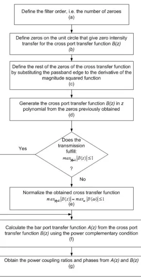
Figure 3.1 summarizes the filters design synthesis process. There are four general steps in the process as described below.

3.2.1 Definition of the Filter Order

In this first step, Figure 3.1(a), the number of zeros, which is equal to the order of the filter, is defined. The number of zeros that can be chosen is three, four, five, or seven depending on the filter order. The number of zeros is related with the desired filter response. The desired filter response can be approximated by placing the zeros on the complex z-plane.

3.2.2 Generation of the Cross Port Transfer Function

This step is as depicted by Figure 3.1(b)-(e). To generate the cross transfer function, the positions of the zeros on the unit circle are described first. These zeros give zero intensity transfer at their normalized frequencies and thus define the stopband width. There are side-lobes in between each zero. Increasing the distance between each zero means that the stopband is broadened, but the side-lobe level also rises. Hence it gives limitation on the stopband width. The zeros are chosen such that the maximum side lobe level is -25 dB.

The rest of the zeros for each filter are defined using the condition that the passband width is equal to the stopband width. Referring to Eq. (2.15), the magnitude squared of a cross transfer function, B(z), with real coefficients is

'

2 ₁

( ) ( ) ( − )

=

= _{z e}j

(34)

(35)

while the transfer function can be written in terms of its roots as

1 1

( ) (1 − )

=

= Γ ∏M −

m m

B z z z (2.56)

Substituting the unity zeros to Eq. (3.2) and applying Eq. (3.1), the magnitude squared function can be represented in terms of the unknown zeros and gain Г. Note that linear phase filters have at least a pair of zeros that is reciprocally mirrored about the unit circle. The maxima of the magnitude squared curve are at the passband edges.

Taking the derivative of Eq. (3.1) with respect to the normalized angular frequency 'ω as zero at the passband edge point, the constant Г could be eliminated and the unknown zeros can be determined. From Eq. (3.1) and (3.2),

' ' ' ' ' ' 2 1 1 1 2 ₁ 2 1 1 2 1 1 1

( ) (1 ) (1 )

d ( ) _d[(1 ₎₍₁ ₎ _]

d( ') d( ')

d[(1 )(1 ) ]

0

d( ')

d[(1 )(1 ) ]

0 d( ') − = = ₌ = − = = = − = = − = = = Γ ∏ − ⋅Γ ∏ − − − = Γ ∏ − − = Γ ∏ − − = ∏ j j j j j j M M

m m m m _{z e}

z e

m m

M

z e z e

m

m m

M z e

m

m m

M z e

m

B z z z z z

B z _{z z} _{z z}

z z z z

ω ω ω ω ω ω ω ω ω ω (2.57)

The derivations of calculations in more details will be explained in next sections for each filter type.

(36)

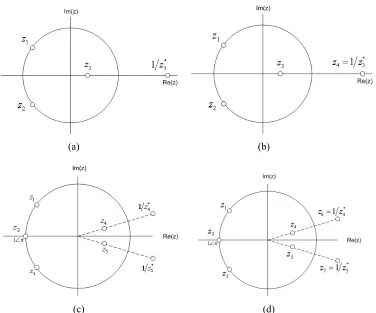
position of the third zero,z₃, can be replaced by its reciprocal mirror * 3

1/z since both zeros give same magnitude response. The same condition applies to the fifth order filter whose unknown fourth and fifth zeros inside the unit circle can be replaced by their mirrors outside the unit circle.

After obtaining all the zeros, the cross transfer function B(z) is calculated using Eq. (3.2) with the gain Г is first considered as equal to one. Then the frequency response of the cross transfer function is calculated. Since the transmission of a passive device such as this Mach-Zehnder interferometer cannot exceed one, the transfer function should be normalized such that the maximum transmission cannot be greater than one. Below is the normalization process performed,

1 ( ) ( ) 1

z

max ₌ B z =max B_ω ω ≤ (2.58)

(a) (b)

(c) (d)

(37)

3.2.3 Calculation of the Bar Port Transfer Function

Once the cross transfer function has been obtained, the bar transfer function can be calculated using the power complementary condition. In this step, Figure 3.1(f), the bar transfer function A(z) is calculated by substituting the normalized cross transfer function

B(z) to the power conservation rule. Recall from Eq. (2.14), the squared magnitude of the bar transfer function can be expressed as

2 _*

( ) ( ) ( )

Aω = Aω A ω (2.59)

2 * *

( ) ( ) (1 )

A z =A z A z (2.60)

From the power conservation rule, the sum of the power of the bar transfer and the cross transfer should be equal to one. Eq. (3.6) can be written as

2 * * * *

0 0 1 * *

1

( ) ( ) (1 ) ( )( )

1 ( ) (1 )

N

k k

k

A z A z A z a a z

z

B z B z

α α

=

= = − −

= −

∏

_(2.61)

where a₀ is the 0-th complex coefficient or the gain of A(z). If the transfer functions have real coefficients then Eq. (3.7) can be written as

2 1 *

0 0 1 1

1

( ) ( ) ( ) ( )( )

1 ( ) ( )

N

k k

k

A z A z A z a a z

z B z B z

α α − = − = = − − = −

∏

_(2.62)

2N zeros of ₁₋_{B z B z}_{( ) (} −1₎_{appears as pairs of}_{( ,1} *₎

k k

α α for k=1∼N. To obtain the bar

transfer function A(z), the N zeros of A(z) must be calculated from (3.8).

Using spectral factorization, each zero of A(z) is defined by selecting one from each pair of zero of 1₋_B(_z)_B*(_z−1)_{. There are 2}N_{selections to obtain the zeroes of}_A₍_z_). Thus, 2N different kinds of A(z) can be obtained from one known B(z). They have the same amplitude characteristics but different phase characteristics.

3.2.4 Obtaining the Optical Parameters

(38)

coefficients of the filter transfer function in a z polynomial to the optical parameters is used. The algorithm uses recursion equations to calculate the power coupling ratios of each directional coupler and the phase of each delay line.

3.3 Third

Order Filter

3.3.1 The Cross Transfer of the Third Order Filter

In order to have a broader stopband width and hence also broader passband width, one zero on the unit circle is added to the single-stage MZI which has only one zero in its transfer function. Now the filter has two zeros, namely z1 and z2, that lie on the unit circle

and hence the stopband is broadened. There is a side-lobe between the two zeros. But the passband is still not flat. The third zero z3 should be placed at a distance in between the

first two zeros but at the other side of the origin of the complex z-plane and not on the unit circle to get a passband flattened. The zeros’ positions of the third order filter are as has been depicted by Figure 3.2(a).

The positions of the two zeros on unit circle are chosen first such that the side-lobe level is -30 dB. Suppose z1 and z2 are chosen as (the angles are given in radians)

1 2

0.9509 0.3094 1 2.827 0.9509 0.3094 1 2.827

z j

= − + = ∠

= − − = ∠ − (2.63)

z3 is the unknown zero and since in this case is real, it can be represented as

3 0

z = +x j (2.64)

The stopband determined by the two zeros on the unit circle lies from normalized angular frequency of 0.9π to 1.1π. Note that the angles are given in radians.

From Eq. (3.2), the cross transfer function can be written as follows

1 1 1

1 2 3

( ) (1 )(1 )(1 )

B z = Γ −z z− −z z− −z z− (2.65)

or in expanded version:

1 2 3

1 2 3 3 1 2 1 2 1 2 3

( ) ( ) ( ( ) ) ( )

(39)

The transfer function can also be written in terms of its coefficients as

1 2 3 0 1 2 3

( )

B z = +c c z− +c z− +c z− (2.67)

Now definitions are made for the part of each coefficient as following

0

1 1 2 3 2 3 1 2 1 2 3 1 2 3

1 ( ) ( ( ) ) ( ) = = − + + = + + = − c

c z z z

c z z z z z

c z z z

(2.68)

Note that c_n = Γ ⋅c_n for n=0∼N. Since z1 and z2 are known and recalling Eq. (3.10),

equations in (3.14) are represented in terms of x. Defining back Eq. (3.12) in terms of Eq. (3.14) and applying Eq. (3.1), the magnitude squared of the cross transfer function can be represented as following

'

3 3

2 ₂ ₍ ₎

0 0 3 3

2 ( ) ' 0 0

( ) j

k l k l z e

k l

k l j k l

k l

B z c c z

c c e

ω ω − − = = = − − = = = Γ = Γ

∑∑

(2.69)

where ck and cl are coefficients components as defined by (3.14) of ( )B z and

1

( )

B z−

respectively. The derivative of Eq. (3.15) with respect to the normalized angular frequency is as follows

2

' ₃ ₃ ₍ ₎ _' 2

0 0 3 3

2 ( ) '

0 0

d ( ) _d( ₎

d( ') d( ')

( ( )) − − = = − − = = = Γ = Γ − −

∑∑

j _{k l j}

k l

k l

k l j k l

k l

B e _e

c c

c c k l e

ω _ω

ω

ω ω _(2.70)

Since the stopband edges are at normalized angular frequencies of 0.9π and 1.1π, the passband edges are found at normalized angular frequencies of 0.1π and 1.9π. Taking Eq. (3.16) as zero at one of those points, x can be found and hence z3 can be determined.

Table 3.1 shows the zeros of the cross transfer function of the third order filter. The third

zero can be chosen either as z3 or its mirror 1/z*3since both of them give same magnitude

(40)

z1 1 2.827∠

z2 1∠ −2.827

z3 0.2841 0∠

* 3

1/z 3.5200 0∠

Table 3.1. Zeros of the cross transfer third order filter

z1 1 2.827∠ z1 1 2.827∠

z2 1∠ −2.827 z2 1∠ −2.827

z3 0.2841 0∠ z3 3.5200 0∠

1 2 3

1( ) 0.3577 0.5786 0.1644 0.1016

B z ₌ ₊ z− ₊ z− ₋ z− 1 2 3

2( ) 0.1016 0.1644 0.5786 0.3577

B z ₌ ₋ z− ₋ z− ₋ z−

Table 3.2. Cross transfer functions of the third order filter

The magnitude squared response of the obtained cross transfer function for B1(z)

is shown by Figure 3.3 and the phase response is shown by Figure 3.4. The stopband width at –25 dB is 15.2% of the FSR or 30.4% of the channel spacing. The side-lobe level is –26.92 dB. The ripple level in the passband is very small, ₋_{8.69 10}_⋅ −3_{dB, thus the}

(41)

(a)

(b)

Figure 3.3. Magnitude squared response of the cross port transfer function of the third order filter (a) in decibel scale and (b) in linear scale

(42)

(a) (b)

Figure 3.5. Normalized (a) group delay and (b) dispersion of the cross port transfer function of the third order filter

3.3.2 The Bar Transfer of the Third Order Filter

From Figure 3.3(b), the cross transfer function magnitude squared curve is symmetric within one period. The zeros of the bar transfer can be found referring to Section 3.2.3. using Eq. (3.8) which are actually can be found also by rotating the zero diagram of the cross transfer by π radians since the cross transfer is symmetric. The zero diagram of the bar transfer of the third order filter is depicted by Figure 3.6. Table 3.3 gives the possible two bar transfer functions for two different zero configurations.

(43)

z1 1 0.314∠ z1 1 0.314∠

z2 1∠ −0.314 z2 1∠ −0.314

z3 0.2841∠π z3 3.5200∠π

1 2 3

1( )z 0.3577 0.5786z 0.1644z 0.1016z

A ₌ ₋ − ₊ − ₊ − 1 2 3

2( )z 0.1016 0.1644z 0.5786z 0.3577z

A ₌ ₊ − ₋ − ₊ −

Table 3.3. Bar transfer functions and their zeros of the third order filter

Figure 3.7(a) shows the magnitude response of the bar transfer in decibel scale and Figure 3.7(b) shows the magnitude squared response of both cross, B1(z), and bar

transfer A1(z) for comparison. Figure 3.8 shows the phase response of the bar transfer.

The phase response also shows a non-linear function. The curves satisfy the power conservation. The normalized group delay and dispersion are shown by Figure 3.9. Note that the responses are the shifted version of those of the cross transfer.

(a)

(b)

(44)

Figure 3.8. Phase response of the bar port transfer function of the third order filter

(a) (b)

Figure 3.9. Normalized (a) group delay and (b) dispersion of the bar port transfer function of the third order filter

3.3.3 The Optical Parameters of the Third Order Filter

From the cross and bar transfer obtained, a three-stage optical filter can represent the third order filter slicer. Appendix D gives the possible configurations of the power coupling constants of each directional coupler and the phases of each delay line calculated using the available simulation tools. For the third order filter, since there are two possible solutions for each bar and cross transfer, there are four possible configurations.

(45)

3.4 Fourth Order Filter

3.4.1 The Cross Transfer of the Fourth Order Filter

As seen previously, the third order filter still has a non-linear phase response and non-zero dispersion in the passband. As explained in the previous chapter, a linear phase filter has at least a pair of zeros that are mirrored about the unit circle. The zeros positions of the fourth order filter are as has been depicted by Figure 3.2(b). The filter will be built with a similar algorithm as for the third order filter.

Suppose now the zeros on the unit circle are still as same as the third order filter:

1 2

0.9509 0.3094 1 2.827 0.9509 0.3094 1 2.827

z j

= − + = ∠

= − − = ∠ − (2.71)

Now the rest two unknown zeros are defined as

3 4

0 1

0

z x j

z j

x

= +

= + (2.72)

The stopband also lies from normalized angular frequency of 0.9π to 1.1π where the transfers are zero at both of those points. The fourth order cross transfer function can be written in terms of its roots as

1 2

1 2 3 4 3 4 4 1 2 3 1 2 1 2

3 4

1 2 3 4 3 4 1 2 1 2 3 4

( ) ( ) [ ( ) ( ) ]

[( ) ( ) ] ( )

B z z z z z z z z z z z z z z z z z

z z z z z z z z z z z z z z

− −

= Γ − Γ + + + + Γ + + + + +

−Γ + + + + Γ (2.73)

or in terms of its coefficients as

1 2 3 4 0 1 2 3 4

( )

B z _{= +}c c z− ₊c z− ₊c z− ₊c z− _(2.74)

The following definitions are made:

0

1 1 2 3 4

2 3 4 4 1 2 3 1 2 1 2 3 1 2 3 4 3 4 1 2 4 1 2 3 4

1

( )

( ) ( )

[( ) ( ) ]

c

c z z z z

c z z z z z z z z z z

c z z z z z z z z

c z z z z

= = − + + + = + + + + + = − + + + = (2.75)

(46)

emerges

'

4 4

2 ₂ ₍ ₎

0 0 4 4

2 ( ) ' 0 0

( ) j

k l k l z e

k l

k l j k l

k l

B z c c z

c c e

ω ω − − = = = − − = = = Γ = Γ

∑∑

(2.76)

The derivative of the magnitude squared with respect to the normalized angular frequency is as follows

2

' ₄ ₄ ₍ ₎ _' 2

0 0 4 4

2 ( ) '

0 0

d ( ) _d( ₎

d( ') d( ')

( ( )) − − = = − − = = = Γ = Γ − −

∑∑

j _{k l j}

k l

k l

k l j k l

k l

B e _e

c c

c c k l e

ω _ω

ω

ω ω _(2.77)

As done with the third order filter, z3 and z4 can be found by substituting the

normalized angular frequency that defines the passband edge to Eq. (3.23) and taking the value of (3.23) as zero. The passband edges are found at normalized angular frequencies of 0.1π and 1.9π. Zeros found for the fourth order filter are:

1 2 3 4 1 2.827 1 2.827 0.1810 0 5.5250 0 z z z z = ∠ = ∠ − = ∠ = ∠ (2.78)

The cross transfer function obtained with zeros in (3.24) is

1 2 3 4

( ) 0.0691 0.2629 0.6118 0.2629 0.0691

B z ₌ ₋ z− ₋ z− ₋ z− ₊ z− _(2.79)

Note that the transfer function is a mirror-image polynomial as referred to Chapter 2 or Appendix A.

The magnitude squared response of the obtained cross transfer function B(z) is shown by Figure 3.10 and the phase response is shown by Figure 3.11. The stopband width at –25 dB is 14.6% of the FSR or 29.2% of the channel spacing. The side-lobe level is –25.63 dB. Seems that addition of a zero at the passband increases the side-lobe level and hence decreases the –25 dB stopband width compared to the third order filter. The ripple level in the passband is₋_{6.08 10}_⋅ −3_{dB. The phase response is linear at the passband.}

(47)

(a) (b)

Figure 3.10. Magnitude squared response of the cross port transfer function of the fourth order filter in (a) decibel scale and (b) linear scale

Figure 3.11. Phase response of the cross port transfer function of the fourth order filter

3.4.2 The Bar Transfer of the Fourth Order Filter

(48)

Given zeros:

1 2 3 4

1 3.14

1 0.314

3.1618 7.1500 0

z z z z

π

= ∠ = ∠ −

= ∠

(2.80)

the bar transfer obtained is

1 2 3 4

( ) 0.0145 0.0856 0.2037 0.5666 0.3284

A z = − z− − z− + z− − z− (2.81)

Figure 3.12. Zero diagram of the bar transfer fourth order filter

Figure 3.13(a) shows the magnitude response of the bar transfer in decibel scale while Figure 3.13(b) shows the magnitude squared response of both cross transfer B(z) and bar transfer A(z) for comparison. Figure 3.14 shows the phase response of the bar transfer. Since the zeros do not comprise of zeros that are mirrored each other about the unit circle anymore, it has a non-linear phase response. Hence the group delay is not constant and the dispersion is not zero.

(49)

For the bar transfer function as defined by Eq. (3.27), the reverse polynomial is

1 2 3 4

( ) 0.3284 0.5666 0.2037 0.0856 0.0145

R

A z _{= −} ₊ z− ₋ z− ₋ z− ₊ z− _(2.82)

(a)

(b)

Figure 3.13. Magnitude response of the bar transfer function fourth order filter in decibel scale (a) and magnitude squared response of the bar and cross transfer of the fourth order filter (b)

(50)

and its reverse function are shown by Figure 3.15. As can be seen from the graphs, although the dispersion of each function is not equal to zero, but they are compensates each other. Hence they may produce a zero dispersion at the bar output port.

(a) (b)

Figure 3.15. Normalized (a) group delay and (b) dispersion of the bar port transfer function of the fourth order filter and its reverse polynomial

3.4.3 The Optical Parameters of the Fourth Order Filter

The optical filter parameters are obtained from the generated bar transfer and cross transfer A(z) and B(z). Note that _{B z}R( )₌_{B z}( )_{. In Appendix D, Table D.2 gives the} power coupling constant of each directional coupler and the phase of each delay line. It gives two configurations, one is for the splitting part and the other is for the combining part with the reverse bar transfer function. The filter coefficients can be mapped to a four-stage optical filter with five couplers and four delay lines.

3.5 Fifth

Order Filter

3.5.1 The Cross Transfer of the Fifth Order Filter

The fifth order filter zero diagram is as has been shown by Figure 3.2(c). In order to have a broader stopband width compared to the third and fourth order filters, three zeros are put on the unit circle. They are, namely z1, z2, and z3. The fourth and fifth

zeroes, namely z4 and z5, are not on the unit circle and will be placed at the opposite side

(51)

At first, the positions of the three zeroes on the unit circle are chosen, then the fourth and fifth zeroes will be found through calculation. The calculation algorithm is similar with the previous filter designs. If the three zeroes on the unit circle are chosen first such that the side lobe level in between is –30 dB, the result with the five zeroes is shown a rising of the side lobe level of 12 dB. Hence the positions of the three zeroes are chosen first such that the maximum side lobe level is –40 dB in order to anticipate the final response with five zeroes will have side lobe level not greater than –25 dB. Moreover the addition of two more zeroes to design the next seventh order filter should be anticipated to have a side lobe level also not greater than –25 dB.

The zeros on unit circle are chosen as

1 2 3

0.8265 0.5629 1 2.544

1 0 1

0.8265 0.5629 1 2.544

z j z j z j π = − + = ∠ = − + = ∠ = − − = ∠ − (2.83)

The remaining two unknown zeros are defined as

4 5

z x jy

= +

= − (2.84)

with x and y are the real and imaginary parts of z4 and z5.

The stopband determined by the three zeros on the unit circle lies from the normalized angular frequency of 0.81π to 1.19π. The fifth order cross transfer function can be written in terms of its roots as

1

-1

2 3 4 5 4 5 3 5 3 4 2 5 2 4 2 3 1 5 1 4 -2

1 3 1 2 3 4 5 2 4 5 2 3 5 2 3 4 1 4 5 1 3 5 1 3 4 1 2 5 -3

1 2 4 1 2 3 2 3 4 5 1 3 4 5 1 2 4 5 1 2 3 5 1

( ) ( ) (

) (

B z z z z z z z z z z z z z z z z z z z z z z z

z z z z z z z z z z z z z z z z z z z z z z z z z z z z z

z z z z z z z z z z z z z z z z z z z z z z z z

= Γ − Γ + + + + + Γ + + + + + + +

+ + − Γ + + + + + + +

+ + + Γ + + + + -4

2 3 4 5

1 2 3 4 5

)

( )

z z z z z z z z z z−

− Γ

(52)

The following definitions are made,

1

0

1 2 3 4 5

2 4 5 3 5 3 4 2 5 2 4 2 3 1 5 1 4 1 3 1 2

3 3 4 5 2 4 5 2 3 5 2 3 4 1 4 5 1 3 5 1 3 4 1 2 5 1 2 4 1 2 3 4 2 3 4 5 1 3 4 5 1 2 4 5 1 2 3 5 1

1 ( ) ( ) ( ) ( c

c z z z z z

c z z z z z z z z z z z z z z z z z z z z

c z z z z z z z z z z z z z z z z z z z z z z z z z z z z z z

c z z z z z z z z z z z z z z z z z

=

= − + + + +

= + + + + + + + + +

= − + + + + + + + + +

= + + + + _{2 3 4}

5 1 2 3 4 5

)

z z z c =z z z z z

(2.86)

Substituting (3.29) and (3.30) to Eq. (3.32) and defining Eq. (3.31) in terms of (3.32), then taking the magnitude squared of the cross transfer function, the following equation emerges

'

5 5

2 ₂ ₍ ₎

0 0 5 5

2 ( ) ' 0 0

( ) j

k l k l z e

k l

k l j k l

k l

B z c c z

c c e

ω ω − − = = = − − = = = Γ = Γ

∑∑

(2.87)

The derivative of the magnitude squared with respect to the normalized angular frequency is as follows

2

' ₍ ₎ _'

2 0 0 5 5

2 ( ) '

0 0

d ( ) _d( ₎

d( ') d( ')

( ( )) − − = = − − = = = Γ = Γ − −

∑∑

j _{k l j}

k l

k l

k l j k l

k l

B e _e

c c

c c k l e

ω _ω

ω

ω ω _(2.88)

For the fifth order filter, z4 and z5 can be found by taking the value of (3.33) as

zero at two points, one is at the passband edge point and the other is at half-width of the passband which is related with the side lobe position in the stopband. Table 3.4 shows the zeros of the cross transfer function of the fifth order filter. The fourth zero can be chosen between z4 and its mirror 1 z*4 since both of them give identical magnitude response

although they have different phase responses, and so can the fifth zero be chosen between z5 and its mirror 1 z*5. It results into four possible cross transfer functions that can be

(53)

z1 1 2.544∠

z2 1∠π

z3 1∠ −2.544

z4 0.3724 0.511∠

* 4

1 z 2.6859 0.511∠

z5 0.3724∠ −0.511

* 5

1 z 2.6859∠ −0.511

Table 3.4. Zeros of the cross transfer fifth order filter

Taking zeros of: