Taxonomy Learning Using Word Sense Induction

Taxonomy Learning Using Word Sense Induction

Ioannis P. Klapaftis

Department of Computer Science The University of York

York, UK, YO10 5DD [email protected]

Suresh Manandhar

Department of Computer Science The University of York

York, UK, YO10 5DD [email protected]

Abstract

Taxonomies are an important resource for a variety of Natural Language Processing (NLP) applications. Despite this, the current state-of-the-art methods in taxonomy learning have disregarded word polysemy, in effect, devel-oping taxonomies that conflate word senses. In this paper, we present an unsupervised method that builds a taxonomy of senses learned automatically from an unlabelled cor-pus. Our evaluation on two WordNet-derived taxonomies shows that the learned taxonomies capture a higher number of correct taxonomic relations compared to those produced by tradi-tional distributradi-tional similarity approaches that merge senses by grouping the features of each word into a single vector.

1 Introduction

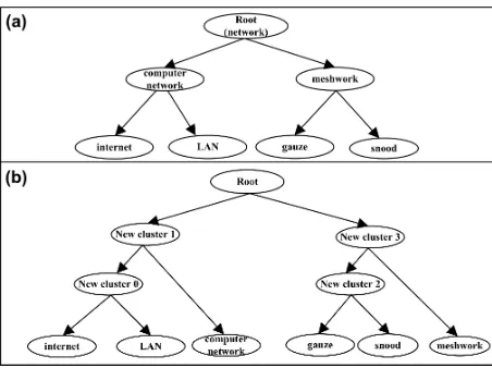
A concept or a sense,s, can be defined as the mean-ing of a word or a multiword expression. A con-ceptscan be linguistically realised by more than one word while at the same time a wordwcan be the lin-guistic realisation of more than one concept. Given a set of conceptsS, taxonomy learning is the task of hierarchically classifying the elements inSin an au-tomaticmanner. For example, consider a set of con-cepts linguistically realised by the words/multiword expressionsLAN, computer network, internet, mesh-work, gauze, snood. Taxonomy learning methods produce taxonomies, such as the ones shown in Fig-ures 1 (a) and 1 (b).

By observing Figure 1 (a), we can express IS-Astatements, such asInternetIS-AComputer Net-worketc. However, the same does not apply to the

Figure 1: A labelled and an unlabelled concept taxonomy

taxonomy in Figure 1 (b), since this taxonomy is not fully labelled. Despite this, its hierarchical organ-isation clearly shows that the concepts are divided into groups, which are further subdivided into sub-groups and so forth, until we reach a level where each concept belongs to its own group. Unlabelled taxonomies are typically produced by agglomera-tive hierarchical clustering algorithms (King, 1967; Sneath and Sokal, 1973).

The knowledge encoded in taxonomies can be utilised in a range of NLP applications. For in-stance, taxonomies can be used in information trieval to expand a user query with semantically re-lated words or to enhance document representation by abstracting from plain words and adding concep-tual information (Cimiano, 2006). WordNet’s (Fell-baum, 1998) taxonomic relations have also been used in Word Sense Disambiguation (WSD) (Nav-igli and Velardi, 2004b). In named entity recog-nition, methods relying on gazetteers could make

use of automatically acquired taxonomies (Cimiano, 2006), while question answering systems have also benefited (Moldovan and Novischi, 2002).

Despite the wide uses of taxonomies, the majority of methods disregard or do not deal effectively with word polysemy, in effect, developing taxonomies that conflate the senses of words (see Section 2). In this work, we show that Word Sense Induction (WSI) can be effectively employed to address this limitation of existing methods.

We present a novel method that employs WSI to generate the different senses of a set of target words from an unlabelled corpus and then produces a tax-onomy of senses using Hierarchical Agglomerative Clustering (HAC) (King, 1967; Sneath and Sokal, 1973). We evaluate our method on two WordNet-derived sub-taxonomies and show that our method leads to the development of concept hierarchies that capture a higher number of correct taxonomic rela-tions in comparison to those generated by current distributional similarity approaches.

2 Related work

Initial research on taxonomy learning focused on identifying in a given text lexico-syntactic patterns that suggest hyponymy relations (Hearst, 1992). For instance, the pattern N P0 such as N P1,. . . ,N Pn

suggests that N P0 is a hypernym ofN Pi. For

ex-ample, given the phraseFruits, such as oranges, ap-ples,..., the above pattern would suggest that fruit is a hypernym oforangeandapple. These pattern-based approaches operate at the word level by learn-ing lexical relations between words rather than be-tween senses of words.

In the same spirit, other work attempted to exploit the regularities of dictionary entries to identify hy-ponymy relations (Amsler, 1981). For example in WordNet, WAN is defined as a computer network that spans . . .. Hence, one can easily induce that WANis a hyponym ofcomputer networkby assum-ing that the first noun phrase in the definition is a hy-pernym of the target word. These approaches learn lexical relations at the sense level since dictionaries separate the senses of a word. However this would be true if and only if the glosses of the dictionaries were sense-annotated, which is not the case for the majority of electronic dictionaries (Cimiano, 2006).

Another limitation is that taxonomies are built ac-cording to the sense distinctions present in dictio-naries and not according to the actual use of words in the corpus.

The majority of taxonomy learning approaches are based on the distributional hypothesis (Harris, 1968). Typically, distributional similarity methods (Cimiano et al., 2004; Cimiano et al., 2005; Faure and N´edellec, 1998; Reinberger and Spyns, 2004; Caraballo, 1999) utilise syntactic dependencies such as subject/verb, object/verb relations, conjunctive and appositive constructions and others. These de-pendencies are used to extract the features that serve as the dimensions of the vector space. Each target noun is then represented as a vector of extracted fea-tures where the frequency of co-occurrence of the target noun with each feature is used to calculate the weight of that feature. The constructed vectors are the input to hierarchical clustering orformal concept analysis(Ganter and Wille, 1999) to produce a tax-onomy. These approaches assume that a target noun is monosemous creating one vector of features for each target noun. This limitation can lead to a num-ber of problems.

Firstly, the constructed taxonomies might be bi-ased towards the inclusion of taxonomic relation-ships between the most frequent senses of tar-get nouns, ignoring interesting taxonomic relations where less frequent senses are present. For exam-ple, consider the wordhouse. Current distributional similarity methods would possibly capture the hy-ponyms of its Most Frequent Sense (MFS1), how-ever ignoring the hyponyms of less frequent senses ofhouse, e.g. casino,theater, etc. Given that word senses typically follow a Zipf distribution, these methods construct vectors dominated by the MFS of words. This bias significantly degrades the useful-ness of learned taxonomies.

Secondly, given that distributional similarity ap-proaches rely on the computation of pairwise simi-larities between target words, merging their senses to a single vector might lead to unreliable similarity estimates. For example, merging the features of the different senses ofhousecould provide a lower sim-ilarity with its monosemous hyponymbeach house, since only the first sense ofhouseis related tobeach

1

house. This problem might lead both to inclusion of incorrect or loss of correct taxonomic relations. In our work, we aim to overcome these drawbacks by identifying the different senses with which target words appear in text and then building a hierarchy of the identified senses.

Soft clustering approaches (Reinberger and Spyns, 2004; Reinberger et al., 2003) have also been applied to taxonomy learning to deal with polysemy. These methods associate each verb with a vector of features, where each feature is a noun appearing as a subject or object of that verb. That way a noun can appear in different vectors, hence in different clus-ters during hierarchical clustering as a result of its polysemy. However, the underlying assumption is that a verb is monosemous with respect to its associ-ated vector of nouns. This assumption is not always valid and can cause the problems mentioned above.

Other work in taxonomy learning exploits the head/modifier relationships to create taxonomic re-lations (Buitelaar et al., 2004; Hwang, 1999; S´anchez and Moreno, 2005). These relations are used to create: (1) a class (concept) for each head, and (2) subclasses by adding nominal or adjectival modifiers. For example,credit cardIS-Acard. The corresponding hyponymy relations are learned at the lexical level disregarding word polysemy. Some of these approaches identified the problem of polysemy and applied sense disambiguation with respect to WordNet in order to capture the different senses of a target term (Navigli and Velardi, 2004b; Navigli and Velardi, 2004a). Specifically, the taxonomy built by exploiting head/modifiers relations was modified ac-cording to WordNet’s hyponymy relations between senses of disambiguated terms. One important de-ficiency of using sense disambiguation is that dic-tionaries miss many domain-specific senses. Addi-tionally, the fixed-list of senses paradigm prohibits learning word senses according to their use in con-text. The use of sense induction we propose in this paper aims to overcome these limitations.

3 Method

Given a set of wordsW, a WSI method is applied to eachwi ∈ W (Section 3.1). The outcome of the

first stage is a set of senses,S, where eachsw_i ∈ S

denotes the i-th sense of word w ∈ W. This set

Figure 2: WSI fornetwork&LAN

of senses is the input to hierarchical clustering that produces a hierarchy of senses (Section 3.2).

3.1 Word sense induction

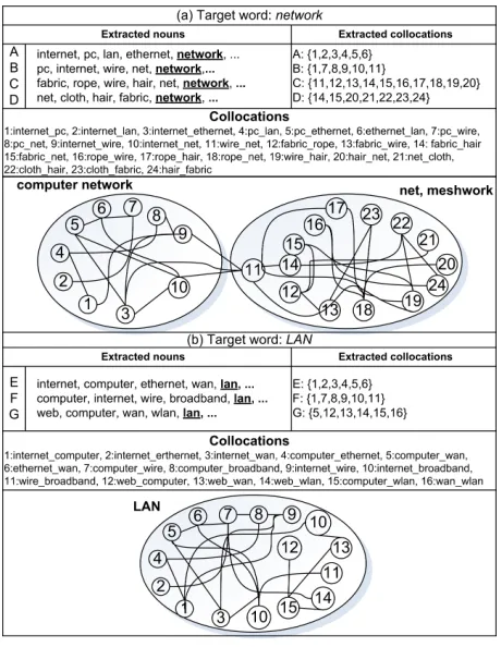
WSI is the task of identifying the senses of a tar-get word in a given text. Recent WSI methods were evaluated under the framework of SemEval-2007 WSI task (SWSI) (Agirre and Soroa, SemEval-2007). The evaluation framework defines two types of as-sessment, i.e. evaluation in: (1) a clustering and (2) a WSD setting. Based on this evaluation, we se-lected the method of Klapaftis & Manandhar (2008) (henceforth referred to as KM) that achieves high F-score in both evaluation schemes as compared to the systems participating in SWSI. We briefly describe KM mentioning its parameters used in our evalua-tion (Secevalua-tion 4). Figures 2 (a) and 2 (b) describe the different steps for inducing the senses of the target wordsnetworkandLAN.

related to w. Initially, the target word is removed from bc, part-of-speech tagging is applied to each paragraph, only nouns are kept and lemmatised. In the next step, the distribution of each noun is com-pared to the distribution of the same noun in a ref-erence corpus2 using the log-likelihood ratio (G2) (Dunning, 1993). Nouns with a G2 below a pre-specified threshold (parameterp1) are removed from

each paragraph. Figure 2 (a) shows the remaining nouns for each paragraph ofbc.

Graph creation & clustering: In the setting of KM, a collocation is a juxtaposition of two nouns within the same paragraph. Thus, each noun is com-bined with any other noun yielding a total of N₂

collocations for a paragraph with N nouns. Each collocation,cij, is assigned a weight that measures

the relative frequency of two nouns co-occurring. This weight is the average of the conditional prob-abilities p(ni|nj) and p(nj|ni), where p(ni|nj) =

f(cij)

f(nj),f(cij)is the number of paragraphs nounsni,

nj co-occur andf(nj)is the number of paragraphs

in whichnj appears. Collocations are filtered with

respect to their frequency (parameterp2) and weight

(parameter p3). Each retained collocation is

rep-resented as a vertex. Edges between vertices are present, if two collocations co-occur in one or more paragraphs. Figure 2 (a) shows that this process has generated 24 collocations for the target word net-work. On the top right of the figure we also observe the collocations associated with each paragraph.

In the next step, a smoothing technique is applied to discover new edges between vertices. The weight applied to each edge connecting vertices vi and vj

(collocationscab,cde) is the maximum of their

con-ditional probabilities (max(p(cab|cde), p(cde|cab))).

Finally, the graph is clustered using Chinese whis-pers (Biemann, 2006). The final output is a set of senses, each one represented by a set of contextually related collocations. In Figure 2, we generated two senses fornetworkand one sense forLAN.

3.2 Hierarchical clustering of senses

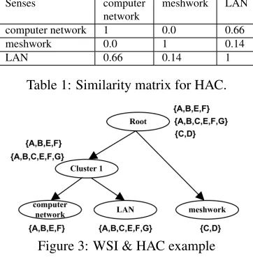
Given the set of sensesS, our task at this point is to hierarchically classify the senses using HAC. Con-sider for example the wordsnetworkandLAN, and

2_{The British National Corpus, 2001, Distributed by Oxford} University Computing Services.

Senses computer meshwork LAN network

computer network 1 0.0 0.66 meshwork 0.0 1 0.14 LAN 0.66 0.14 1

Table 1: Similarity matrix for HAC.

Figure 3: WSI & HAC example

let us assume that the WSI process has generated the senses in Figures 2 (a) and 2 (b). HAC oper-ates by treating each sense as a singleton cluster and then successively merging the most similar clusters according to a pre-defined similarity function. This process iterates until all clusters have been merged into a single cluster taken to be theroot.

To calculate the pairwise similarities between senses we exploit the attributes that represent each sense, i.e. their collocations. LetBC be the cor-pus resulting from the union of the base corpora of all words inW. In our example,BCwould consist of the paragraphs, in which the wordsnetworkand LANappear, i.e. A,B,...,G. An induced sense tags a paragraph, if one or more of its collocations ap-pear in that paragraph. Thus, each induced sense is associated with a set of paragraph labels that denote the paragraphs tagged by that sense. Figure 3 shows the paragraph labels tagged by each sense of our ex-ample. Finally, given two senses sa_i, sb_i and their corresponding sets of tagged paragraphsf_iaandf_ib, we use the Jaccard coefficient to calculate their sim-ilarity, i.e. JC(sa

i, sbi) =

|fai∩f b i|

|fa i∪f

b i|

, where sk

j denotes

the j-th sense of wordk. The resulting similarity matrix of our example is shown in Table 1. Given that matrix, HAC would first group computer net-work and LAN as they have the highest similarity (Figure 3). In the final iteration, the remaining two clusters (Cluster 1&meshwork) would be grouped to theroot.

the taxonomy clusters contain more than one sets of tagged paragraphs (Figure 3 -Cluster 1), hence the choice of the similarity function is crucial. We ex-periment with three techniques, i.e. single-linkage, complete-linkageandaverage-linkage. The first one defines the similarity between two clusters as the maximum similarity among all the pairs of their cor-responding feature sets. The second considers the minimum similarity among all the pairs, while the third calculates the average similarity of all the pairs.

4 Evaluation

We evaluate our method with respect to two WordNet-derived sub-taxonomies (Section 4.3). For that reason, it is necessary to map the induced senses to WordNet before applying HAC. Note that the mapping process might map more than one induced senses to the same WordNet sense. In that case, these induced senses are merged to a single one along with their corresponding collocations.

4.1 Mapping WSI clusters to WordNet senses

The process of mapping the induced senses to Word-Net is straightforward. Letw ∈ W be a word with

nsenses in WordNet. A WordNet senseiofwis de-noted bywsw_i ,i= [1, n]. Let us also assume that the WSI method has produced m senses for w, where each sensejis denoted assw_j,j = [1, m]. Each in-duced sense sw_j is associated with a set of features

f_jwas in the previous section. These features are the paragraphs (paragraph labels) ofBC tagged bysw_j. In the next step, each WordNet sensewsw_i is associ-ated with its WordNet signaturegw_i that contains the following semantic features: hypernyms/hyponyms, meronyms/holonyms and synonyms of wsw

i . For

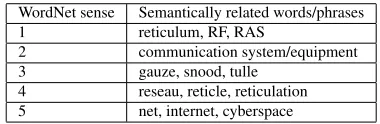
example, the signature of the fifth WordNet sense ofnetworkwould contain internet, cyberspace and other semantically related words. Table 2 shows par-tial signatures for each sense ofnetwork.

The signature g_iw is used to formalise the Word-Net sensewsw_i as a set of featuresqw_i . These fea-tures are the paragraphs (paragraph labels) of BC

that contain one or more of the aforementioned se-mantically related to wsw_i words that exist in g_iw. Given an induced sensesw_j, a similarity score is cal-culated betweensw_j and each WordNet sense of w. The maximum score determines the WordNet sense

WordNet sense Semantically related words/phrases 1 reticulum, RF, RAS

2 communication system/equipment 3 gauze, snood, tulle

4 reseau, reticle, reticulation 5 net, internet, cyberspace

Table 2: Semantically related words/phrases tonetwork

label that will be assigned tosw_j, i.e. label(sw_j) = argmax_iJ C(f_jw, q_iw), whereJ Cis the Jaccard sim-ilarity coefficient. In the example of Figure 2 (a), thecomputer networksense would be mapped to the fifth WordNet sense ofnetwork, since there is a sig-nificant overlap between the paragraphs tagged by the induced and that WordNet sense.

4.2 Evaluation measures

For the purposes of this section we present one gold standard taxonomy (Figure 1 (a)) and a second de-rived from our method (Figure 1 (b)). The compari-son of these taxonomies is based on thesemantic co-topyof a node, which has also been used in (Maed-che and Staab, 2002; Cimiano et al., 2005). In par-ticular, the semantic cotopy of a node is defined as the set of all its super- and subnodes excluding the rootand including that node. For example, the se-mantic cotopy ofcomputer networkin Figure 1 (a) is {computer network, internet, LAN}. There are two issues, which make the evaluation difficult.

The first one is that HAC produces a taxonomy in which all internal nodes are unlabelled, as opposed to the gold standard taxonomy. In Figure 1 (b), we have manually labelled internal nodes with their IDs for clarity. For example, the semantic cotopy of the nodeNew Cluster 1in Figure 1 (b) is{computer net-work, internet, LAN, New Cluster 1, New Cluster 0}. By comparing the cotopies of nodescomputer networkin Figure 1 (a) and New Cluster 1in Fig-ure 1 (b), we observe that the automatic method has successfully grouped all of the hypernyms and hy-ponyms ofcomputer networkunderNew Cluster 1. However, the corresponding cotopies are not iden-tical, because the cotopy ofNew Cluster 1also in-cludes the labels produced by HAC.

Figure 1 (a) will yield maximum similarity.

The second issue is that the nodes that exist in the gold standard taxonomy are leaf nodes in the auto-matically learned taxonomy. As a result, the seman-tic cotopy of LAN in Figure 1 (b) is {LAN} since all of its supernodes do not exist in WordNet. In contrast, the semantic cotopy of LAN in Figure 1 (a) is {LAN, computer network}. We observe that there is an overlap between the two cotopies derived by the existence of the same concept in both tax-onomies, i.e. LAN. In fact, all of the leaf nodes of a learned taxonomy will have a small overlap with the corresponding concept in the gold standard. For this problem, we observe that in our automatically learned taxonomies it does not make sense to cal-culate the semantic cotopy of leaf nodes. On the contrary, we need to evaluate the internal nodes that group the leaf nodes. Let us assume the following notation:

TA=automatically learned taxonomy

ηi =node in a taxonomy

C(TA) =internal nodes + leaf nodes ofTA

I(TA) =internal nodes ofTA

TG=gold standard taxonomy

C(TG) =internal nodes + leaf nodes ofTG

I(TG) =internal nodes ofTG

hyper(ηi) =supernodes ofηiexcluding the root

hypo(ηi) =subnodes ofηi includingηi

Forηi∈I(TA), the semantic cotopy is defined as:

SC0(ηi) = (hyper(ηi)∪hypo(ηi))∩C(TG)

Forηi∈C(TG), the semantic cotopy is defined as:

SC00(ηi) = (hyper(ηi)∪hypo(ηi))

P(ηi, ηj) =

|SC0(ηi)∩SC00(ηj)|

|SC0_(η

i)|

(1)

R(ηi, ηj) =

|SC0(ηi)∩SC00(ηj)|

|SC00_(η

j)|

(2)

F(ηi, ηj) =

2P(ηi, ηj)R(ηi, ηj)

P(ηi, ηj) +R(ηi, ηj)

(3)

Precision, recall and harmonic mean of nodeηi ∈

I(TA) with respect to node ηj ∈ C(TG) are

de-fined in Equations 1, 2 and 3. The F-score, F S, of nodeηi ∈I(TA)is the maximumF attained at any

ηj ∈ C(TG) (F S(ηi) = argmaxjF(ηi, ηj)).

Fi-nally, the similarity T S of the entire taxonomy to the gold standard taxonomy is the average of the F-scores of each ηi ∈ I(TA) (Equation 4). The

T S(TA, TG) in Figure 1 is 0.9. All nodes of TA

have a perfect match, apart fromNew Cluster 0and New Cluster 2, which are matched againstcomputer network and meshwork respectively, having a per-fect precision but a lower recall since the cotopies ofcomputer networkandmeshworkconsist of three concepts. The automatically learned taxonomy has two redundant clusters that decrease its similarity.

T S(TA, TG) =

1

|I(TA)|

X

ηi∈I(TA)

F S(ηi) (4)

The similarity measure T S(TA, TG) provides the

similarity of the automatically learned taxonomy to the gold standard one, but it is not symmetric. Cal-culating the taxonomic similarity one way might not provide accurate results, in cases whereTAmisses

senses of the gold standard. This is due to the fact that we would only evaluate the internal nodes of TA, partially ignoring the fact that TA might

have missed some parts of the gold standard taxon-omy. For that reason, we also calculateT S(TG, TA)

which provides the similarity of the gold standard taxonomy to the automatically learned one. Fi-nally, taxonomic similarities are combined to pro-duce their harmonic mean (Equation 5).

T xSm(TA, TG) =

2T S(TG, TA)T S(TA, TG)

T S(TG, TA) +T S(TA, TG)

(5)

4.3 Evaluation datasets & setting

The first gold standard taxonomy is derived by ex-tracting from WordNet all the hyponyms of the senses of the wordnetwork. The extracted taxonomy contains 29 senses linguistically realized by 24 word sets (one sense might be expressed with more than one words), sincenetwork has 5 senses andreseau has 2 senses in the gold standard taxonomy. Note that we have disregarded senses only expressed by multiword expressions. The average polysemy of words is around 1.7. The second taxonomy is de-rived by extracting the concepts under the senses of the wordspeaker. Thespeaker taxonomy contains 52 senses linguistically realized by 50 word sets, sincespeakerhas 3 senses included in the taxonomy. The average polysemy of words is around 1.58.

To create our datasets3we use theYahoo! search api4. For each wordwin each of the datasets, we

is-3

Available in http://www.cs.york.ac.uk/aig/projects/indect/taxlearn 4

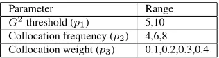
Parameter Range

G2_{threshold (p}

1) 5,10

Collocation frequency (p2) 4,6,8

Collocation weight (p3) 0.1,0.2,0.3,0.4

Table 3: Chosen parameters for the KM WSI method.

sue a query toYahoo!that containswand we down-load a maximum of 1000 pages. In cases where a particular sense is expressed by more than one word, the query was formulated by including all the words and putting the keywordOR between them. For each page we extracted fragments of text (para-graphs) that occur in<p> </p>html tags. We ex-tracted 58956 and 78691 paragraphs for thenetwork andspeakerdataset respectively. The reason we ex-tracted on average less content for the second dataset was thatYahoo! provided a small number of results for rare words such asalliterator,anecdotist, etc.

Table 3 shows the parameter ranges for the WSI method. Our method is evaluated according to these parameters. Our first baseline isRAND, which per-forms a random hierarchical clustering of senses to produce a binary tree. In each iteration two clusters are randomly chosen and form a new cluster, until we end up with one cluster taken to be the root. The performance ofRANDis calculated by executing the random algorithm 10 times and then averaging the results. The second baseline is the taxonomy most frequent sense baseline (TL MFS), in which we do not perform WSI. Instead, given a parameter setting and a wordw, all the collocations ofware grouped into one vector, which will possibly be dominated by collocations related to the MFS ofw. WordNet mapping takes place and finally HAC with average-linkage is applied to create the taxonomy.

4.4 Results & discussion

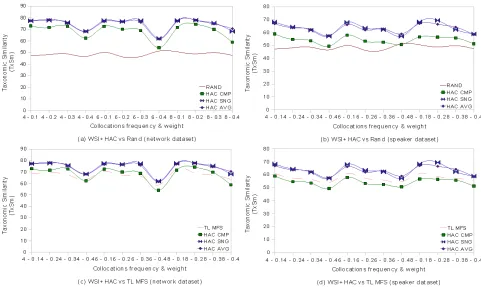
Figures 4 (a) and 4 (b) show the performance of HAC with single-linkage (HAC SNG), average-linkage (HAC AVG) and complete-linkage (HAC CMP) againstRANDforp1 = 5and different

com-binations ofp2andp3. It is clear thatHAC SNGand

HAC AVGoutperformRANDby very large margins under all parameter combinations. In the network dataset, both of them achieve their highest distance fromRAND(27.84%) atp2 = 8andp3= 0.2. In the

speaker dataset, their highest distance fromRAND (20.97% and 19.63% respectively) is achieved at

p2 = 4andp3 = 0.1. HAC CMPperforms worse

than the other HAC versions, yet it clearly outper-formsRANDin all but one parameter combinations (p1 = 5,p2 = 6,p3= 0.4) in thespeaker dataset.

Generally, for collocation weight equal to 0.4 the performance of all HAC versions drops. At this high collocation weight the WSI method produces a larger number of small clusters than in lower thresh-olds. This issue negatively affects both the map-ping process and HAC. For example in thespeaker dataset, forp1 = 5, p2 = 8 andp3 = 0.1 our

onomies contained 86.54% of the gold standard tax-onomy senses. Increasing the collocation weight to 0.2 did not have any effect, but increasing the weight to 0.3 and then 0.4 led to 71.15% and 65.38% sense coverage. Overall, our conclusion is that all HAC versions exploit the WSI method and learn useful information better than chance. The picture is the same forp1 = 10.

Figures 4 (c) and 4 (d) show the performance of HAC versions against the TL MFS baseline in the same parameter setting as above. We observe that bothHAC SNGandHAC AVGperform significantly better thanTL MFSapart fromp3 = 0.4, in which

case allHACversions perform worse. In thenetwork dataset, the largest performance difference forHAC SNGis 10.12% and forHAC AVG9.9% atp2 = 6

andp3 = 0.2. In thespeakerdataset, the largest

per-formance difference for HAC SNG is 10.83% and forHAC AVG7.83% atp2 = 8andp3 = 0.2. HAC

CMPperforms worse thanTL MFSunder most pa-rameter settings in both datasets. The picture is the same forp1 = 10.

Figure 4: Performance analysis of the proposed method forp1= 5and different combinations ofp2andp3.

Despite that, our evaluation also shows that in most cases HAC CMP is unable to exploit the in-duced senses and performs worse than TL MFS, HAC SNG and HAC AVG. This result was not ex-pected, sinceHAC SNGemploys a local criterion to merge two clusters and does not consider the global structure of the clusters, in effect, being biased to-wards elongated clusters. The observation of the gold standard taxonomies shows that they consist both of cohyponym concepts which are expected to be contextually related, but also of cohyponyms which are not expected to appear in similar contexts. For example, someone would expect a high similar-ity betweenWAN,LAN, or betweensnoodandtulle. However, the same does not apply for snood and cheeseclothortulle andgrillwork, because cheese-clothandgrillworkappear in significantly different contexts than snood andtulle. Despite that, all of them are cohyponyms. This issue is more prevalent in thespeakerdataset, where concepts such as loud-speaker,tannoy,woofer are expected to be contex-tually related, while cohyponyms such aswhisperer, lecturerandinterviewerare not. This means that the gold standard taxonomies include elongated clusters and explains the superior performance ofHAC SNG.

This issue is not affectingHAC AVG, but it has a sig-nificant effect onHAC CMP. Generally, HAC CMP employs a non-local criterion by considering the di-ameter of a candidate cluster. This results in com-pact clusters with small diameters, as opposed to elongated ones.

5 Conclusion

We presented an unsupervised method for taxonomy learning that employs WSI to identify the senses of target words and then builds a taxonomy of these senses using HAC. We have shown that dealing with polysemy by means of sense induction helps to de-velop taxonomies that capture a higher number of correct taxonomic relations than traditional distribu-tional similarity methods, which associate each tar-get word with one vector of features, in effect, merg-ing its senses.

Acknowledgements

References

E. Agirre and A. Soroa. 2007. SemEval-2007 Task 02: Evaluating Word Sense Induction and Discrimi-nation Systems. InProceedings of the Fourth Interna-tional Workshop on Semantic Evaluations, pages 7–12, Prague, Czech Republic.

R. A. Amsler. 1981. A Taxonomy for English Nouns and Verbs. In Proceedings of the 19th ACL Conference, pages 133–138, Stanford, California.

C. Biemann. 2006. Chinese Whispers - An Efficient Graph Clustering Algorithm and its Application to Natural Language Processing Problems. In Proceed-ings of TextGraphs, pages 73–80, New York,USA. P. Buitelaar, D. Olejnik, and M. Sintek. 2004. A Ptot´eg´e

Plug-in for Ontology Extraction from Text Based on Linguistic Analysis. In Proceedings of the 1st

Euro-pean Semantic Web Symposium, pages 31–44, Crete,

Greece. CEUR-WS.org.

S. A. Caraballo. 1999. Automatic Construction of a Hypernym-labeled Noun Hierarchy from Text. In Pro-ceedings of the 37th ACL Conference, pages 120–126, College Park, Maryland.

P. Cimiano, A. Hotho, and S. Staab. 2004. Compar-ing Conceptual, Divisive and Agglomerative Cluster-ing for LearnCluster-ing Taxonomies from Text. In Proceed-ings of the 16th ECAI Conference, pages 435–439, Va-lencia, Spain.

P. Cimiano, A. Hotho, and S. Staab. 2005. Learning Concept Hieararchies from Text Corpora Using For-mal Concept Analysis. Journal of Artificial Intelli-gence Research, 24:305–339.

P. Cimiano. 2006. Ontology Learning and Population from Text: Algorithms, Evaluation and Applications. Springer-Verlag New York, Inc., Secaucus, NJ, USA. T. Dunning. 1993. Accurate Methods for the Statistics of

Surprise and Coincidence. Computational Linguistics, 19(1):61–74.

D. Faure and C. N´edellec. 1998. A Corpus-based Con-ceptual Clustering Method for Verb Frames and On-tology Acquisition. InLREC workshop on Adapting lexical and corpus resources to sublanguages and ap-plications, pages 5–12, Granada, Spain.

C. Fellbaum. 1998. Wordnet: An Electronic Lexical

Database. MIT Press, Cambridge, Massachusetts,

USA.

B. Ganter and R. Wille. 1999. Formal Concept

Anal-ysis: Mathematical Foundations. Springer-Verlag

New York, Inc., Secaucus, NJ, USA. Translator-C. Franzke.

Z. Harris. 1968. Mathematical Structures of Language. Wiley, New York, USA.

M. A. Hearst. 1992. Automatic Acquisition of Hy-ponyms from Large Text Corpora. InProceedings of

the 14th Coling Conference, pages 539–545, Nantes, France.

C. H. Hwang. 1999. Incompletely and Imprecisely Speaking: Using Dynamic Ontologies for Represent-ing and RetrievRepresent-ing Information. In Proceedings of the 6th International Workshop on Knowledge Repre-sentation Meets Databases, pages 14–20, Linkoping, Sweden. CEUR-WS.org.

B. King. 1967. Step-wise Clustering Procedures. Jour-nal of the American Statistical Association, 69:86– 101.

I. P. Klapaftis and S. Manandhar. 2008. Word Sense In-duction Using Graphs of Collocations. InProceedings of the 18th ECAI Conference, pages 298–302, Patras, Greece. IOS Press.

A. Maedche and S. Staab. 2002. Measuring Similarity between Ontologies. InProceedings of the European Conference on Knowledge Acquisition and

Manage-ment (EKAW), pages 251–263, London,UK.

Springer-Verlag.

D. Moldovan and A. Novischi. 2002. Lexical Chains for Question Answering. InProceedings of the 19th Coling Conference, pages 1–7, Taipei, Taiwan. R. Navigli and P. Velardi. 2004a. Learning Domain

On-tologies from Document Warehouses and Dedicated web Sites.Computational Linguistics, 30(2):151–179. R. Navigli and P. Velardi. 2004b. Structural Semantic In-terconnection: a Knowledge-based Approach to Word Sense Disambiguation. In Proceedings of Senseval-3: Third International Workshop on the Evaluation of Systems for the Semantic Analysis of Text, pages 179– 182, Barcelona, Spain.

M.L. Reinberger and P. Spyns. 2004. Discovering Knowledge in Texts for the Learning of Dogma-inspired Ontologies. In Proceedings of the ECAI

Workshop on Ontology Learning and Population,

pages 19–24, Valencia, Spain.

M. L. Reinberger, P. Spyns, W. Daelemans, and R. Meers-man. 2003. Mining for Lexons: Applying Unsuper-vised Learning Methods to create ontology bases. In

CoopIS/DOA/ODBASE, pages 803–819.

D. S´anchez and A. Moreno. 2005. Web-scale Taxon-omy Learning. In Proceedings of the Workshop on Learning and Extending Ontologies by using Machine Learning methods, pages 53–60, Bonn, Germany. P. H. A. Sneath and R. R. Sokal. 1973.Numerical