R E V I E W
Open Access
Multispectral texture characterization: application
to computer aided diagnosis on prostatic tissue
images
Riad Khelifi, Mouloud Adel and Salah Bourennane
*Abstract
Various approaches have been proposed in the literature for texture characterization of images. Some of them are based on statistical properties, others on fractal measures and some more on multi-resolution analysis. Basically, these approaches have been applied on mono-band images. However, most of them have been extended by including the additional information between spectral bands to deal with multi-band texture images. In this article, we investigate the problem of texture characterization for multi-band images. Therefore, we aim to add spectral information to classical texture analysis methods that only treat gray-level spatial variations. To achieve this goal, we propose a spatial and spectral gray level dependence method (SSGLDM) in order to extend the concept of gray level co-occurrence matrix (GLCM) by assuming the presence of texture joint information between spectral bands. Thus, we propose new multi-dimensional functions for estimating the second-order joint conditional probability density of spectral vectors. Theses functions can be represented in structure form which can help us to compute the occurrences while keeping the corresponding components of spectral vectors. In addition, new texture features measurements related to (SSGLDM) which define the multi-spectral image properties are proposed. Extensive experiments have been carried out on 624 textured multi-spectral images for use in prostate cancer diagnosis and quantitative results showed the efficiency of this method compared to the GLCM. The results indicate a significant improvement in terms of global accuracy rate. Thus, the proposed approach can provide clinically useful information for discriminating pathological tissue from healthy tissue.
Keywords:texture characterization, multi-band texture images, spatial/spectral co-occurrence matrix, texture fea-tures, prostate cancer, classification accuracy
1. Introduction
Recently, spectral imaging technology has become a topic of growing interest in color-reproduction, remote-sensing, medical imaging, and other systems. These increased research efforts are likely to propagate into other application areas such as computer vision and pat-tern recognition. Usually, texture analysis is an efficient measure to estimate the structural orientation, rough-ness, smoothness or regularity differences of diverse regions in an image scene.
The traditional popular tool used for texture-based segmentation and classification is the gray level depen-dence method (GLCM) [1,2], but some other techniques
have been proposed with success: description through wavelet coefficient statistics [3], the Markov random field [4] or Markov chain [5] models. Nevertheless, tex-ture analysis remains a difficult problem when applied to color [6], multi or hyperspectral images; where image pixel takes its values in a multidimensional space. For this purpose, a great deal of work has been done for modeling the multispectral and hyperspectral texture analysis [7-12].
The main idea of extracting texture from hyperspec-tral images is the use of combined spechyperspec-tral and spatial information. Numerous approaches have been con-ducted on the use of Gabor filters [13], co-occurrence matrices [14-19], mathematical morphology [20-22].
In [23], the authors used the potential of the spectral/ textural approach to improve the classification accuracy * Correspondence: [email protected]
Groupe GSM, Institut Fresnel, Ecole Centrale Marseille D. U. de Saint Jérôme Av. Escadrille Normandie, 13397, Marseille, France
of intra-urban land cover types; Claussi [24] studied the effect of gray quantization on the ability of co-occur-rence probability statistics; Kiema [25] examined the gray-level co-occurrence based texture image fused to thematic mapper (TM) imagery to expand the object feature base to include both spectral and spatial features; while Bau and Healey [26] used a bank of rotation scale invariant Gabor feature vectors to represent the spec-tral/spatial properties of a region.
Besides, color opponent features were first introduced in color texture characterization with fairly good perfor-mance [27] and later extended to deal with multi-band texture images [28]. Other methods combine color and texture information for the segmentation of color images [29]. Moreover, several researches studied the spatial interaction within each channel and interaction between spectral channels, applying gray level texture techniques to each channel independently [30], or using 3D colour histograms as a way to combine information from all colour channels [31].
Recently, it has been shown that the concept of spatial co-occurrence matrix could be generalized by assuming texture joint information between spectral bands [17,32]. However, the main problem of texture analysis of multi-band images is related to the high dimension of the data and its high correlation.
Driven by classification or discrimination accuracy, one would expect that, as the number of multi or hyperspectral bands increases, the accuracy of classification should also increase. Nonetheless, this is not the case in a model-based analysis [33-35]. Redundancy in data can cause con-vergence instability of models. Furthermore, variations due to noise in redundant data propagate through a classifica-tion or discriminaclassifica-tion model. Thus, processing a large number of multi or hyperspectral bands can result in higher classification inaccuracy than processing a subset of relevant bands without redundancy [34,35].
One way of overcoming this problem is to adopt a proper selection band method before applying classifica-tion task. The reason is that, in a selecclassifica-tion band proce-dure, the amount of data is reduced into a lower dimensional subspace without practically losing relevant information [36]. In addition, computational require-ments for processing large hyperspectral data sets might be prohibitive and a method for selecting a data subset is therefore sought [33].
Several approaches have been investigated by looking into how to remove information re-dundancy resulting from highly correlated bands [33,37-40]. Most of the methods usually involve two separate tasks: (a) selecting the bands that can indicate the particular material well, feature bands selection; and (b) removing the feature bands contributing redundant information, redundancy reduction [41]. Recently, Information theory has also
been used in feature bands selection [42,43], it consists of analyzing the amount of information in a subset of features (bands), measuring the degree of independence between image bands as a relevance criterion.
In this article, we investigate the problem of the analy-sis of multispectral image textures allowing a joint spec-tral and spatial analysis of texture. Therefore, we aim to add spectral information to classical texture analysis methods that only treat gray-level spatial variations. We try to apply the proposed method on prostate cancer textured multispectral images. These images have been chosen to reflect different grades of malignancy in pro-static tissues, and they correspond to different structural patterns as well as apparent textures.
The remainder of this article is organized as follows: Section 2 describes a new method for multi and hyper-spectral texture analysis, based on joint spatial and spec-tral information; while Section 3 is concerned with some comparative results. Finally, Section 4 gives a con-clusion of the article.
2. Spatial and spectral gray level dependence method (SSGLDM)
2.1. N-mode flattening matrix of a tensor
A multi-band image can be represented as a 3-D data array also called third order tensorX εRI1×I2×I3, where the three entries are related to pixel localization and spectral band, and each element ofX could be arranged as xi1i2i3, i1 = 1, ...,I1,i2 = 1, ...,I2,i3= 1, ...,I3;ℝ is the real manifold.
A tensor can be transformed into a n-mode matrix. Then-mode flattened matrixXnof tensorX εRI1×I2×I3 is aIn× Mnmatrix where:
Mn=Ip× Iq, withp,q≠n.
By definition,Xnis generated by the column vectors of the n-mode flattened matrix. columns areIn dimen-sional vectors obtained fromX by varying the indexin and keeping the other indices fixed [44]. These vectors are called “n-mode vectors”. The threen-mode flatten-ing of a third-order tensor are shown in Figure 1.
2.2. SSGLDM algorithm
The idea of the SSGLDM is based on the estimation of the second-order joint conditional probability density multi-dimensional functionsP (V,VΔ|d,θ).
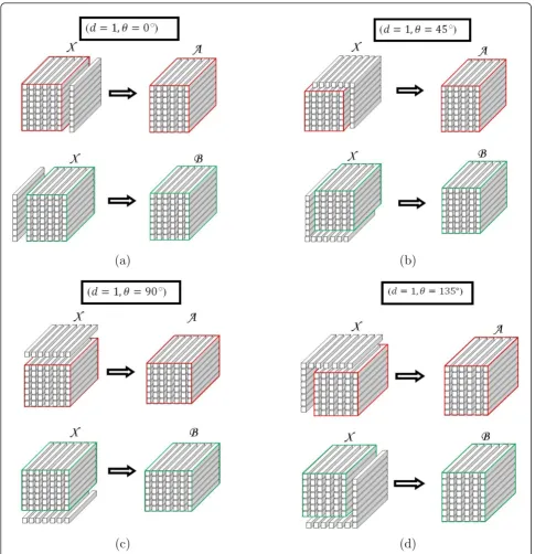
EachP (V,VΔ|d,θ) is the probability that two spectral vectorsVandVΔwith components (i1, ..., ik, ..., in), and (j1, ..., jl, ...,jn) respectively, occur for a given distanced and directionθ(see Figure 2), where n is the number of spectral bands, and (i(k),j(l))ε[1,Ng]2,Ngis the number of gray levels.
Unlike the spatial gray level dependence method in which the estimated second-order joint conditional den-sity functions can be described in a matrix, we propose to represent P (V, VΔ|d, θ) in a structure form of an array Ioccu which is the vector of occurrences and a matrix MV,Vwhich is the matrix ofVandVΔ compo-nents. Each row in the matrix MV,Vcorresponds toV andVΔcomponents. The use of this structure can help us to compute the occurrences while keeping the corre-sponding components vectors ofVand VΔ. For example if we take the first value ofIoccu(i.eIoccu(1)), the corre-sponding components vectors of V and VΔ are in the first row of MV,V (see Figure 3), so Ioccu(1|d, θ) =P(V(1), V(1)|d, θ) where V(1)=MV,V(1, 1 :n)andV(1)=MV,V(1, n+ 1 : 2×n). (1:n): designs columns 1 to n.
In order to compute the matrix MV,V, we define two sub-tensorsA, Bextracted from the tensor dataX for each direction θ as shown in Figure 4. Using the 3-mode flattening matrix ofA,B, we obtain respectively
A3,B3. LetTdenotes the matrix that horizontally con-catenates At
3andBt3, and vertically concatenatesBt3and
At3, whereAt3,Bt3denote the transposed matrices of A3,
B3respectively.Tcan be represented as follows:
T=
At3Bt3 Bt3At3
(1)
The use of this procedure yields us to calculate the spatial and spectral gray level dependence for both θ and (θ+π).
Finally, the matrix MV,Vis obtained by keeping only the rows ofTwith no repetitions, however, the number of repetitions for each row is represented in an array of occurrences calledIoccu. At the end of the process,Ioccu is normalized with respect to the size of MV,V, so that each component represents the probability of occur-rence of a given combination (V, VΔ). The spatial and spectral gray level dependence algorithm can be given as follows:
STEP 1: For a given distance d and angle θ, extract the two sub-tensorsAandBfrom the tensor dataX.
STEP 2:Compute the 3-mode flattening matricesA3,
B3.
STEP 3:Build the matrixT.
STEP 4: Compute MV,Vby keeping only the rowsT with no repetitions.
STEP 5:ComputeIoccu.
2.3. Proposed generalized textures features related to SSGLDM
Haralick texture features comprise 14 features as sum-marized in [1]. However, the most used in literature are energy, entropy, inertia, local homogeneity and correla-tion. In this article we propose seven new generalized texture features.
Suppose that V(k)= (i(1k), i2(k), . . ., i(nk)), and
V(k)= (j(1k), j2(k), . . ., jn(k)), where 1 ≤ k ≤ m, and 1≤m≤N2n
g is the length of the vector of occurrences,
Ngis the number of gray levels andn is the number of bands.
Figure 1Flattening matrices of a third order tensor[52].
Figure 23D representation of the two vectorsVandVΔfor a
given distanced= 1 andθ= 45°.
For convenience,P(V(k), V(k)
|d, θ)will be written as
P(V(k), V(k))in the following equations. Energy:
H= k=m
k=1
P2(V(k), V(k)) (2)
This descriptor is also known as angular second moment or uniformity. In our case, it measures the spa-tial/spectral image homogeneity.
Entropy:
E=− k=m
k=1
P(V(k), V(k))log(P(V(k), V(k))) (3)
The entropy is the counterpart measure of energy. It measures randomness and is smaller for a smooth image than for a coarse image.
(a)
(b)
(c)
(d)
Inertia: ⎧ ⎪ ⎪ ⎨ ⎪ ⎪ ⎩ I= k=m k=1
[V(k)−V(k) ]
2 P(V(k),V(k)
)
where :V(k)−V(k)
2
=
(i(k)1 −j (k) 1)
2
+ (i(k)2 −j (k) 2)
2
+· · ·+ (i(k)n −j(k)n)
2 (4)
This descriptor is also known as contrast or difference moment. It is a measure of image intensity contrast or the spatial/spectral variations present in an image to show the texture fineness.
The inertia value is high when similar spectral vectors are adjacent to each other in the input image and pro-vides a measure of coarseness (similarity).
Local homogeneity:
In= k=m
k=1
1
1 +V(k)−V(k)
2P(V (k), V(k)
) (5)
The local homogeneity or inverse difference moment is a counterpart measure to the contrast descriptor.
Asymmetry:
I= k=m
k=1
[(V(k)−Vx) + (V(k)−Vy)] 3
P(V(k), V(k)) (6)
where:
(V
(k)−
V
x) =
(i
(1k)−
x
1)
2+
· · ·
(i
(nk)−
x
n)
2
(V
(k)−
V
y) =
(j
(1k)−
y
1)
2+
· · ·
(j
(nk)−
y
n)
2
V
x= (x
1,
x
2,
. . .
,
x
n) =
k=mk=1
V
(k)P(V
(k),
V
(k))
V
y= (y1
,
y2
, ...,
y
n) =
k=mk=1
V
(k)P(V
(k),
V
(k))
This descriptor measures the distribution of spectral vectors values around the vectors average using third order statistics.
Proeminence:
I= k=m
k=1
[(V(k)−Vx) + (V(k)−Vy)] 4
P(V(k), V(k)) (7)
This descriptor measures the distribution of spectral vectors values around the vectors average using fourth order statistics.
Correlation:
I= 1 σiσj
k=m
k=1
(V(k)−Vx)(V(k)−Vy)P(V(k), V(k)) (8)
where:
σ2 i =
k=m
k=1
(V(k)−Vx) 2
P(V(k), V(k))
σ2 j =
k=m
k=1
(V(k)−Vy) 2
P(V(k), V(k))
The correlation descriptor measures the linear depen-dency of spectral vectors in the co-occurrence matrix.
In practice, as the number of bands increases, the joint probability P(V(k), V(k)
)decreases. Consequently,
the values of P(V(k), V(k))become nonsignificant which implies a poor overall classification [17,32].
To overcome this issue, we suggest to apply the pro-posed SSGLDM on a subset of bands in the multi-spec-tral image, instead of processing the whole set of bands. The subset of bands can be chosen to remove informa-tion redundancy resulting from highly correlated bands.
2.4. Band selection by minimization of dependent information
In [43], the extraction of selected subsets of spectral image bands can be obtained by means of a criterion based on the minimization of the dependent information (MDI), which consists of a relation between the joint entropy and the union of the conditional entropies of the considered set of image bands. This criterion could be defined by the following expression:
DI=H(A1, . . ., An)− n
i1=1
H(Ai1|Ai2, . . ., Ain) (9)
Where Ai1is a random variable representing the image band i1. Ai2, ...,Ainare the complementary variables of Ai1;H(A1, ...,An)is the joint entropy, which represents the total amount of joint information of set of variables
A1, ..., An; and H(Ai1|Ai2, . . .,Ain)is the conditional entropy that represents the amount of independent information in image band Ai1having measured the rest image bandsAi2, ...,Ain.
This technique behaves as an unsupervised feature selection criterion, providing very satisfactory results with respect to classification accuracy when using the selected bands, even outperforming the other supervised methods used in the comparison in most situations [43]. These performances justify our choice of using MDI [43] for selecting the best relevant bands in the second part of our experiments.
3. Experimental results
extensive experiments are carried out on many multi-spectral images for use in prostate cancer diagnosis. Furthermore, the results of proposed method (SSLGMD) are compared with GLCM, followed by per-formance comparative study and discussion. The second part deals with the curse-of-dimensionality problem. Thus, we extract the best relevant bands of multispectral prostate cancer using MDI technique proposed by Sotoca et al. [43]. Thereafter, we provide some experi-mental results, in order, to see the impact of the selected bands using MDI criterion on the classification accuracy performance using proposed method and GLCM respectively.
3.1. Data set
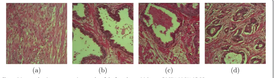
Over the last decade, multi-spectral imagery in pros-tate cancer has become a very useful tool for analyzing and diagnosing pathologies. The prostate cancer is the second most common cancer in men after the skin cancer, and it is also the second in the list of causes for cancer death after the lung cancer. However, the most known method for prostate cancer diagnosis is the prostate-specific antigen (PSA) blood test. In the case of a positive diagnosis, the urologist will often advise a needle biopsy, in which a tiny piece of a tissue is taken from the prostate for analysis [45]. From the analysis, different grades of malignancy correspond to different structural patterns as well as to apparent tex-tures. After the analysis, an experienced pathologist selects the images to reflect the different patterns in prostatic tissues, four major groups usually should be identified (see Figure 5).
●Stroma: STR (normal muscular tissue)
● Benign prostatic hyperplasia: BPH (a benign condition)
●Prostatic intraepithelial neoplasia: PIN (a precursor state for cancer).
● Prostatic carcinoma: PCa (abnormal tissue devel-opment corresponding to cancer).
The data set consists of 624 textured multi-spectral images, of 128 by 128, with each image taken with 16 spectral channels (from 500 to 650 nm) with a 5 nm step [45]. The images were captured using a classical microscope and CCD camera. A liquid crystal tunable filter (LCTF) was inserted in the the optical path between the light source and the chilled CCD camera. The LCTF has a bandwidth accuracy of 5 nm.
The captured images have been chosen to reflect differ-ent grades of malignancy in prostatic tissues and they are labeled into four classes: 176 cases of cancer (Pca), 160 cases of BPH, 144 cases of PIN and 144 cases of Stroma (STR).aThe samples were routinely viewed at prostatic section seen at low power (40x objective magnification) by two highly experimented independent pathologists. The pathologist initially views slides at low power, thereby enabling the location of potentially abnormal regions. Subsequent analysis of these regions at high power enables the histological grading of these areas.
TheX-Yresolution depends on the magnification cho-sen, which is usually high for visualization purposes. In this study, the images of 128 by 128 pixels were cap-tured at anX-Yresolution of 0.12µ/pixel.
Usually, when a biopsy is submitted for analysis, it is very rare that the pathologist finds that the sample is per-fectly normal. There must be at least some benign condi-tion that would explain the high levels of PSA that usually justify needle biopsy. So the main issue is to iden-tify benign from malignant and premalignant conditions.
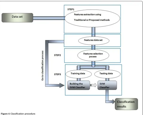
For this purpose, Figure 6 summarizes the different steps used in this article for classification process. The proposed methodology is very important task in prostate cancer diagnosis and could be viewed as a computer-aided system to automatically classify pathological pros-tate images, since each image can be classified into an appropriate class of prostatic tissue.
3.2. Features extraction (Step 1)
The goal of this step of analysis is to characterize the four different groups of multi-spectral images by
(a)
(b)
(c)
(d)
extracting features in order to make classification possible.
All generalized and traditional features mentioned in Sections 3.4 and 3.5 have been used for our experi-ments, and the best performances have been achieved by choosing (d= 1) and the four principal directions (θ = 0°,θ= 45°,θ= 90°, θ= 135°).
We note that, the problem of spatial selection rela-tionships (i.e d and θ) for defining co-occurrence matrices is addressed in [46]. These matrices are maxi-mally reflecting the structure of the underlying texture.
3.3. Features selection for prediction procedure (Step 2)
Feature selection technique is applied to reduce the number of features before applying the classification task. Irrelevant features may have negative effects on a prediction procedure. Moreover, the computational complexity of a classification algorithm may suffer from the curse of dimensionality caused by several features. Features can be selected in many different ways. One
scheme is to select features that correlate strongest to the classification variable.
This has been called maximum-relevance selection. Many heuristic algorithms can be used, such as the sequential forward, backward, or floating selections [42].
On the other hand, features can be selected to be mutually far away from each other, while they still have high correlation to the classification variable. This scheme, termed as minimum-redundancy-maximum-relevance selection [42], has been found to be more powerful than the maximum relevance selection. This justifies the use of this technique in our experiments.
We note that, this technique is not applied when the number of feature is small.
3.4. Classification process (Step 3)
A classification process usually involves trainingand
testing datawhich consist of some data instances. Each instance in the training set contains one“target value” (class labels) and several“attributes”(features).
3.4.1. Using SVM for classification
In [47], several neural networks were compared to the SVM for the classification of hyper-spectral data. The robustness of SVMs was demonstrated and the best results were obtained using a non-linear SVM. In addi-tion, [47] studied Radial Basis Functions (RBF) classifiers and SVM and they noted the favorable behavior of the SVM, from both a theoretical and a practical point of view (see Appendix).
Visually, the images illustrated in Figure 5 are very similar, so the use of SVM for classification issue could be suitable for our applications.
3.5. Results and discussion
The assessment of the classification performance was made using 3-fold cross-validation. Thus, data were randomly splited into 3-sets of a roughly equal size. Splitting was carried out such that the proportion of samples per class was roughly equal across the sets. Each run of the 3-fold cross-validation algorithm con-sisted of a classifier designed on two data subsets (train-ing) while testing was performed on the remaining subset; this is repeated three times. The SVM optimiza-tion was implemented using LIBSVM library through its Matlab interface [48]. The penalty term Cof Gaussian kernel, was fixed to 200 ands2 was selected by using a fivefold cross validation [48]. So that, fivefold cross vali-dation was applied ontraining data in order to estimate s2
which gives the highest classification accuracy rate. Firstly, we compared the performance of SSGLDM with GLCM by the overall classification rate as a criter-ion of the comparison, with reference to a set of images manually classified by experts. Like in the GLCM, in which the co-occurrence matrix is computed for each band, we can apply SSGLDM for each subset of bands in the image. LetSbe a subset of abands in the image (a ≤Nb) where Nbis the number of image bands. For example, if S = (Bl,Bl+1) is a subset of two bands; the SSGLDM can be applied Nb−1 times in the image by varying lfrom 1 toNb−1. Thus, GLCM can be seen as a special case of SSGLDM when S contains only one band.
The number of features is computed for each band in the GLCM, so the total number of features is 7 × (4 directions) × 16 bands = 448. However in the case of SSGLDM, the number of features depends on the choice of subset of bands (S). For example, if S contains two bands, the number of features is 7 ×(4 directions) ×
(Nb −1) bands = 420, where Nb = 16. The minimum redundancy-maximum relevance selection algorithm [42] was used to ensure good classification accuracy by selecting 40 better features from all features generated by SSGLDM.
Table 1 shows the classification results obtained by using SSGLDM, for different subsets of bands (S) for both 32 and 64 gray levels quantification.
It can be clearly observed from Table 1 that the SSGLDM yields better results than the GLCM whenSis less than five bands. Best results are obtained withS= 3
bands, for both 32 and 64 gray levels. However, with 16 bands we obtained a classification accuracy rate around 93%. This may derive from the high correlation of the data. Moreover, as the set of bands increases, the joint probability P(V, VΔ|d, θ) decreases. Consequently, the values of P (V, VΔ|d, θ) become nonsignificant which implies a poor overall classification.
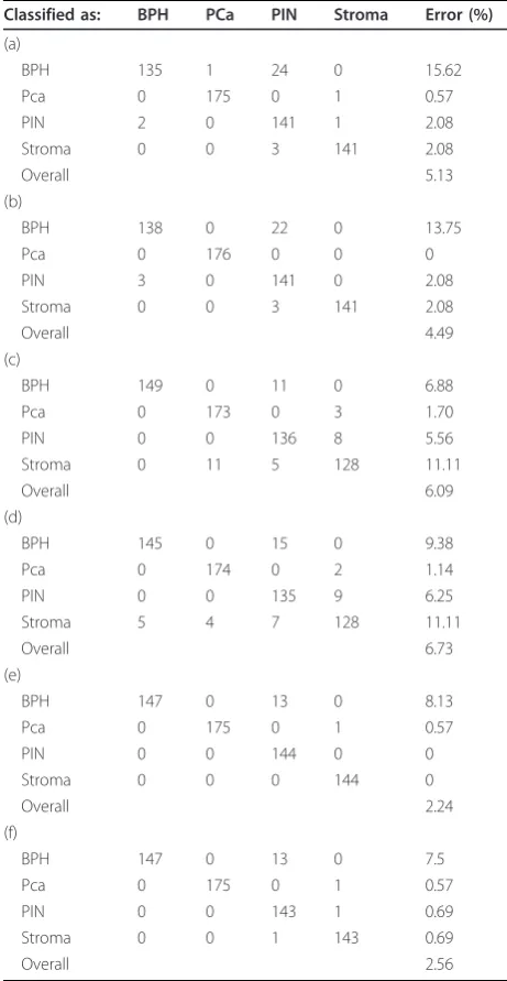
To illustrate the classification of different classes of prostate cancer, we show the confusion matrices obtained by using SSGLDM for different choices ofS. Tables 2a,b depict the results using GLCM (S= 1 band) where Tables 2c,d give the corresponding results using SSGLDM for (S= 16 bands). As can be seen from these tables, the use of SSGLDM with (S = 16) yields worst results in terms of global accuracy rate. However, Tables 2e,f show the achieved improvements when using SSGLDM with (S= 3 bands). Note that in all the cases, BPH and Stroma classes present the highest error rate in terms of classification due to the similarities between two classes; however the use of SSGLDM with (S= 3 bands) reduces significantly the error rate in these classes.
On the other hand, tests of the computation time were performed for the both SSGLDM and GLCM. For this purpose, we used a PCIntel®Core(TM)2 CPU, 2.66 GHz and 3.58 GB Ram. The two methods were imple-mented using Matlab 7.1. Times are given for the com-putation of the co-occurrence matrices and all the features of each method (SSGLDM and GLCM), on images 128 ×128 mentioned in Section 3.1. As shown in on Table 3 The execution time using SSGLDM with (S= 2) is almost the same as GLCM.
Note also that the time keeps growing, when increas-ing the set of bands durincreas-ing the process. However, it decreases for (S = 16), because the SSGLDM was applied just one time for the whole set of spectral bands. Thus, one can conclude that the use SSGLDM with (S = 2) is a quit good compromise between classifi-cation results and computation.
Table 1 Classification results obtained by using the SSGLDM
Subset of bands(S) 1(GLCM) 2 3 4 5 16
Overall classification (%) (32 gray levels)
94.87 97.44 97.76 97.11 96.31 93.91
Overall classification (%) (64 gray levels)
3.5.1. Receiver operating characteristic (ROC)
In order to plot ROC curves, the classifier should be tested using different parameters re-sulting from differ-ent values for false alarm (false positive rate FPR) and sensitivity (true positive rate TPR) rates.
Letπibe the prior probabilities in each classi. In the case of uniform prior probabilities,πican be written as:
∀iπi= N1, where:Nis the number of classes.
Let us suppose a two-class prediction problem (binary classification), in which the outcomes are labeled either as positive (p) or negative (n) class. This is achieved by considering that BPH as the negative diagnosis while PIN and PCa together form the positive diagnosis out-come (the classification of Stroma is relatively simple because of its homogeneous nature at low resolution) [49,50].
Since there are two classes, prior probabilities are linked by the relation:
πpositive= 1−πnegative (10)
ROC curves could be plotted by varying the positive valuesπpositive.
Figure 7 shows a comparative study of the ROC curves using GLCM and SSGLDM respectively, for both 32 and 64 gray levels. Dark, blue and red curves indicate the ROC curves of classified image using SSGLDM (S= 3 bands), GLCM and SSGLDM (S = 16 bands) respec-tively. These results indicate that for all possible values of prior probability πpositive the SSGLDM features with (S= 3) perform better when compared with that derived from GLCM for both 32 and 64 gray levels. The results demonstrate also that our new proposed technique improves ability to distinguish cancer prostate tissues from healthy ones.
However, one can note, that the major issue arise from our proposed method is related to the high dimen-sion of the data and its high correlation. This fact is clearly seen from Table 1 and 2 where classification accuracy is degraded while using SSGLDM with 16 bands. Thus, the main question to be solved is: does the band selection procedure improve the overall classifica-tion rate when using SSGLDM? How would one obtain the optimal number that maximizes classification accu-racy and minimize computational requirements?
In the remainder of this section, we show the influ-ence of selected band method using MDI criterion (Sec-tion 2.4) on the overall classifica(Sec-tion rate by applying the SSGLDM.
3.6. SSGLDM using band selection
In order to exploit inter-band correlation for reducing the multi-spectral band representation, the unsupervised band selection technique by Sotoca et al. [43] has been used to extract the best relevant bands of multispectral prostate cancer database.
All classification rates shown in this section were computed by using 3-fold cross-validation, such as described before.
Table 2 Confusion matrices obtained by using (a) GLCM (32 gray levels), (b) GLCM (64 gray level), (c) SSGLDM (S = 16 bands, 32 gray level), (d) SSGLDM (S= 16 bands, 64 gray level), (e) SSGLDM (S= 3 bands, 32 gray levels), (f) SSGLDM (S= 3 bands, 64 gray levels)
Classified as: BPH PCa PIN Stroma Error (%)
(a)
BPH 135 1 24 0 15.62
Pca 0 175 0 1 0.57
PIN 2 0 141 1 2.08
Stroma 0 0 3 141 2.08
Overall 5.13
(b)
BPH 138 0 22 0 13.75
Pca 0 176 0 0 0
PIN 3 0 141 0 2.08
Stroma 0 0 3 141 2.08
Overall 4.49
(c)
BPH 149 0 11 0 6.88
Pca 0 173 0 3 1.70
PIN 0 0 136 8 5.56
Stroma 0 11 5 128 11.11
Overall 6.09
(d)
BPH 145 0 15 0 9.38
Pca 0 174 0 2 1.14
PIN 0 0 135 9 6.25
Stroma 5 4 7 128 11.11
Overall 6.73
(e)
BPH 147 0 13 0 8.13
Pca 0 175 0 1 0.57
PIN 0 0 144 0 0
Stroma 0 0 0 144 0
Overall 2.24
(f)
BPH 147 0 13 0 7.5
Pca 0 175 0 1 0.57
PIN 0 0 143 1 0.69
Stroma 0 0 1 143 0.69
Overall 2.56
Table 3 Consuming time
Subset of bands 1 (GLCM) 2 3 4 5 16
Note that the same classification procedure used in Section 5.4 was applied for each data cube constructed by the selected bands. However, in the case of SSGLDM the features selection technique [42] was not used because of the small number of features (Figure 6).
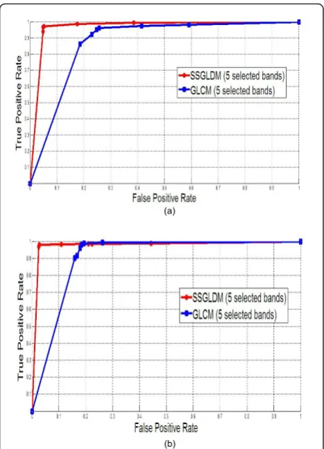
To see the impact of the selected bands using MDI criterion on the classification accuracy performance, we tested the SSGLDM with a variable number of selected bands of multispectral images. Therefore, the plot of Figure 8 shows the result when using 2, 3, 4, 5, 6 and 16 selected bands as input data. A clear improvement of the classification accuracy can be observed by using five selected bands. However, the SSGLDM yields worst results, when more than six selected bands are used. Thus, processing a large number of multispectral bands can result in higher classification inaccuracy than pro-cessing a subset of relevant bands without redundancy.
On the other hand, the classical GLCM provides lower classification accuracy than SSGLDM. However, when more bands selected are used, GLCM performs better. This is mainly due to the use of minimum redundancy-maximum-relevance selection [42] that reduces the number of features and ensure a good classification accuracy.
To gain an insight into the classification of different classes of prostate cancer, the confusion matrices of both SSGLDM and GLCM using five selected bands are also given in Table 4. As can be seen from this table, the use of band selection procedure before applying SSGLDM reduces significantly the error rate in classes and insures a good discrimination power between differ-ent types of tissues.
Figure 9 illustrates the ROC curves obtained with the two methods GLCM and SSGLDM using five selected bands as input data. This clearly demonstrates that our new proposed SSGLDM results in an improved ability to distinguish cancer prostate tissues from healthy ones.
Finally, Table 5 summarizes the processing time for both GLCM and SSGLDM (implemented using Matlab 7.1) versus selected bands. This experiment is conducted on an Intel® Core(TM) 2 CPU, 2.66 GHz and 3.58 GB (a)
(b)
Figure 7The comparative ROC curves.(a)32 gray levels(b)64 gray levels.
(a)
(b)
Ram. As mentioned before, times are given for the com-putation of co-occurrence matrices and all features for each method.
It’s clear from the table that the use of band selection technique reduces significantly the time computation. On the other hand, comparing the results of two meth-ods, SSGLDM ran much faster than the GLCM mainly because SSGLDM features are extracted from the whole data cube of selected bands, unlike the GLDM features which are computed from each selected band.
4. Conclusion
This article describes a new method to generalize the concept of spatial gray level dependence method by assuming the presence of texture joint information between spectral bands. Two ways have been suggested to implement the proposed spatial and spectral gray level dependence method (SSGLDM): (a) applying SSGLDM for each subset of bands in the multi-spectral image; and (b) making a connection between band selection and SSGLDM by using MDI criterion before applying SSGLDM. Extensive experiments have been
carried out on many multi-spectral images for use in prostate cancer diagnosis and quantitative results showed the efficiency of this method compared to the Gray GLCM. SSGLDM has also pro-vided better perfor-mances in terms of classification accuracy and computa-tional complexity. Finally, due to the aspect of this area of research, many issues could be suggested. Open pro-blems that can be investigated in the future include the following:
(1) The new texture characterization method described in this article focuses on second order statis-tics. Therefore, the way forward could be to investigate alternative methods using higher-order statistics.
(2) In this work, the most time consuming task was, by far, the computation of the generalized co-occurrence matrix, which mainly depends on spectral vector-pairs distances and a large numbers of spectral bands. The Table 4 Confusion matrices obtained by using (a) GLCM
(5 selected bands, 32 gray levels), (b) SSGLDM (5 selected bands, 32 gray levels), (c) GLCM (5 selected bands, 64 gray levels), (d) SSGLDM (5 selected bands, 64 gray levels)
Classified as: BPH PCa PIN Stroma Error (%)
(a)
BPH 147 0 13 0 8.13
Pca 0 174 2 0 1.14
PIN 2 12 129 1 10.42
Stroma 9 0 1 134 6.94
Overall 6.41
(b)
BPH 148 0 12 0 7.5
Pca 0 174 2 0 1.14
PIN 2 11 130 1 9.72
Stroma 1 0 1 142 1.39
Overall 4.81
(c)
BPH 141 0 15 4 11.88
Pca 0 175 1 0 0.57
PIN 0 13 130 1 9.72
Stroma 17 0 1 126 12.5
Overall 8.33
(d)
BPH 149 0 11 0 6.88
Pca 0 176 0 0 0
PIN 2 10 131 1 9.03
Stroma 0 0 1 143 0.69
Overall 4.01
(a)
(b)
Figure 9The comparative ROC curves using five selected bands as input data.(a)32 gray levels(b)64 gray levels.
Table 5 Computation time
Number of selected bands 2 3 4 5 6
nature of the calculation makes it suitable for parallel processing because the same calculations are performed on successive image blocks.
(3) The generalized multi-band texture method is pro-posed in this article to solve the characterization of multi-band texture images problem. Medical data sets that use multi-spectral data have been used to evaluate our proposed algorithm. In future, to apply our pro-posed algorithms to other applications such as hyper-spectral satellite imagery or skin cancer detection.
Endnote
a
The data set used in this study were provided from Pathology department team at Queen’s university of Bel-fast under the direction of Prof. Hamilton.
Appendix
Support vector machines (SVM)
The aim of SVM is to produce a model (based on the training data) that predicts target value of data instances in the testing set which are given only by the attributes. Given a labeled training data set {(x1, y1), ..., (xn, yn)}, wherexiÎℝnandyiÎ{−1, 1}, the SVM [47,51] require the solution of the following optimization problem:
min w,ξi,b
1 2w
2+C
i ξi
(:1)
constrained to:
yi(φ(xi), w+b)≥1−ξi∀i= 1, . . ., n
ξi≥0 ∀i= 1, . . ., n (:2)
where〈.,.〉: is the inner product.
In the case of a nonlinear classification of samples, the training vectorsxiare mapped into a higher (maybe infi-nite) dimensional space by the function, wis the vec-tor of hyperplane coefficients (orientation), b is a bias term. The regularization parameter Ccontrols the gen-eralization capabilities of the classifier and it must be selected by the user, and ξiare positive slack variables enabling to deal with permitted errors. The decision function is found by solving the convex optimization problem max αi ⎧ ⎨ ⎩ i αi−
1 2
i,j
αiαjyiyjφ(xi),φ(xj)
⎫ ⎬
⎭ (:3)
subject to:
0≤αi≤C
i α
iyi= 0 i= 1, ...,n (:4)
whereaiare the Lagrange coefficients. It is worth not-ing that allmappings used in the SVM learning occur in the forme of inner product. This allows us to define the classical Gaussian kernelKsgiven by this formula:
kσ(xi, xj) =φ(xi), φ(xj)
=
exp
−xi−xj 2
2σ2
(:5)
where the norm is the Euclidean norm ands Î ℝ+ tunes the flexibility of the kernel. The classification of a sample × is achieved by looking to which side of the hyperplane it belongs
f(x) = sgn
n
i=1
yiαikσ(xi, x) +b
(:6)
Whereb can be used for computingai.
The SVMs are mainly a nonparametric method, yet some parameters need to be tuned before the optimiza-tion. In the case of Gaussian kernel, there are two para-meters: C, which is the penalty term, and s, which is the width of the exponential.
Acknowledgements
I would to acknowledge contribution from Dr. MA Roula and the Pathology department team at the Queen’s university of Belfast under the direction of Prof. Hamilton for kindly providing maging data used in this study.
Competing interests
The authors declare that they have no competing interests.
Received: 8 September 2011 Accepted: 29 May 2012 Published: 29 May 2012
References
1. RM Haralick, K Shanmugam, IH Dinstein, Textural features for image classification. IEEE Trans Syst Man Cybern.SMC-3(6), 610–621 (1973) 2. LK Soh, C Tsatsoulis, Texture analysis of SAR sea ice imagery using gray
level co-occurrence matrices. IEEE Trans Geosci Remote Sens.GeoRS-37(2), 780–795 (1999)
3. M Do, M Vetterli, Wavelet-based texture retrieval using generalized gaussian density and kullback-leibler distance. IEEE Trans Image Process.IP 11(2), 146–158 (2002)
4. G Hazel, Multivariate gaussian MRF for multispectral scene segmentation and anomaly detection. IEEE Trans Geosci Remote Sens.GeoRS 38(2), 1199–1211 (2000)
5. S Derrode, G Mercier, JM LeCaillec, R Garello, Estimation of sea ice SAR clutter statistics from Pearson’s system of distributions, inInternational Geoscience and Remote Sensing Symposium (IGARSS’01), Sydney, Australia,1, 190–192 (2001)
6. C Munzenmayer, H Volk, C Kublbeck, K Spinnler, T Wittenberg, Multispectral texture analysis using interplane sum and difference histograms,Procs DAGM Symp, Zurich, Switzerland, (Springer, 2002), pp. 25–31
7. JA Benediktsson, M Pesaresi, K Arnason, Classification and feature extraction for remote sensing images from urban areas based on morphological transformations. IEEE Trans Geosci Remote Sens.41(9), 1940–1949 (2003). doi:10.1109/TGRS.2003.814625
9. O Rajadell, P Garca-Sevilla, F Pla, Textural features for hyperspectral pixel classification, inproceedings of the 4th Iberian Conference on Pattern Recognition and Image Analysis, Póvoa de Varzim, Portugal, 208–216 (2009) 10. G Rellier, X Descombesm, F Falzon, J Zerubia, Texture feature analysis using
a gauss-Markov model in hyperspectral image classification. IEEE Trans Geosci Remote Sens.42(7), 1543–1551 (2004)
11. A Rosenfeld, CY Wang, AY Wu, Multispectral texture. IEEE Trans Syst Man Cyber-net.SMC-12(1), 79–84 (1982)
12. S Sarkar, G Healey, Hyperspectral texture classification using generalized Markov fields. IEEE Comput Soc Conf Comput Vis Pattern Recog.43(2), 3038–3044 (2004)
13. L Lepisto, I Kunttu, J Autio, A Visa, Classification method for colored natural textures using gabor filtering, in12th International Conference on Image Analysis and Processing, Mantova, Italy, 397–401 (2003)
14. V Arvis, C Debain, M Berducat, A Benassi, Generalization of the cooccurrence matrix for colour images: application to colour texture classification. Image Anal Stereol.23, 63–73 (2004). doi:10.5566/ias.v23.p63-72
15. M Hauta-Kasari, J Parkkinen, T Jaaskelainen, R Lenz, Generelized cooccurrence matrix for multispectral texture analysis,Proceedings of the 13th International Conference on pattern Recognition, ICPR’96, Vienna, Austria,
2, 785–789 (1996)
16. R Khelifi, M Adel, S Bourennane, Texture classification for multi-spectral images using spatial and spectral gray level differences, inIEEE International Conference on Image Processing Theory, Tools and Applications, IPTA’10, Paris, France, 330–333 (2010)
17. R Khelifi, M Adel, S Bourennane, Generalized gray level dependence method for prostate cancer classification, inIEEE International Workshop on Systems, Signal Processing and their Applications (WOSSPA), Tipaza, Algeria, 295–298 (2011)
18. L Lepisto, I Kunttu, J Autio, A Visa, Rock image classification using non-homogeneous textures and spectral imaging, inInternational Conference in Central Europe on Computer Graphics, Visualization and Computer Vision, Plzen, Czech Republic, 82–86 (2003)
19. F Tsai, CK Chang, JY Rau, TH Lin, GR Liu, 3D computation of gray level co-occurrence in hyperspectral image cubes. inProceedings of the 6th international conference on Energy minimization methods in computer vision and pattern recognition.4679, 429–440 (2007). doi:10.1007/978-3-540-74198-5_33
20. M Fauvel, JA Benediktsson, J Chanussot, JR Sveinsson, Spectral and spatial classification of hyperspectral data using svms and morphological profiles. IEEE Trans Geosci Remote Sens.46(11), 3804–3814 (2008)
21. JA Palmason, JA Benediktsson, JR Sveinsson, J Chanussot, Classification of hyperspectral data from urban areas using morphological preprocessing and independent component analysis, inGeoscience and Remote Sensing Symposium, Seoul, Korea, 176–179 (2005)
22. A Plaza, P Martinez, R Perez, J Plaza, Spatial/spectral endmember extraction by multidimensional morphological operations. IEEE Trans Geosci Remote Sens.40(9), 2025–2041 (2002). doi:10.1109/TGRS.2002.802494
23. A Puissant, J Hirsch, C Weber, The utility of texture analysis to improve per-pixel classification for high to very high spatial resolution imagery. Int J Remote Sens.26(4), 733–745 (2005). doi:10.1080/01431160512331316838 24. D Claussi, An analysis of co-occurrence texture statistics as a function of
grey level quantization. Can J Remote Sens.28(1), 45–62 (2002). doi:10.5589/m02-004
25. J Kiema, Texture analysis and data fusion in the extraction of topographic objects from satellite imagery. Int J Remote Sens.23(4), 767–776 (2002). doi:10.1080/01431160010026005
26. T Bau, G Healey, Rotation and scale invariant hyperspectral classification using 3D Gabor filters. Proc SPIE Int Soc Opt Eng.7334(15),
73340B–73340B-13 (2009)
27. A Jaim, G Healey, A multiscale representation including oppponent color features for texture recognition. IEEE Trans Image Process.7(1), 124–128 (1998). doi:10.1109/83.650858
28. M Shi, G Healey, Hyperspectral texture recognition using a multiscale opponent representation. IEEE Trans Geosci Remote Sens.41(5), 1090–1095 (2003). doi:10.1109/TGRS.2003.811076
29. MP Dubuisson-Jolly, A Gupta, Color and texture fusion: application to aerial image segmentation and GIS updating. Image Vis Comput.18(10), 823–832 (2000). doi:10.1016/S0262-8856(99)00050-5
30. C Palm, Color texture classification by integrative co-occurrence matrices. Pattern Recog.37(5), 965–976 (2004). doi:10.1016/j.patcog.2003.09.010 31. M Mirmehdi, M Petrou, Segmentation of color textures. IEEE Trans Pattern
Anal Mach Intell.22(2), 142–159 (2000). doi:10.1109/34.825753 32. R Khelifi, M Adel, S Bourennane, Spatial and spectral dependence
co-occurrence method for multi-spectral image texture classification, inIEEE International Conference on Image Processing, Hong Kong, China, 917–9200 (2010)
33. P Bajcsy, P Groves, Methodology for hyperspectral band selection. Photogram Eng Remote Sens J.10, 793–802 (2004)
34. JA Benediktsson, JR Sveinsson, K Amason, Classification and feature extraction of AVIRIS data. IEEE Trans Geosci Remote Sens.33(5), 1194–1205 (1995). doi:10.1109/36.469483
35. G Hughes, On the mean accuracy of statistical pattern recognizers. IEEE Trans Inf Theory.14(1), 55–63
36. D Landgrebe, Hyperspectral image data analysis as a high dimensiona. IEEE Signal Process Mag.19(1), 17–28 (2002). doi:10.1109/79.974718
37. EM Bassettm, SS Shen, Information theory-based band selection for multispectral systems. Proc SPIE.3118, 28–35 (1997)
38. CI Chang, Q Du, TL Sun, LG Althouse, A joint band prioritization and band-decorrelation approach to band selection for Hyperspectral image classification. IEEE Trans Geosci Remote Sens.37(6), 2631–2641 (1999). doi:10.1109/36.803411
39. H Du, H Qi, X Wang, WE Snyder, Band selection using independent component analysis for Hyperspectral image processing, inProceedings of 32nd Applied Imagery Pattern Recognition Workshop, Washington DC, 93–98 (2003)
40. JM Sotoca, F Pla, AC Klaren, Unsupervised band selection for Multispectral images using information theory, inProceedings of International Conference on Pattern Recognition, (Cambridge, UK, 2004), pp. 510–513
41. H Wang, E Angelopoulou, Sensor band selection for multispectral imaging via average normalized information. J Real-Time Image Process.1(2), 109–121 (2006). doi:10.1007/s11554-006-0014-9
42. H Peng, F Long, C Ding, Feature selection based on mutual information: criteria of max-dependency, max-relevance, and min-redundancy. IEEE Trans Pattern Anal Mach Intell.27(8), 1226–1238 (2005)
43. JM Sotoca, F Pla, JS Sanchez, Band selection in multispectral images by minimization of dependent information. IEEE Trans Syst Man Cybern Part C Appl Rev.37(2), 258–267 (2007)
44. D Letexier, S Bourennane, JB Talon, Nonorthogonal tensor matricization for hyper-spectral image filtering. IEEE Geosci Remote Sens Lett.5(1), 3–7 (2008)
45. JN Eble, DG Bostwick,Urologic Surgical Pathology, (MO: Mosby-Year Book, St. Louis, Inc., 1996), pp. 291–294
46. SH Zucker, D Terzopoulosand, Finding structure in co-occurrence matrices for texture analysis, computer graphics and image processing. Comput Graph Image Process.12(3), 286–308 (1980). doi:10.1016/0146-664X(80) 90016-7
47. G Camps-Valls, L Gomez-Chova, J Munoz-Mari, J Vila-Frances, J Calpe-Maravilla, Composite kernels for hyperspectral image classification. IEEE Geosci Remote Sens Lett.3(1), 93–97 (2006). doi:10.1109/LGRS.2005.857031 48. CC Chang, CJ Lin, LIBSVM: a library for support vector machines. Software
available at http://www.csie.ntu.edu.tw/~cjlin/libsvm
49. S Bouatmane, MA Roula, A Bouridane, S Al-Maadeed, Round-Robin sequential forward selection algorithm for prostate cancer classification and diagnosis using multispectral imagery,J Mac Vis Appl, Vol. 1(1) (Springer Verlag, 2010), pp. 1–14
50. MA Roula, Machine vision and texture analysis for the automated identification of tissue patterns in prostatic neoplasia. Ph.thesis D, (Queens University of Belfast 2004)
51. C Cortes, V Vapnik, Support-vector networks. Mach Learn.20(3), 273–297 (1995)
52. D Letexier, S Bourennane, Multidimensional wiener filtering using fourth order statistics of hyperspectral images, inIEEE International Conference on Acoustics, Speech and Signal Processing, Las Vegas, Nevada, USA, 917–920 (2008)
doi:10.1186/1687-6180-2012-118
Cite this article as:Khelifiet al.:Multispectral texture characterization: application to computer aided diagnosis on prostatic tissue images.
![Figure 1 Flattening matrices of a third order tensor [52].](https://thumb-us.123doks.com/thumbv2/123dok_us/1140932.1143163/3.595.57.291.89.234/figure-flattening-matrices-order-tensor.webp)