R E S E A R C H
Open Access
Decentralized estimation over orthogonal
multiple-access fading channels in wireless sensor
networks
–
optimal and suboptimal estimators
Xin Wang
*and Chenyang Yang
Abstract
We study optimal and suboptimal decentralized estimators in wireless sensor networks over orthogonal multiple-access fading channels in this paper. Considering multiple-bit quantization for digital transmission, we develop maximum likelihood estimators (MLEs) with both known and unknown channel state information (CSI). When training symbols are available, we derive a MLE that is a special case of the MLE with unknown CSI. It implicitly uses the training symbols to estimate CSI and exploits channel estimation in an optimal way and performs the best in realistic scenarios where CSI needs to be estimated and transmission energy is constrained. To reduce the computational complexity of the MLE with unknown CSI, we propose a suboptimal estimator. These optimal and suboptimal estimators exploit both signal- and data-level redundant information to combat the observation noise and the communication errors. Simulation results show that the proposed estimators are superior to the existing approaches, and the suboptimal estimator performs closely to the optimal MLE.
Keywords:Decentralized estimation, maximum likelihood estimation, fading channels, wireless sensor network
1 Introduction
Wireless sensor networks (WSNs) consist of a number of sensors deployed in a field to collect information, for example, measuring physical parameters such as tem-perature and humidity. Since the sensors are usually powered by batteries and have very limited processing and communication abilities [1], the parameters are often estimated in a decentralized way. In typical WSNs for decentralized estimation, there exists a fusion center (FC). The sensors transmit their locally processed obser-vations to the FC, and the FC generates the final estima-tion based on the received signals [2].
Both observation noise and communication errors deteriorate the performance of decentralized estimation. Traditional fusion-based estimators are able to minimize the mean square error (MSE) of the parameter estima-tion by assuming perfect communicaestima-tion links (see [3] and references therein). They reduce the observation noise by exploiting the redundant observations provided by multiple sensors. However, their performance
degrades dramatically when communication errors can-not be ignored or corrected. On the other hand, various wireless communication technologies aiming at achiev-ing transmission capacity or improvachiev-ing reliability do not minimize the MSE of the parameter estimation. For example, although diversity combining reduces the bit error rate (BER), it requires that the signals transmitted from multiple sensors are identical, which is not true in the context of WSNs due to the observation noise at sensors. This motivates to optimize estimator at the FC under realistic observation and channel models, which minimizes the MSE of parameter estimation.
The bandwidth and energy constraints are two critical issues for the design of WSNs. When the strict band-width constraint is taken into account, the decentralized estimation when the sensors only transmit one bit for each observation, that is, using binary quantization, is studied in [4-9]. When communication channels are noiseless, a maximum likelihood estimator (MLE) is introduced and optimal quantization is discussed in [4]. A universal and isotropic quantization rule is proposed in [6], and adaptive binary quantization methods are studied in [7,8]. When channels are noisy, the MLE in * Correspondence: [email protected]
School of Electronics and Information Engineering, Beihang University, Beijing 100191, China
additive white Gaussian noise (AWGN) channels is stu-died and several low complexity suboptimal estimators are derived in [9]. It has been found that the binary quantization is sufficient for decentralized estimation at low observation signal-to-noise ratio (SNR), but more bits are required for each observation at high observa-tion SNR [4].
When the energy constraint and general multi-level quantizers are considered, various issues of the decen-tralized estimation are studied under different channels. When communications are error free, the quantization at the sensors is designed in [10-12]. The optimal trade-off between the number of active sensors and the quan-tization bit rate of each sensor is investigated under total energy constraint in [13]. In binary symmetrical channels (BSCs), the power scheduling is proposed to reduce the estimation MSE when the best linear unbiased estimator (BLUE) and a quasi-BLUE, where quantization noise is taken into account, are used at the FC [14]. Nonetheless, to the best of the authors’ knowl-edge, the optimal decentralized estimator using multi-ple-bit quantization in fading channels is still unavailable. Although the MLE proposed in AWGN channels [9] can be applied for fading channels if the channel state information (CSI) is known at the FC, it only considers binary quantization.
Besides the decentralized estimation based on digital communications, the estimation based on analog com-munications receives considerable attentions due to the important conclusions drawn from the studies for the multi-terminal coding problem [15,16]. The most popu-lar scheme is amplify-and-forward (AF) transmission, which is proved to be optimal in quadratic Gaussian sensor networks under multiple-access channels (MACs) with AWGN [17]. The power scheduling and energy efficiency of AF transmission are studied under AWGN channels in [18], where AF transmission is shown to be more energy efficient than digital communications. However, in fading channels, AF transmission is no longer optimal in orthogonal MACs [19-21]. The outage laws of the estimation diversity with AF transmission in fading channels are studied in [20] and [21] in different asymptotic regimes. These studies, especially the results in [19], indicate that the separate source-channel coding scheme is optimal in fading channels with orthogonal multiple-access protocols, which outperforms AF trans-mission, a simple joint source-channel coding scheme.
In this paper, we develop optimal and suboptimal decentralized estimators for a deterministic parameter considering digital communication. The observations of the sensors are quantized, coded and modulated, and then transmitted to the FC over Rayleigh fading ortho-gonal MACs. Because the binary quantization is only
applicable at low observation SNR levels [4,13], a gen-eral multi-bit quantizer is considered.
We strive for deriving MLEs and feasible suboptimal estimator when different local processing and communi-cation strategies are used. To this end, we first present a general message function to represent various quantiza-tion and transmission schemes. We then derive the MLE for an unknown parameter with known CSI at the FC.
In typical WSNs, the sensors usually cannot transmit too many training symbols for the receiver to estimate channel coefficients because of both energy and band-width constraints. Therefore, we will consider realistic scenarios that the CSI is unknown at the FC when no or only a few training symbols are available. It is known that channel information has a large impact on the structure and the performance of decentralized estima-tion. In orthogonal MACs, most of the existing works assume that perfect CSI is available at the FC. Recently, the impact of channel estimation errors on the decen-tralized detection in WSNs is studied in [22], and its impact on the decentralized estimation when using AF transmission is investigated in [23]. However, the decen-tralized estimation with unknown CSI for digital com-munications has still not been well understood.
Our contributions are summarized as follows. We develop the decentralized MLEs with known and unknown CSI at the FC over orthogonal MACs with Rayleigh fading. The performance of the MLE with known CSI can serve as a practical performance lower bound of the decentralized estimation, whereas the MLE with unknown CSI is more realistic. For the spe-cial cases of error-free communications or noiseless observations, we show that the MLEs degenerate into the well-known centralized fusion estimator–BLUE–or a maximal ratio combiner (MRC)-based estimator when CSI is known and a subspace-based estimator when CSI is unknown. This indicates that our estima-tors exploit both data-level redundancy and signal-level redundancy provided by multiple sensors. To provide feasible estimator with affordable complexity, we pro-pose a suboptimal algorithm, which can be viewed as a modified expectation-maximization (EM) algorithm [24].
2 System model
We consider a typical kind of WSNs that consists ofN sensors and a FC to measure an unknown deterministic parameterθ, where there are no inter-sensor communi-cations among the sensors. The sensors process their observations for the parameterθbefore transmission. For digital communications, the processing includes quanti-zation, channel coding and modulation. For analog com-munications, the processing may simply be amplifying the observations before transmission. A messaging func-tionc(x) is used to describe the local processing. Though we can usec(x) for both digital and analog communica-tion systems, we focus on digital transmission since the popular analog transmission scheme, AF, has been shown to be not optimal in fading channels [19-21].
2.1 Observation model
The observation for the unknown parameter provided by theith sensor is
xi=θ+ns,i, i= 1,. . .,N, (1)
wherens, iis the independent and identically
distribu-ted (i.i.d.) Gaussian observation noise with zero mean and variance σs2, and θ is bounded within a dynamic range [-V, +V].
2.2 Quantization, coding, and modulation
We use the messaging function c(x)|ℝ ®ℂLto repre-sent all the processing at the sensors including quantiza-tion, coding and modulaquantiza-tion, which maps the observations to the transmit symbols. To facilitate analy-sis, the energy of the transmit symbols is normalized to 1, that is,
c(x)Hc(x) = 1, ∀x∈R. (2)
We consider uniform quantization by regardingθas a uniformly distributed parameter. Uniform quantization is the Lloyd-Max quantizer that minimizes the quantiza-tion distorquantiza-tion of uniformly distributed sources [25,26]. For an M-level uniform quantizer, define the dynamic range of the quantizer as [-W, +W], and then all the possible quantized values of the observations can be written as
Sm=m−W, m= 0,. . .,M−1, (3)
whereΔ= 2W/(M- 1) is the quantization interval. The observations are rounded to the nearest Sm, so
thatc(x) is a piecewise constant function described as
c(x) =
⎧ ⎨ ⎩
c0,
cm,
cM−1,
−∞<x≤S0+ 2 Sm−2 <x≤Sm+2
SM−1−2 <x<+∞
, (4)
where cm = [cm,1, ..., cm, L]T is the Lsymbols
corre-sponding to the quantized observationSm,m= 0, ...,M
- 1.
Under the assumption thatWis much larger than the dynamic range ofθ, the probability that |xi|>Wcan be
ignored. Then,c(x) is simplified as
c(x) =cm, Sm−
2 <x≤Sm+
2. (5)
Define the transmission codebook as
Ct= [c0,. . .,cM−1]∈CL×M, (6)
which can be used to describe any coding and modu-lation scheme following theM-level quantization.
The sensors can use various codes such as natural binary codes to represent the quantized observations. In this paper, our focus is to design decentralized estima-tors; therefore, we will not address the transmission codebook optimization for parameter estimation.
2.3 Received signals
Since we consider orthogonal MACs, the FC can per-fectly separate and synchronize to the received signals from different sensors. Assume that the channels are block fading, that is, the channel coefficients are invar-iant during the period that the sensors transmit L sym-bols representing one observation. After matched filtering and symbol-rate sampling, theLreceived sam-ples corresponding to the L transmitted symbols from theith sensor can be expressed as
yi=Edhic(xi) +nc,i, i= 1,. . .,N, (7)
whereyi= [yi,1, ...,yi, L]T, hiis the channel coefficient,
which is i.i.d. and subjected to complex Gaussian distri-bution with zero mean and unit variance, nc, iis a
vec-tor of thermal noise at the receiver subjecting to complex Gaussian distribution with zero mean and cov-ariance matrixσ2
cI, andEdis the transmission energy for
each observation.
3 Optimal estimators with or without CSI
In this section, we derive MLEs when CSI is known or unknown at the receiver of the FC, respectively. To understand how they deal with both the communication errors and the observation noises, we study two special cases. The MLE using training symbols in the transmis-sion codebook is also studied as a special form of the MLE with unknown CSI.
3.1 MLE with known CSI
logp(Y|h,θ) =
N
i=1
logp(yi|hi,θ)
= N i=1 log ⎛ ⎝ +∞ −∞
p(yi|hi,x)p(x|θ)dx
⎞ ⎠,
(8)
where Y= [y1, ...,yN],h = [h1, ...,hN] T
is the channel coefficients vector, andp(x|θ) is the conditional prob-ability density function (PDF) of the observation givenθ. Following the observation model shown in (1), we have
p(x|θ) = √ 1 2πσs
exp
−(x−θ)2 2σ2
s
. (9)
According to the received signal model shown in (7), the PDF of the received signals given CSI and the obser-vation of the sensors is
p(yi|hi,x) =
1 (πσ2
c)
Lexp
−yi−
√
Edhic(x)22
σ2
c
,(10)
where ||z||2= (zHz)1/2isl2 norm of vectorz.
Substituting (9) and (10) into (8), we obtain the log-likelihood function for estimating θ, which can be used for any messaging function c(x), no matter when it describes analog or digital communications.
For digital communications, c(x) is a piecewise con-stant function as shown in (4). To simplify the analysis, we use its approximate form shown in (5) in the rest of this paper. After substituting (5) into (10) and then to (8), we have
logp(Y|h,θ) =
N
i=1
log
M−1
m=0
p(yi|hi,cm)p(Sm|θ)
,(11)
where p(yi|hi,cm) is the PDF of the received signals
given the CSI and the transmitted symbols of the sen-sors, which is
p(yi|hi,cm) =
1 (πσ2
c)
Lexp
−yi−
√
Edhicm22
σ2
c
,(12)
andp(Sm|θ) is the probability mass function (PMF) of
the quantized observation givenθ, which is
p(Sm|θ) = Q
Sm− 2 −θ
σs
−Q
Sm+2 −θ
σs
,(13)
whereQ(x) = √1
2π
∞
x exp
−t2
2
dt.
The MLE is obtained by maximizing the log-likelihood function shown in (11).
3.1.1 Special case whenσ2
s →0
When the observation SNR tends to infinity, the obser-vations of the sensors are perfect, that is, xi=θ,∀i= 1,
...,N. The PDF of the observationxigivenθdegrades to
p(x|θ) =δ(x−θ), (14)
whereδ(x) is the Dirac-delta function.
In this case, the log-likelihood function for both ana-log and digital communications has the same form, which can be obtained by substituting (14) into (8). After ignoring all terms that do not affect the estima-tion, the log-likelihood function is simplified as
logp(Y|h,θ) =−
N
i=1
yi−√Edhic(θ)22
σ2
c
, (15)
wherec(θ) is the transmitted symbols when the obser-vations of the sensors areθ.
For digital communications,c(θ) is a code word of Ct
and is a piecewise constant function. Therefore, we can-not getθby taking partial derivative of (15). Instead, we first regard c(θ) as the parameter to be estimated and obtain the MLE for estimatingc(θ). Then, we use it as a decision variable to detect the transmitted symbols and reconstruct θaccording to the quantization rule with the decision results.
The log-likelihood function in (15) is concave with respect to (w.r.t.) c(θ), and its only maximum is obtained by solving the equation∂logp(Y|h, θ)/∂c(θ) = 0, which is
ˆ
c(θ) = √ 1 Ed
N j=1|hi|2
N
i=1
h∗iyi. (16)
It follows that when the observations are perfect, the structure of the MLE is the MRC concatenated with data demodulation and parameter reconstruction. This is no surprise since in this case, all the signals trans-mitted by different sensors are identical; thus, the recei-ver at the FC is able to apply the conventional direcei-versity technology to reduce the communication errors.
3.1.2 Special case whenσ2
c →0
When the communications are perfect, yi=√Edhicmi. It
means that yi merely depends oncmior equivalently
depends on Smi. Then, the log-likelihood function
becomes a function of the quantized observationSmi.
The log-likelihood function with perfect communica-tions becomes
logp(Y|h,θ)→logp(S|h,θ) =
N i=1 log Q Smi−2−θ
σs
−Q
Smi+2−θ σs
whereS= [Sm1,. . .,SmN]
T.
By taking the derivative of (17) to be 0, we obtain the likelihood equation N i=1 exp
−(Smi−2−θ)
2
2σ2
s
−exp
−(Smi−2−θ)
2
2σ2
s
Q
(Smi−2−θ)
σs
−Q
(Smi−2−θ)
σs
= 0.(18)
Generally, this likelihood equation has no closed-form solution. Nonetheless, the closed-form solution can be obtained when the quantization noise is very small, that is, Δ ® 0. Under this condition, Smi →xi and (18)
becomes
lim
→0
∂logp(S|h,θ)
∂θ =
N
i=1 xi−θ
σ2
s
= 0. (19)
The MLE obtained from (19) is
ˆ θ = 1
N
N
i=1
xi. (20)
It is also no surprise to see that the MLE reduces to BLUE, which is often applied in centralized estimation [14], where the FC can obtain all raw observations of the sensors.
3.2 MLE with unknown CSI
In practical WSNs, the FC usually has no CSI, and the sensors can transmit training symbols to facilitate chan-nel estimation. The training symbols can be incorpo-rated into the message function c(x). Then, the MLE with training symbols available is a special form of the MLE with unknown CSI. We will derive the MLE with unknown CSI with general c(x) in the following and derive that with training symbols in c(x) in next subsection.
When CSI is unknown at the FC, the log-likelihood function is
logp(Y|θ) =
N i=1 ⎛ ⎝log ⎛ ⎝ +∞ −∞
p(yi|x)p(x|θ)dx ⎞ ⎠ ⎞ ⎠, (21)
which has a similar form to the likelihood function with known CSI shown in (8).
According to the received signal model, given x, yi
subjects to zero mean complex Gaussian distribution, that is,
p(yi|x) = 1 πLdetR
y
exp(−yHi R−y1yi), (22)
whereRy is the covariance matrix ofyi, which is
Ry=σc2I+Edc(x)c(x)H. (23)
Since the energy of the transmit symbols is normal-ized as shown in (2), we have
Ryc(x) = (σc2I+Edc(x)c(x)H)c(x)
= (σc2+Ed)c(x).
(24)
Therefore,c(x) is an eigenvector of Ry, and the corre-sponding eigenvalue is(σ2
c +Ed).
For any vector orthogonal toc(x), denoted asc⊥(x), we have
Ryc⊥(x) =
σ2
cI+Edc(x)c(x)H
c⊥(x)
=σc2c⊥(x).
(25)
Therefore, the eigenvalues corresponding to the remainingL- 1 eigenvectors are allσ2
c. The determinant
ofRyis
detRy= (Ed+σc2)σ
2(L−1)
c . (26)
Following the Matrix Inversion Lemma [27], we have
R−y1= 1 σ2
c
I− Ed
σ2
c(Ed+σc2)
c(x)c(x)H. (27)
Substituting (26) and (27) into (22), we have
p(yi|x) =αexp
−yi22
σ2
c
+Edy
H
i c(x)c(x)
H yi
σ2
c(Ed+σc2)
=αexp
−yi22
σ2
c
+ Ed|y
H
i c(x)|2
σ2
c(Ed+σc2)
,
(28)
whereais a constant.
Upon substituting (28) and (9) into (21), the log-likeli-hood function becomes
logp(Y|θ) =
N i=1 log ⎛ ⎝ +∞ −∞ exp
−(x−θ) 2
2σ2
s
−yi22 σ2
c
+Ed|y H
ic(x)|2
σ2
c(Ed+σc2)
dx ⎞ ⎠. (29)
Then the MLE is obtained as
ˆ
θ = arg max
θ logp(Y|θ). (30)
When considering digital communications, by substi-tuting (5) into (29), the log-likelihood function is obtained as
logp(Y|θ) =
N i=1 log M m=1
p(yi|cm)p(Sm|θ)
wherep(Sm|θ) is shown in (13), and
p(yi|cm) =αexp
−yi22
σ2
c
+ Ed|y
H
i cm|2
σ2
c(Ed+σc2)
. (32)
3.2.1 Special case whenσ2
s →0
Similarly to the log-likelihood function with known CSI, the log-likelihood function with unknown CSI for per-fect observations has the same form for both analog and digital communications.
Upon substituting (14) into (21) and ignoring all terms that do not affect the estimation, the log-likelihood function becomes
logp(Y|θ) =
N
i=1
|yHi c(θ)|2
= c(θ)H
N
i=1 yiyHi
c(θ).
(33)
Again, sincec(θ) is underivable for digital communica-tions, we regard c(θ) as the parameter to be estimated. Recall that the energy of c(θ) is normalized. Then, the problem that findsc(θ) to maximize (33) is a solvable quadratically constrained quadratic program (QCQP) [28]:
max
c(θ) c(θ) H
N
i=1 yiyHi
c(θ)
s.t. c(θ)2 2= 1.
(34)
The solution of (34) can be obtained as
ˆ
c(θ) =vmax
N
i=1 yiyHi
, (35)
wherevmax(M) is the eigenvector corresponding to the
maximal eigenvalue of the matrixM.
This shows that when CSI is unknown at the FC in the case of noise-free observations, the MLE becomes a subspace-based estimator.
3.2.2 Special case whenσ2
c →0
When the communication SNR tends to infinity, the receiver of the FC can recover the quantized observa-tions of the sensors with error free if a proper codebook, which will be discussed in Section 5.3, is applied. Then, the MLE with unknown CSI also degenerates into the BLUE shown in (20).
3.3 MLE with unknown CSI using training symbols
Define cp as a vector of Lp training symbols for the
receiver to estimate the channels, which is predesigned and is known at both the transmitter and receiver. Each transmission for an observation will begin with trans-mitting the training symbols, followed by the data
symbols, which is defined ascd(x). In this case, the
mes-saging function becomes
c(x) =
cp
cd(x)
. (36)
Substituting (36) into signal model shown in (7), the received signalyican be decomposed into two parts that
correspond tocpandcd(x), respectively. The received
sig-nal from theith sensor corresponding tocpis
yi,p=√Edhicp+ncp,i, (37)
and the received signal from the ith sensor corre-sponding tocd(x) is
yi,d=√Edhicd(xi) +ncd,i, (38)
where both ncp, i and ncd, i are vectors of thermal
noise at the receiver. Note that yi, pis independent from
the observationxi.
We let cH
pcp=Lp
L and cd(x)Hcd(x) = 1 - Lp/L in
order to satisfy the normalization condition of c(x). Ignoring all the terms that do not affect the estimation, we obtain the log-likelihood function as
logp(Y|θ) = N i=1 log ⎛ ⎝ +∞ −∞ exp
−(x−θ)2 2σ2
s +β|yH
i,dcd(x)|2+ 2β{cpHyi,pyHi,dcd(x)}
dx ⎞ ⎠, (39)
whereyi, pandyi, dare, respectively, the received
sig-nals corresponding to the training symbols and the data symbols, andbis a constant.
Now we show thatcH
pyi,pin (39) can be regarded as
the minimum mean square error (MMSE) estimate for the channel coefficient hi with a constant factor. Since
both hi and the receiver thermal noise are complex
Gaussian distributed, the MMSE estimate of hi is
equivalent to linear MMSE estimate, that is,
ˆ
hi = (R−yp1ryh)
Hy
i,p
= √
EdL
Lσ2
c +LpEd
cHpyi,p. (40)
whereryh= E[yi,ph∗i] =
√
Edcp, andRypis the covariance
matrix ofyi, p, which is
Ryp =Edcpc
H
p +σc2I. (41)
Letκ = √EdL
Lσ2
c+LpEd, then we have c
H
pyi,p=hˆi
κ. Substitut-ing it into (39), we obtain
logp(Y|θ) =
N i=1 log ⎛ ⎝ +∞ −∞ exp
−(x−θ)2 2σ2
s
+β|yH
i,dcd(x)|2+
2β κ{ˆhiyHi,dcd(x)}
dx ⎞ ⎠. (42)
stage, the FC uses (40) to obtain the MMSE estimate of hi. During the second stage, the FC conducts the MLE
using hˆi. The channel estimate can be modeled as
ˆ
hi=hi+εhi, whereεhi is the estimation error subjecting
to the complex Gaussian distribution with zero mean, and its variance is equal to the MSE of the linear MMSE estimator ofhi, which is [29]
E[(hi− ˆhi)2] = E[hih∗i]−rHyhR−
1
yp ryh=
Lσ2
c
Lσ2
c +LpEd
, (43)
whereR−yp1can be obtained following Matrix Inversion Lemma [27].
Substitutinghˆiinto (7), the received signal of the data
symbols becomes
yi,d=Edhˆicd(x)−
Edεhicd(x) +nci,d, (44)
wherenci, dis the receiver thermal noise.
By deriving the conditional PDFp(yi,d|ˆhi, x)from (44),
we can obtain a log-likelihood function that is exactly the same as that shown in (42). This implies that the MLE with unknown CSI exploits the available training symbols implicitly to provide an optimal channel esti-mate and then uses it to provide the optimal estimation ofθ.
Note that the log-likelihood function in (42) is differ-ent from the log-likelihood function that uses the esti-mated CSI as the true value of CSI, which is
logp(Y|hi=hˆi,θ) = N i=1 log ⎛ ⎝ +∞ −∞ exp
−(x−θ)2 2σ2
s +2 √ Ed σ2 c
{ˆhiyHi,dcd(x)}
dx ⎞ ⎠. (45)
By maximizing (45), we obtain a coherent estimator since there only exists the coherent term {ˆhiyHi,dcd(x)}
in this log-likelihood function. By contrast, there exists a coherent term{ˆhiyHi,dcd(x)}as well as a non-coherent
term|yH
i,dcd(x)|2in the log-likelihood function in (42).
This means that the MLE obtained from (42) uses the channel estimate as a“partial”CSI that accounts for the channel estimation errors. The true value of the channel coefficients contained in the channel estimate corre-sponds to the coherent term in the log-likelihood func-tion, whereas the uncertainty in the channel estimate, that is, the estimation errors, leads to the non-coherent term. We will compare the performance of the two esti-mators through simulations in Section 6.
4 Suboptimal estimator
In the previous section, we developed the MLE with known CSI, which is not feasible in real-world systems since perfect CSI cannot be provided especially in WSN with strict energy constraint. Nevertheless, its
performance can serve as a practical lower bound when both the observation noise and the communication errors are in presence.
The MLE with unknown CSI is more practical, but is too complex for application. Nonetheless, its structure provides some useful hints to derive low complexity estimator. In the following, we derive a suboptimal algo-rithm for the case with unknown CSI.
We first consider an approximation of the PMF, p (Sm|θ). Following the Lagrange Mean Value Theorem
[30], there existsξin an interval[Sm−2−θ
σs ,
Sm+2−θ
σs ]
that
satisfies
p(Sm|θ) =−Q(ξ)
σs
= √ 2πσs
exp
−ξ2 2
. (46)
If the quantization interval Δis small enough, we can let ξequal to the middle value of the interval, that is, ξ = (Sm- θ)/ss, and obtain an approximate expression of
the PMF as
p(Sm|θ)≈pA(Sm|θ) √
2πσs
exp
−(Sm−θ)2
2σ2
s
. (47)
Substituting (47) into (31) and taking its partial deri-vative with respect toθ, the likelihood equation is
∂logp(Y|θ)
∂θ =
N
i=1 M−1
m=0 p(yi|cm)∂pA(∂θSm|θ)
M−1
m=0 p(yi|cm)pA(Sm|θ)
= 0, (48)
where∂pA(Sm|θ)
∂θ can be derived as
∂pA(Sm|θ)
∂θ =
Sm−θ
σ2
s
·√
2πσs
exp
−(Sm−θ)2
2σ2
s
=Sm−θ
σ2
s
pA(Sm|θ). (49)
Substituting (49) into (48), the likelihood equation can be simplified as
θ = 1
N
N
i=1
M−1
m=0 p(yi|cm)pA(Sm|θ)Sm
M−1
m=0 p(yi|cm)pA(Sm|θ)
, (50)
which is the necessary condition for the MLE.
Unfortunately, we cannot obtain an explicit estimator forθ from this equation because the right-hand side of the likelihood equation also contains θ. However, con-sidering the property of the conditional PDF, we can rewrite (50) as
θ = 1
N
N
i=1 M−1
m=0
p(Sm|yi, θ)Sm
= 1 N N i=1
E[Sm|yi, θ].
The term inside the sum of the right-hand side of the likelihood equation shown in (51) is actually the MMSE estimator ofSmifor a given θ. This indicates that we can
regard the MLE as a two-stage estimator.
During the first stage, it estimates Smi with the
received signals from each sensor. During the second stage, it combinesSˆmiby a sample mean estimator.
We present a suboptimal estimator with a similar two-stage structure. This estimator can be viewed as a modified EM algorithm [24] since its two-stage struc-ture is similar to the EM algorithm. Because the likeli-hood function shown in (31) has multiple extrema and the equation shown in (50) is only a necessary condition, the initial value of the iterative computa-tion is critical to the convergence of the iterative algo-rithm. To obtain a good initial value, the suboptimal estimator estimatesSmiby assuming it to be uniformly
distributed. Furthermore, since the estimation quality of the first stage is available, we use BLUE to obtain θˆ for exploiting the quality information instead of using the MLE in the M-step as in the standard EM algorithm.
During the first stage of the iterative computation, the suboptimal algorithm estimatesSmiunder MMSE
criter-ion. This estimator requires a prioriprobability ofSmi
that depends on the unknown parameterθ. The initial distribution ofSmiis set to be uniform distribution, that
is, the estimate for a prioriPDF of Smipˆ(Smi) =
1
M. After
a temporary estimate of θ had been obtained, we use p(Smi| ˆθ)to updatepˆ(Smi). The MMSE estimator during
the first stage is
ˆ
Smi = E[Smi|yi] = M−1
mi=0
p(Smi|yi)Smi, (52)
where
p(Smi|yi) =
p(yi|Smi)pˆ(Smi)
p(yi) =
p(yi|Smi)pˆ(Smi)
M−1
mi=0p(yi|Smi)pˆ(Smi) . (53)
Because there is a one-to-one and onto mapping betweenSmandcm,p(yi|Smi)is equal top(yi|cmi), which
is shown in (32). After replacing p(yi|Smi)in (53) with
p(yi|cmi)and substituting it into (52), we have
ˆ
Smi =
M
mi=0p(yi|cmi)ˆp(Smi)Smi
M
mi=0p(yi|cmi)pˆ(Smi)
. (54)
Now we derive the mean and variance ofSˆmi, which
will be used in the BLUE ofθ.
Ifpˆ(Smi)equals to its true value, the MMSE estimator
in (54) is unbiased because
E[Sˆmi] =
CL
ˆ Smip(yi)dyi
=
CL
M−1
m=0p(yi|cmi)pˆ(Smi)Smi
M−1
m=0p(yi|cmi)pˆ(Smi) M−1
m=0
p(yi|cmi)pˆ(Smi)dyi
=
CL
M−1
m=0
p(yi|cmi)pˆ(Smi)Smidyi
=
M−1
m=0 ˆ p(Smi)Smi
= E[Smi].
(55)
However,pˆ(Smi)in our algorithm is not the true value
since we use θˆ instead of θ to get it. Therefore, the MMSE estimate may be biased. Because it is hard to obtain this bias in practical systems, we regard the MMSE estimator as an unbiased estimate in our subop-timal algorithm and evaluate the resulting performance loss via simulations later.
The variance of the MMSE estimate can be derived as
Var[Sˆmi|yi] = E[S2mi|yi]−E
2[S
mi|yi]
=
M mi=0S
2
mip(yi|cmi)pˆ(Smi)
M
mi=0p(yi|cmi)pˆ(Smi)
− ˆS2mi.(56)
Then, the BLUE for estimatingθis
ˆ θ =
⎛ ⎝N
j=1
1 σ2
s + Var[Sˆmj|yj]
⎞ ⎠
−1
N
i=1
ˆ
Smi
σ2
s + Var[Sˆmi|yi]
. (57)
Let kdenote the index of the iteration, the iterative algorithm performed at the FC can be summarized as follows:
(S1) When k = 1, set pˆ(Smi)
(k)= 1Mas the initial
value.
(S2) ComputeSˆ(mki), i = 1, ...,N, and its variance with
(54) and (56).
(S3) Substitute Sˆ(mki)and its variance into (57) to get ˆ
θ(k).
(S4) Update pˆ(Smi) using pA(Smi| ˆθ), i.e., ˆ
p(Smi)
(k+1)=p
A(Smi| ˆθ
(k)).
(S5) Repeat step (S2) ~ (S4) to obtainθˆ(k+1)until the
algorithm converges or a predetermined number of iterations is reached.
combines them with a linear optimal estimator after-ward. By conducting these two stages iteratively, the estimation accuracy is improved rapidly. Although the suboptimal algorithm may converge to local optimal solutions due to the non-convexity of the original opti-mization problem, it still performs fairly well as will be shown in the simulation results. The convergence beha-vior of the algorithm will be studied in Section 5.4.
5 Performance analysis and discussion
5.1 Asymptotic performance w.r.t. number of the sensors
Now we discuss the asymptotic performance of the MLEs w.r.t. the number of sensors Nby studying the Fisher information as well as the Cramér-Rao lower bound (CRLB) of the estimators.
We first consider the MLE with unknown CSI, where the channel coefficients are i.i.d. random variables. In this case, given θ, the received signals from different sensors are i.i.d. among each other; thus, the Fisher information, defined asIN(θ) =−E
∂2logp(Y|θ) ∂θ2
, linearly
increases with the number of the sensors. Therefore, the CRLB, which is the reciprocal of the Fisher information, decreases at a speed of 1/N, which is the same as the BLUE lower bound of centralized estimation [14].
When CSI is available at the FC, the received signals are no longer identical distributed. In this case, the Fisher information depends on the channel realizations. In the sequel, we will show that the mathematical expectation of the Fisher information overh is always lower than that with unknown CSI, which means that the knowledge about the channels provides more infor-mation to improve the estiinfor-mation quality.
Denote the Fisher information with known CSI as IC
(θ), which depends on the channel coefficient vector h. Considering thatp(Y|θ) = Eh[p(Y|h,θ)], we have
Eh[IC(θ)] = −Eh
EY
∂2logp(Y|h,θ)
∂θ2
= Eh
⎡ ⎢ ⎣
CN×L
∂p(Y|h,θ)
∂θ
2
p(Y|h,θ) dY
⎤ ⎥ ⎦.
(58)
The terms in the integration of (58) are convex inp (Y|h, θ) because
∂2
∂p(Y|h,θ)2
⎛ ⎜ ⎝
∂p(Y|h,θ)
∂θ
2
p(Y|h,θ)
⎞ ⎟ ⎠=
2∂p(Y∂θ|h,θ)2
p(Y|h,θ)3 ≥0. (59)
Since the integration can be viewed as a nonnegative weighted summation, which will preserve the convexity of the functions [28], (58) is a convex function ofp(Y|h, θ). Following Jensen’s inequality and the convexity of
(58), we have
Eh[IC(θ)] ≥
CN×L
∂
Eh[p(Y|h,θ)]
∂θ
2
Eh[p(Y|h,θ)]
dY
=
CN×L
∂p(Y|θ)
∂θ
2
p(Y|θ) dY
= IN(θ).
(60)
Therefore, the asymptotic performance of the MLE with known CSI is superior to that of the MLE with unknown CSI, where the CRLB of the latter decreases at the speed of 1/N.
5.2 Computational complexity
5.2.1 MLE with known CSI
Since the parameter being estimated is a scalar, one-dimensional searching algorithms can be used to obtain the maximum of the log-likelihood function. However, because the log-likelihood function shown in (11) is non-concave and has multiple extrema, we need to find all its local maxima to get the global maximum.
Exhaustive searching method can be used to find the global maximum. In order to make the MSE introduced by discrete searching neglectable, we let the searching step size be less than Δ/N; thus, we need to compute the value of the likelihood function at least M × N times to obtain the MLE.
The FC applies (11), (12) and (13) to compute the values of the likelihood function with different θ. The exponential term in (12) is independent fromθ; thus, it can be computed before searching and be stored for future use.
Givenθ, we still need to computep(Sm|θ), m= 0, ...,
M - 1, which complexity is O(M), then to obtain each value of the likelihood function withMadditions andM multiplications. Therefore, the computational complexity for getting one value of logp(Y|h,θ) isO(MN).
After considering the operations required by the exhaustive searching, the overall complexity of the MLE isO(M2N2).
5.2.2 MLE with unknown CSI
The difference between the MLEs with known and unknown CSI is that p(yi|cm) is used in MLE with
unknown CSI instead of p(yi|hi, cm). Sincep(yi|cm) can
also be computed before the searching, this difference has no impact on the complexity of the MLE with unknown CSI. The computational complexity of the MLE with unknown CSI is alsoO(M2N2).
5.2.3 Suboptimal estimator
obtain the estimate of θ with (57). The complexity is similar to that of computing the log-likelihood function, which is O(MN). If the algorithm converges after It
iterations, the complexity of the suboptimal estimator will beO(ItMN).
5.3 Discussion about transmission codebook issues
As we have discussed, the transmission codebooks can represent various quantization, coding and modulation schemes as well as the training symbols. Here, we dis-cuss the impact of the codebooks on the decentralized MLEs.
We rewrite the conditional PDF with known CSI shown in (10) as
p(yi|hi,x) =
1
(πσ2
c) Lexp
−Ed|hi|2
σ2
c
exp
−yi22 σ2
c
+2 √
Ed{hiyHic(x)}
σ2
c
. (61)
Comparing the conditional PDF with unknown CSIp (yi|x) shown in (28) with p(yi|hi, x) shown in (61), we
see that both PDFs depend on the correlation between the received signalsyiand the transmitted symbolsc(x).
With known CSI, the optimal estimator is a coherent algorithm, since (61) relies on the real part of the corre-lation, yH
i c(x). With unknown CSI, the optimal
estima-tor is a non-coherent algorithm, since (28) depends on
the square norm of yH
i c(x). Because
yH
i c(x) =
√E
dh∗icH(xi)c(x) +nHc,ic(x), both MLEs depend
on the cross-correlation of the transmit symbols cH(xi)c
(x).
If there exist two transmit symbolscm and cnin the
transmission codebook that have the same norm, that is,
cm=cnejφ, (62)
thenp(yi|x) will have two identical extrema since the
MLE with unknown CSI only depends on|yH
i c(x)|2.
Such a phase ambiguity will lead to severe performance degradation to the decentralized estimator. Therefore, the autocorrelation matrix of the codebook plays a criti-cal role on the performance of the MLE, especially when CSI is unknown.
Many transmission schemes have this phase ambiguity problem, for example, when the natural binary code and BPSK are applied to represent each quantized observa-tion and to modulate. For anycmin such a transmission
codebook, defined as Ctn, there exists cm′ in Ctn that
satisfiescm′ = -cm. Therefore, Ctnis not a proper
code-book. Another example is AF, the messaging function of which is c(x) =Gx, where Gis the amplification gain. The MLE with unknown CSI is unable to distinguish x from -xwhen using this messaging function.
In order to handle the phase ambiguity problem inherent in the codebook Ctn, we can simply insert
training symbols into the transmit symbols. Though
heuristic, this approach provides fairly good perfor-mance because the MLE exploits the training symbols to estimate the channel coefficients implicitly as we have shown. Moreover, since from the later simulations we see that the MLE without CSI and without training symbols does not perform well, we need to insert train-ing symbols when we apply the decentralized estimator.
Since the MLEs are associated with the autocorrela-tion matrix of the transmission codebook, this allows us to enhance the performance of the estimators by sys-tematically designing the codebook. Nonetheless, this is out of the scape of this paper. Some preliminary results for optimizing the transmission codebooks are shown in [31].
5.4 Convergence of the suboptimal estimator
For an iterative algorithm θ(k+1) =T(θ(k)), we call that the algorithm is convergent if the distance between θ(k
+1)
and a fixed point ofT(θ) is smaller than the distance betweenθ(k)and this fixed point, where the fixed points of T(θ) are the points that satisfy equation θ =T(θ). This means that after each iteration, the output of the algorithm is closer to a fixed point.
DefineFas a fixed point ofT(θ) in (j1,j2). The
algo-rithm is convergent if |θ(k+1)-F|<|θ(k)-F| for allθ(k)Î (j1,j2).
In the following, we first study the convergence beha-vior of an iterative algorithm obtained directly from the likelihood equation (50) due to the mathematically tract-ability, where T(θ) is defined as the right-hand side of equation (50). The iteration algorithm of the suboptimal estimator can be regarded as a modified version of this algorithm, which will be discussed afterward.
To simplify the notation, we rewriteT(θ) as a function of∂log∂θp(Y|θ). From Eqs. (48), (49) and (50), we have
T(θ) =σ
2
s
N
∂logp(Y|θ)
∂θ +θ. (63)
Since the iterative function shown in (63) is derived from the likelihood equation, all stationary points of the log-likelihood function are fixed points ofT(θ). Denote Fn,n= 1, 2, ..., as the local maxima of the log-likelihood
function, which are sorted in ascending order. Since the log-likelihood function is a continuous function of θ, there exists a minimum between two adjacent maxima. The minimum betweenFn and Fn+1 is defined asjn.
We will show in the following that in each interval (jn
-1,jn), the algorithm converges toFiafter ignoring the
effect of the non-extremal stationary points of log-likeli-hood function.
Assume that there is no non-extremal stationary point in (jn-1, jn). Because Fn is a maximum, the sign of ∂logp(Y|θ(k))
∂θ(k) is always different from the sign of (θ
(k)
for alljn-1<θ(k)<jn. Following the corollary shown in
Appendix, the algorithm is convergent if
σ2
s
N
∂2logp(Y|θ)
∂θ2 >−2, ∀θ ∈(φn−1, φn). (64)
Taking the second-order partial derivative of log p (Y|θ), we have
σ2
s
N ∂2logp(Y|θ)
∂θ2
= 1
Nσ2
s N
i=1
⎛ ⎝M−1
m=0 S2
m
p(yi|cm)p(Sm|θ)
M−1
m=0p(yi|cm)p(Sm|θ)
− M−1
m=0 Sm
p(yi|cm)p(Sm|θ)
M−1
m=0p(yi|cm)p(Sm|θ)
2⎞
⎠−1. (65)
By defining
fm,i=
p(yi|cm)p(Sm|θ)
M−1
m=0 p(yi|cm)p(Sm|θ)
, (66)
we havefm, i≥0 andmM=0−1fm,i= 1. Therefore,fm, i,m
= 0, ...,M- 1 can be regarded as a PMF. Then, the term in (65) can be rewritten as
M−1
m=0
S2
m
p(yi|cm)p(Sm|θ)
M−1
m=0p(yi|cm)p(Sm|θ)−
M−1
m=0
Sm p(yi|cm)p(Sm|θ)
M−1
m=0p(yi|cm)p(Sm|θ)
2
=
M−1
m=0
S2mfm ,i−
M−1
m=0
Smfm,i
2
≥0, (67)
and consequently,
σ2
s
N
∂2logp(Y|θ)
∂θ2 ≥ −1, (68)
which satisfies (64). Therefore, the iterative algorithm is convergent.
Now we discuss the non-minimum stationary points of the log-likelihood function. Considering a minimum
jn, for anyθ Î (Fn, Fn+1), the sign of∂log∂θp(Y|θ)is the
same as that of (θ-jn) on both sides ofjn, which does
not satisfy the sufficient and necessary condition shown in Appendix. Therefore, the algorithm does not con-verge to jn unless θ(k) exactly equalsjn. Any
distur-bance will perturb θ(k+1) far from this minimum point. As to any non-extremal stationary pointθ¯, the sign of
∂logp(Y|θ)
∂θ is the same as that of(θ− ¯θ)at one side of
this point. The disturbance with proper direction will also makeθ(k+1)far from this point.
When the communication SNR tends to infinity, that is, sc® 0, there is only onep(yi|cm),m = 0, ...,M- 1,
that can be positive. All other p(yi|cm) tend to 0. By
substituting this into (65), we have σs2
N
∂logp(Y|θ)
∂θ =−1. It
is not hard to verify that in this case, |θ(k+1) - Fm| = 0
for any θ(k). It means that the iterative algorithm con-verges to a local maximum of the log-likelihood func-tion exactly after one iterafunc-tion.
At practical communication SNR levels,
σ2
s
N
∂logp(Y|θ)
∂θ >−1, which will affect on the convergent
speed of the algorithm.
Now we consider the iterative algorithm of the subop-timal estimator. Similar to the previous discussion, we rewrite the suboptimal algorithm (57) as a function ofp (yi|θ) and its partial derivatives. After taking the
first-and second-order partial derivatives ofp(yi|θ) and
com-paring them with (54), (56) and (57), the suboptimal estimator can be rewritten as
θ(k+1)=σ 2
s
N
i=1wi(θ(k))∂p(yi|θ
(k)) ∂θ(k)
N
j=1wj(θ(k))
+θ(k), (69)
where
wi(θ) =
2 +σs2∂
2p(y
i|θ)
∂θ2 −1
. (70)
This estimator has the same form as the algorithm defined by (63). Therefore, following the same argu-ment, we can show that a sufficient condition that the suboptimal estimator be convergent is
∂ ∂θ
σ2
s
N
i=1wi(θ)∂p(∂θyi|θ)
N j=1wj(θ)
>−2, (71)
where ∂ ∂θ σ2 s N i=1wi(θ)
∂p(yi|θ)
∂θ N
j=1wj(θ)
= σ 2 s N i=1 N
j=1wi(θ)wj(θ)∂p∂θ(yi|θ)+Ni=1
N j=1wi(θ)wj(θ)
∂2p(y
i|θ)
∂θ2 − N
i=1
N
j=1wi(θ)wj(θ)∂p(∂θyi|θ) N
j=1wj(θ)2
= σ
2
s
N i=1wi(θ)∂
2p(y
i|θ)
∂θ2 N
j=1wj(θ)
.
(72)
By lettingN= 1, we can obtain from (68) that for alli, σ2
s ∂
2p(y
i|θ)
∂θ2 ≥ −1, and allwi(θ) > 0. Therefore,
∂ ∂θ
σ2
s
N
i=1wi(θ)∂p(∂θyi|θ)
N j=1wj(θ)
≥ −1, (73)
which satisfies the condition (71).
When the communication SNR tends to infinity, all σ2
s ∂ p(yi|θ)
∂θ tend to -1 as discussed. The estimator shown
in (57) degenerates into the algorithm shown in (63). It is also convergent to a local maximum of the log-likeli-hood function exactly after one iteration.
At practical communication SNR levels, we can see from (72) that ∂2p(yi|θ)
∂θ2 is weighted by itself sincewi(θ)
depends on ∂2p(yi|θ)
∂θ2 . A larger ∂ 2p(y
i|θ)
∂θ2 will make the
weight wi(θ) smaller. Therefore, the value of the partial
derivative in (73) is closer to -1 compared with the iterative algorithm defined with (63) givenyi andθˆ(k),
6 Simulation results
We use the Monte Carlo method to evaluate the perfor-mance of the estimators. In each trail, the parameter θ is generated from a uniformly distributed source within its dynamic range. We use the MSE of estimating θ, that is,E[(θ − ˆθ)2], as a performance metric. The
obser-vation SNR considered in simulations is defined as [12]
γs= 20log10
W σs
. (74)
We useEd, the energy consumed by each sensor to
transmit one observation, to define the communication SNR in order to fairly compare the energy efficiency of the estimators with different transmission schemes. The communication SNR is defined as
γc= 10log10 E
d
N0
. (75)
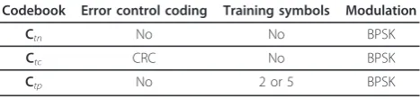
An M = 16 level uniform quantizer is considered, where each quantized value can be represented by aK= 4 bit binary sequence. We do not consider the binary quantizer, which only performs well in low observation SNR.
The codebooks used in the simulations are summar-ized in Table 1. Considering the general features of WSNs, that is, usually short data packets are transmitted and each sensor is of low cost, we use a simple error control coding (ECC) scheme, the cyclic redundancy check (CRC) codes with generation polynomial G(x) = x4 +x + 1, as an example of the coded transmission. The codebook is denoted as Ctc. For comparison,
uncoded transmission is also evaluated, where natural binary code is applied to represent each quantization, which codebook is denoted as Ctn. We consider BPSK
modulation for all codebooks. Because the code length of the uncoded transmission is shorter than that of the coded transmission, the energy to transmit each symbol will be higher for a givenEd. Due to the phase ambiguity
problem discussed in Section 5.3, we also consider the codebook with training symbolsCtp.
When CSI is known at the FC, we evaluate the perfor-mance of the MLE with codebook Ctn. The simulation
results are marked as “MLE CSI” in the legend. When CSI is unknown and the codebook is still Ctn, the
legends for MLE and the supoptimal estimator are “MLE NoCSI”and“Subopt NoCSI,” respectively. When
CSI is unknown and the codebook is Ctp, where 2 or 5
training symbols are inserted, the simulation results are marked as “MLE NoCSI TS2/5” and “Subopt NoCSI TS2/5.” We also evaluate the performance of the MLE with a near-optimal codebook obtained in [31], which is marked as “MLE NoCSI OPT.” As discussed in Section 3.2, the FC can use the training symbols to estimate the CSI and use the estimated CSI as the known CSI to esti-mate θ. We evaluate this estimator with the codebook Ctp, which is marked as“MLE EstCH TS2/5.”
To demonstrate the performance gain of the proposed estimators, two traditional fusion-based estimators and AF transmission are simulated. In the fusion-based esti-mators, the FC first demodulates the transmitted data from each sensor, then reconstructs the observation of each sensor from the demodulated symbols following the rule of quantization and finally combines these esti-mated observations with BLUE fusion rule to produce the estimate of θ. When ECCs are applied at the sen-sors, the receiver at the FC will exploit its error detec-tion ability to discard the data that cannot pass the error check. The fusion-based estimators using code-book Ctn andCtc are denoted as“Fusion-NoECC” and
“Fusion-CRC” in the legends of the figures, respectively. For AF, the amplification gainG is designed to make the average transmission power of the sensors equals to that of the digital communication schemes. We also use the MLE at the FC to estimate θ, which is marked as “AF” in the legend.
The MSE of the Quasi-BLUE [14] is shown as the per-formance lower bound with legend “Q-BLUE Bound.” This MSE is obtained in perfect communication scenar-ios with the sameM-level quantizer as other estimators.
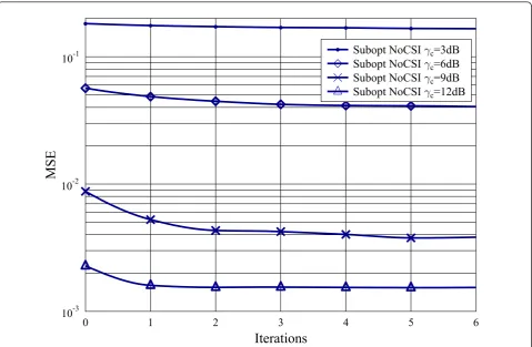
6.1 Convergence of the suboptimal estimator
We first study the convergence of the suboptimal mator. Figure 1 depicts the MSEs of the suboptimal esti-mator as a function of the number of iterations. As discussed in 5.4, at high communication SNR levels, the MSE of the suboptimal estimator is convergent after one iteration, that is, the MSE does not decrease with the iterations any more. At low communication SNR levels, the convergent speed becomes lower.
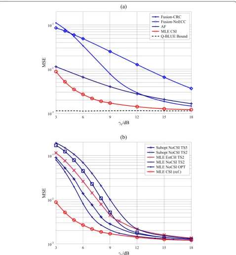
6.2 MSE versus the communication SNR
Figure 2 depicts the MSEs of the estimators with known and unknown CSI.
When CSI is known at the FC, it is shown from Fig-ure 2a that the MLE outperforms the fusion-based estimators. The MSE of the MLE approaches to the Quasi-BLUE lower bound rapidly with the increasing of the communication SNR. As expected, the MLE with AF transmission, marked as AF, is inferior to the MLE with digital communication using 4-bits
Table 1 The summary of the codebooks considered
Codebook Error control coding Training symbols Modulation
Ctn No No BPSK
Ctc CRC No BPSK
quantization, marked as MLE CSI. This justifies the conclusions in [19-21], which show that AF is not optimal in fading channels.
According to the performance analysis for BPSK mod-ulation in Rayleigh fading channels [32], the BER of the transmission scheme with codebook Ctn exceeds 0.15
whengs<3 dB. ECC can improve the transmission
per-formance for high communication SNR, but it causes more errors for low SNR. For the transmission schemes using CRC, the BER is even worse because long codes will reduce the transmission energy per symbol. For such a high BER, the fusion-based estimators do not perform well. Most of the demodulated data will be dropped due to the error check; thus, the fusion-based estimators do not have enough information to exploit, which finally leads to the worse MSE performance.
When CSI is unknown at the FC, the MSEs of the MLE with unknown CSI and with two different ways of using training symbols for channel estimation are shown in Figure 2b. One is the MLE obtained from the log-likelihood function in (42), and the other is the estima-tor obtained from (45), which uses the estimated chan-nel coefficients as their true values. As expected, our
MLE shown in (42) performs better, because it takes into account the uncertainty of the channel estimation.
Because there exists phase ambiguity in the schemes withCtn and AF transmission, simulation results show
that the MSEs of the MLE and suboptimal estimator using these two transmission schemes are very large and do not decrease when gc increases. Therefore, they are
not shown on the figures.
When we insert training symbols, the performance of the MLE with unknown CSI improves significantly, but it is still much worse than that of the MLE with known CSI at low communication SNR levels. It is interesting to see that using more training symbols does not improve the performance of the MLE as expected, because inserting training symbols will reduce the energy for the data symbols when the energy for trans-mitting an observation is fixed. Our simulations show that the best performance is obtained whenLp= 2. This
is consistent with the observation of [33], where the optimalLpequals to
√
K.
As discussed, inserting training symbols is a heuristic way to improve the performance. It is shown in the fig-ure that a codebook designed by using optimization
10-3
10-2
10-1
MSE
0 1 2 3 4 5 6
Iterations
.
.
.
.
.
.
.
Subopt NoCSI c=3dBSubopt NoCSI c=6dB
Subopt NoCSI c=9dB
Subopt NoCSI c=12dB
Figure 1The convergence of the suboptimal estimator whengs= 20 dB andN= 10. The communication SNRs are, respectively, 3, 6, 9
method outperforms all the codebooks with training symbols.
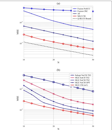
6.3 MSE versus the number of sensors
Figure 3 shows the MSEs of the estimators with known CSI and unknown CSI as a function of the number of sensorsN. We see that the MSEs of all the estimators
decrease at the speed of 1/N for large enoughN, but the MSEs do not approach the lower bound due to the communication errors. This validates our asymptotic performance analysis for the MLEs both with known CSI and with unknown CSI in 5.1. Moreover, we observe that the proposed estimators perform much bet-ter than the fusion-based estimators. It means that the
networks with conventional approaches must activate more sensors to achieve the same MSE performance as those with our estimators, which will lead to low energy and bandwidth efficiency.
7 Conclusion
In this paper, we studied decentralized estimation for a deterministic parameter using digital communications over orthogonal multiple-access fading channels with a