The Contribution of Employment Vulnerability in Explaining Private Sector Inequality in Cameroon

THE CONTRIBUTION OF EMPLOYMENT VULNERABILITY IN EXPLAINING PRIVATE SECTOR INEQUALITY IN CAMEROON

Dickson Thomas

NDAMSA1+

Gladys NJANG 2

Francis Menjo BAYE 3

1_{Faculty of Economics and Management University of Bamenda, Cameroon} 2_{Higher Teachers Training College University of Bamenda, Cameroon} 3_{Faculty of Economics and Management University of Yaoundé II,} Cameroon

(+ Corresponding author)

ABSTRACT

Article History Received: 15 February 2017 Revised: 27 April 2017 Accepted: 30 May 2017 Published: 21 July 2017

Keywords Employment vulnerability Income inequality Private sector

Within- and between-sector components

Gini coefficient Cameroon.

This paper identified the role of employment vulnerability and other regressed-income sources in accounting for private sector inequality and examined how much inequality in income and vulnerability is accounted for by within- and between-employment sector components in Cameroon. The paper employed two decomposition approaches: a regression-based framework and a Shapley Value-based rule. To attain these objectives, use was made of the 2007 Cameroon household consumption survey conducted by the government‟s statistics office. Employment vulnerability accounted for about 4.1 percent to the national private sector income inequality of 0.38, meanwhile, labour market experience, years of schooling, infant dependency and urban residency accounted for about 6.4, 10.3, 7.0 and 14.2 percent, respectively. Results also showed that the within-group components overly accounted for the national private sector income Gini inequality. Whereas, over 87 percentage points of the within-sector inequality component of 92.5 percent was accounted for by the informal sector, inequality between the formal and informal sectors of employment was only 7.5 percent. These findings highlighted the heterogeneity of informal sector activities and the wisdom of designing policies that can entice transition from informality to formal sector activities.

Contribution/ Originality: This study is first of its kind to consider the contributions of labour market factors such as longevity, employment vulnerability in examining income inequality in Cameroon. This study uses new regression-based methodology to explain income inequality. Its primary contribution is empirical knowledge on the relationship between employment vulnerability and inequality.

1. INTRODUCTION

The economic reform policies in the 1980s and the 1990s under the famous Washington Consensus1 _have recently led to growing concerns for earnings inequality. In many developing countries today, employment has become more private, especially informal; earnings shares have dropped and the gap between household earnings

1 _{The Washington Consensus in the 1980s relegated discussions on inequality to the sidelines; it regarded measures to reduce inequality as detrimental to growth,}

especially during periods of adjustment when all emphasis should be placed on reviving growth quickly. Asian Journal of Economic Modelling

ISSN(e): 2312-3656 ISSN(p): 2313-2884

DOI: 10.18488/journal.8.2017.53.274.296 Vol. 5, No. 3, 274-296

and that between employment sectors (for instances farm/nonfarm, formal/informal) have increased. These developments are controversial to some of the typical labour market elements of reform policies under the Washington Consensus such as reduction of employment protection, reduction of minimum wages, and breaking up of bargaining power. These developments may also reflect a lack of equity, social protection and social justice among labour force participants; provoking earnings disparities and job risks differential among them, especially in the private sector. The National Institute of Statistics (2011) underscored that if growth, though strong and sustainable, does not generate decent jobs (or less vulnerable jobs), it would induce wage inequalities. So taking a step to enlighten the authorities concerned with the Growth and Employment Strategy Paper (GESP) on the role of vulnerable employment on earnings inequality is vital.According to Van der Hoeven (2000) the dynamic, equity and social cohesion elements of labour market policies are important elements of redistributive and growth policies. This way, including these elements of labour market policies (for instance dynamic efficiency: increasing the quality of the labour force; and maintaining a sense of equity and social justice: reducing vulnerability among labour force participants) are necessary to reduce inequality. However, given that in the labour market we have vulnerable and decent households or groups, changes in labour market policies may have, at the very least, different consequences for particular households or groups.

In examining inequality trends in Cameroon, one observes at the national level that the Gini coefficient of total household expenditures per adult equivalent dropped fairly from 42.2% in 1984 to 40.2% in 1996. Between 1996 and 2001, inequality rose – this period corresponds to a probable consequence-period of reform policies,2 _though their responsibility may only be part of the whole. The IMF (2003) accuses inappropriate policy response to massive domestic and external debts to be part of the problem. Some argue that, because reform policies have been adopted in all developing countries and considering that most have been carried out for a decade or more, there exists a causal link between these policies and inequality trends (Van der Hoeven, 2000). Inequality in Cameroon, marginally decreased from 40.4% in 2001 to 39.0% in 2007 (Fambon and Tamba, 2010). One attractive characteristic of income inequality in Cameroon is its spatial disparity across employment sectors. For instance, private sector income inequality remains slightly higher than public sector inequality. Inequality in per capita income among private sector household heads stands at 38% compared to 37.3% in the public sector (Government of Cameroon, 2007).

Formal private sector income inequality remained higher than informal sector inequality in 2007. Per capita income inequality among formal private sector household heads stood at 38.7% compared to 35.3% in the informal sector. The same scenario is observed for farm and nonfarm private employment sectors, where nonfarm sector inequality stood at 34.3% in 2007 as opposed to 30.4% in the farming sector (GoC, 2007). This disproportionate level of inequality in farm and nonfarm as well as informal and formal private sectors may be likened to increased unemployment in nonfarm and formal sectors as well as to the growing number of low earners in these sectors. Most attempts to account for income inequality in Cameroon have either addressed accusations at sub-groups (Chameni, 2005; Baye, 2008; Essama-Nssah, 2010) or at income/expenditure components (Chameni, 2008; Miamo and Nembua, 2009; Tabi, 2009) or at individual, household and demographic characteristics (Epo et al., 2010). The contributions of labour market factors such as potential labour market experience, seniority in the main job, employment vulnerability are yet still to be considered in examining income inequality in Cameroon. In this perspective, our work attempts to provide answers to the following main research question: What are the proximate sources of earnings disparities in the Cameroon private sector?

Using the regression results displayed in the appendix, the main question can be decomposed into the following specific questions:

2 _{Episodes of Structural Adjustment programmes starting with the 1988 SAP followed by the Devaluation of 1994 of the CFA franc and the Post Devaluation}

i) What is the role of employment vulnerability and other regressed-sources in accounting for private sector inequality in Cameroon?

ii) How much inequality in a regressed-earnings source is accounted for by within- and between-components of inequality in Cameroon?

The main objective of this paper is to investigate the role of employment vulnerability among the determinants of private sector earnings inequality in Cameroon. The specific objectives are:

i) To ascertain the role of employment vulnerability and other regressed-income sources in accounting

for private sector inequality in Cameroon;

ii) To decompose income and regressed-earnings source inequality into the within- and between-components of inequality in Cameroon; and

iii) To guide ongoing and future policy on the basis of our findings and recommendations.

These objectives will inform stakeholders involved with the current Growth and Employment Strategy Paper (GESP) of the potential ills that employment vulnerability can place on the Cameroon economy in terms of widening income gaps between households involved in private employment. They will undoubtedly serve as inputs into the ongoing struggles of the Cameroon government to promote decent employment (that is, reduce vulnerable employment) and growth as a well thought package to reduce poverty.

2. LITERATURE REVIEW

Decomposition of income inequality may shed light on both its structure and dynamics. Inequality decomposition examines the contribution to inequality of particular characteristics and is important to assess the role of each characteristic to overall inequality. Inequality decomposition analyses were pioneered by Bourguignon (1979); Cowell (1980) and Shorrocks (1982;1984). Literature review on income inequality decomposition permits us to briefly disentangle four main categories of inequality decomposition.

The first category decomposes income inequality into population sub-group components such as gender, age, religion, place of residence, or region. Pioneers in this category of inequality decomposition include: Bourguignon (1979); Cowell (1980) and Shorrocks (1980;1984). Essama-Nssah (2010) like Chameni (2005) has applied this approach to decompose expenditure/income inequality among Cameroonian households into three components, intra-group, net inter-group and overlapping inter-group. Equally in this category we have Baye (2008) who has used the Shapley approach to exactly decompose inequality trends into within-group and between-group components using income and non-income well-being indicators in Cameroon.

The second category of inequality decomposition examines the different components of income/expenditure in accounting for an observed level of income/expenditure inequality. Here the level of total income/expenditure inequality is determined and thereafter decomposed into the different components of income/expenditure. Pioneers in this category include for example, Pyatt et al. (1980); Shorrocks (1982;1999) and Chantreuil and Trannoy (1999). Miamo and Nembua (2009) have used the Shapley-Shorrocks source decomposition to disentangle total income/expenditure inequality in terms of income/expenditure sources. The main income/expenditure sources used in this study include: food, housing, health, and transport expenditures.

To fill this gap, Fields and Yoo (2000) and Morduch and Sicular (2002) in the fourth category introduced a new integrated regression-based approach for decomposing income inequality indices. Their approach is an extension of the decomposition technique proposed by Shorrocks (1982;1984;1999). This approach uses estimated income flows from variables in an income generating equation (transformation of income limited at semi-log specification or the standard linear income equation) to decompose a measure of total income inequality. This method provides a rich opportunity to assess the importance of regressed variables like education, potential labour market experience, employment vulnerability and its square in explaining total inequality. Alayande (2003) has used the regression-based decomposition approach developed by Morduch and Sicular (2002) to decompose income inequality and poverty in Nigeria.

Fields (2002) attribute the variance and log-variance of the dependent variable, as a measure of inequality, to the explanatory factors and allow R2 _{to be the fraction of the variance that is explained by all the X‟s taken} together. The regression-based decomposition here is presented in the form of percentage-weights so that each factor‟s contribution is expressed as a percentage of R2_{. Besides the problems with the log-variance (see, Sen (1973)} and Foster and Ok (1999)) the decomposition of the R2 _{is heavily criticised on the basis that; R}2 _{is the fraction of} earnings/income that is explained by all explanatory variables and not necessarily the fraction of inequality explained by these variables. These problems are resolved by applying the regression-based approach combined with the natural rule of decomposition by Shorrocks (1999) or the before-after approach recommended byCancain and Reed (1998) to allow the contributions of the independent variables to sum up to total inequality (see Wan (2004) and Epo et al. (2010)).

The regression-based decomposition as introduced by Fields and Yoo (2000) and Morduch and Sicular (2002) though important, ignores the contribution of the constant and the residual terms and lays restrictions on the transformation of the dependent variable (see Wan (2002)). Wan (2002) then updates this decomposition to consider the role of the constant and the residual in explaining income inequality using this approach; which according to him constitutes vital information in the decomposition approach.

The Sub-Sahara Africa works on the regression-based decomposition approach are still somewhat fragmented. Alayande (2003) and Oyekale et al. (2006) have applied this approach in Nigeria and Epo et al. (2010) has applied the updated approach by Wan (2004) in Cameroon to decompose changes in income inequality within and between male- and female-headed households. According to Wan (2004) and Epo et al. (2010) ignoring the constant and the residual term in the regression-based decomposition is keeping aside relevant information which can help to track the unobserved determinants of income or income distribution. The recent work by Epo et al. (2010) though extend this approach to account for the marginal contributions of each independent variable including the constant and the residual term to overall inequality, does not still provide knowledge on some labour market issues in explaining income inequality across employment sectors.

Up to this stage, it is evident that works on the regression-based approach that use the natural rule of decomposition by Shorrocks (1999) or the before-after approach recommended by Cancain and Reed (1998) are still rare. The only attempts in this direction, as of now, are the works of Wan (2002) and Epo et al. (2010). Another worry is that this architecture is yet still to be employed to examine the contribution of some labour market issues in explaining income inequality across employment sectors. In this sense, our proposed study examines the contribution of variables such as education, potential labour market experience and its square, seniority in the main job, and employment vulnerability in explaining income inequality within and between households involved in farm and non-farm3_{, and between formal(private) and informal employment sectors in Cameroon.}

3. METHODOLOGY OF STUDY

In an effort to provide answers to the relevant policy question of how much inequality is accounted for by each explanatory variable, we employ a regression-based procedure (see (Fields and Yoo, 2000; Fields, 2002; Morduch and Sicular, 2002; Alayande, 2003; Fields, 2004; Wan, 2004; Epo et al., 2010)). This approach assigns weights to the explanatory variables in our earnings equation to account for earnings inequality. This approach engineers its decomposition in a way that the variation of earnings, gauged for example by an inequality measure, is broken down into the various explanatory factors such that the whole is equal to 100%4_{. We thereafter employ the approach} developed in Araar (2006a) and Baye (2008) to account for the within- and between-group inequalities of regressed-earnings sources.

3.1. Regression-Based Decomposition Approach

The literature proposes several measures to characterise inequality in the distribution of living standards (see, (Sen, 1973; Theil, 1979; Fields, 1980; Kakwani, 1980; Shorrocks, 1984; Glewwe, 1986; Litchfield, 1999)). For these authors, any good measure of inequality must satisfy at least five axiomatic conditions: (1) mean independence; (2) population size independence; (3) symmetry; (4) Pigou-Dalton transfer sensitiviy; and (5) decomposability. The inequality measures that satisfy all this criteria are the general entropy class, GE0(x), and the Atkinson measure (see, Cowell and Kuga (1981) and Shorrocks (1984)). Added to the above measures is the Gini index that satisfies all the basic axioms of an appropriate measure of inequality except the decomposability axiom. However, as indicated in Litchfield (1999) there are ways of decomposing the Gini by group but the component terms of inequality are not always intuitively or mathematically appealing. Good enough, the regression-based approach provides results across the different measures of income inequality.

Morduch and Sicular (2002) introduced a new integrated regression-based approach extending the

decomposition technique proposed by Shorrocks (1982). By letting

I

 

y

to be the weighted sum of total household

income, corresponding to a measure of inequality; a_i

 

y the proportional share of an individual or household to

total income, y; and yi the income of household i, Shorrocks (1982) developed an inequality measure expressed as a weighted sum of income:

 



_

 

i

i i

y

y

a

y

I

(1)

But since household income is observed as the sum of income from M sources or endowments,

_

  M m m i i y y 1 , the

above inequality measure can be expressed in terms of the sum-specific component, m

s

, as follows:

 

_

 

_

_

_

 

_

           m M m m i m i i i M m m i

i y y a y y s

a y I 1 1 (2)

This way, the proportional contribution of income source m,

s

m, is given by:

 

 

y I y y a s m i i i

m _



(3)

4 _{The term “decomposition” is used here in a less restrictive sense. Many studies including the literature on inequality decomposition by factor components (example}

Pyatt, Chen and Fei (1980); Shorrocks (1982); Chameni (2005); Baye (2008) and the literature decomposing differences in means between groups Blinder (1973);

According to Shorrocks (1982) the arbitrariness in the choice of the weights a_i

 

y will yield an infinite

number of potential decomposition rules for each inequality index. Thus, the value we attribute to the proportional contribution allocated to any income source can be made to take any value between minus and plus infinity. Shorrocks (1982) then goes further to increase restrictions on the choice of weights in order to derive a unique decomposition rule. These restrictions are: (1) if inequality increases or decreases by a constant amount across all income sources, the overall or total inequality is zero; and (2) if total income is divided into two components whose factor distributions are permutations of each other, their contributions to total inequality are equal. By imposing these restrictions, he obtained the unique decomposition rule below:





 

y

y

y

s

m m

var

,

cov



(4)

Morduch and Sicular (2002) extended the decomposition rule (3) to a regression-based decomposition to obtain the share of inequality attributable to the estimated income source flow of each explanatory variable. Using an

income generating function,

y



X







(where X is a vector of explanatory variables with the first column, an

n-vector of 1s, for the constant term



_o 



1,1,1,...1



;



is a vector of parameters and



is a vector of error

terms), Morduch and Sicular (2002) expressed income as a sum of predicted income and predicted error terms:





ˆ



ˆ



X

y

(5)

Equation (5) is considered as the estimated income source flow of the various household explanatory variables. The regression results allow us to make use of decomposition by income source (or factor income) since they yield estimates of income flow attributed to household variables. From the regression results, the estimated income

flows contributed by the various explanatory variables are gotten from m m

X

y

ˆ





ˆ

. It then follows that total

income is the sum of these income flows (plus the regression error term):

























ˆ

for

m

M

1

1...M

m

for

ˆ

ˆ

where

ˆ

1 1 _i m i m m i M m m i i

x

y

y

y





(6)

The share of inequality attributable to the estimated income source flow of the explanatory variable,

y

ˆ

im, is

obtained by substituting equation (6) into equation (3):

 

 

y

I

x

y

a

s

i m i i m

m







ˆ

(7)5

5 _{Morduch and Sicular (2002) suggested a simple and straight forward procedure for deriving the standard errors of}

s

m_{, but this straight forward procedure has}

been criticised by Yuko, Kim and Kimhi (2006). As with the Gini index, it is not straight forward to compute the standard errors of

s

m(see Mordarres and Joseph

Where



ˆ

m is a vector of estimated coefficients,

m i

x

the income source m attributable to household i, a_i

 

y and

 

y

I

as defined in (3).

The decomposition in equation (7) ignores the contribution of the constant term and the residual term. Wan (2004) then updates this decomposition to consider the contributions of the constant term and the residual term in explaining income inequality.

Our study uses the updated regression-based approach by Wan (2002;2004) and extends it to control for the marginal contributions of regressed earnings sources including the constant and the residual in explaining income inequality. This approach has four main advantages: (1) the approach holds other things equal; (2) decomposition is done in a way that the contributions of the several independent variables sum to the contributions of the overall model; (3) it allows for variations in the dependent variable to be gauged by an index other than the variance; and (4) Wan (2002) shows that this approach allows for identification as well as quantification of roots or determinants of inequality. The number of exogenous variables can be arbitrary with proxies being used as need arises.

Our earnings equation can be rewritten to take the following form:

i m i m i

i

i

x

x

x

Y





₀





₁ 1





₂ 2

















(8)

Where, Yi is the log of household per capita earnings,



is the vector of parameters, X is the vector of

independent variables and



is the error term. The independent variables, X, include: education, potential labour market experience and its square, employment vulnerability6_{, marital status, control for gender-dummy, location} and for socio-professional status in the main job.

In order to purge restrictions on the transformations of the dependent variable and pitfalls related to the constant and the residual term, let‟s express our estimated earnings function as follows (see, Wan (2002;2004)):

 











 







F

X

Y

X

Y

₀ * (9)

Where, Y is the earnings function (per capita earnings) or its transformation such as the logarithm of earnings

(LnY), X is a vector of income determinants,



₀ is the constant term,



is the error term and Y*(X) is the

estimated income source. F(X) allows for any form (linear with the presence of the constant term or highly non-linear with the absence of this term) and other transformations of income (original income or logarithm of income) can be used as the dependent variable.

Let









i

m

m

X

Y

X

Y

*

(

)



where,

Y

i





m

X

m represents the income flow from the mth factor.

Let

Y

ˆ

denotes the determinist part of equation (9). Basing on equations (9) and (8) we can have:













i i

Y

Y

Y

Y

0

*

0

ˆ

ˆ

_

_

_{. We can rewrite equation (9) as:}







Y

Y

ˆ

(10)

To account for the contribution of



, we follow Shorrocks (1999) by removing



from equation (10) and obtain:



Y



I

 

Y

I

/





0



ˆ

Where

I

 



represents an inequality measure.

We can then determine the contribution of the residual term to inequality, I(Y), as follows:

 

Y

I

 

Y

I

S







ˆ

(11)

The decomposition makes intuitive as well as theoretical sense, since the ranking of

Y

and

Y

ˆ

differs and would

be equivalent only if there is good enough fit of the earnings function.

Now focusing on the constant term, we can write 0

*

ˆ

_

_Y

_

_

Y

. Applying the natural rule of Shorrocks (1999) we

have:





 

*

0

0

/

ˆ

_I

_Y

Y

I







This way, the contribution made by the constant term is simply:

 

 

*

0

ˆ

Y

I

Y

I

S





(12)

Lastly, the contribution of the estimated income factors is straightforward:

 

*

Y I

Sm  (13)

Therefore inequality, I(Y), can be decomposed into

S

,

S

0, and

S

m which represent the contributions made

by the residual term, the constant term, and the estimated factor sources respectively. These contributions can be expressed in percentages summing to 100%.

This paper uses this architecture to examine the contribution of some labour market variables in explaining income inequality among private sector household heads in Cameroon. Knowledge on the contribution of variables such as education, potential labour market experience and its square, seniority in the main job, employment vulnerability in explaining income inequality among private sector workers as well as the within- and between-group components that account for income inequality across employment sectors (farm and non-farm as well as across formal and informal) in Cameroon is vital for policy action. Moreover, the consideration of the constant term which can be liken to a headcount tax (negative constant income) or a headcount subsidy (positive constant income) permits policy analysts to understand the role of a headcount tax or headcount subsidy in increasing or decreasing inequality in Cameroon respectively.

In summary, it is straightforward that measured inequality, I(Y), is decomposed exactly into the contributions of the various explanatory variables X‟s, the constant term and the residual term. The regression based-decomposition framework used is independent of the inequality measure used. Equally, any arbitrary transformation of the target variable is allowed, as inequality would be measured on the transformed value (see, (Fields and Yoo, 2000; Epo et al., 2010)). Moreover, even if the dependent variable is transformed, inequality may still be measured over the original variable by this procedure.

3.2. Sectoral Inequality Decomposition of Regressed-Earnings Sources

inequality of income and the regressed-earnings source vulnerability are decomposed into within- and between-group inequalities across (for example, employment sectors; farm/nonfarm and formal/informal).

Sub-group Decomposition of the Gini: The Shapley Value Approach7

The Shapley Value decomposition rule is designed to obtain exact decomposition of the Gini coefficient into within- and between-group components that purge the overlapping term (Araar, 2006a; Baye, 2008). The application of this approach is two-fold. The first fold consist in decomposing the overall Gini index per regressed source of earnings into and between-group contributions. The second phase entails the expression within-group contribution as a weighted sum of the within-within-group contribution by the different employment sectors. Let

)

~

(

Y

G

be the total Gini index per regressed source of earnings, then we can express:

G

(

Y

~

)



v



W

_g

,

B

_g



(14)

Where Wg and Bg are the within- and between-group inequalities and v is a characteristic function.

In the first phase, we suppose that the within-group inequality component

 

G

_Wsh and the between-group inequality

component

 

sh B

G exactly account for the overall Gini coefficient per regressed source (

G

 

Y

~

). To compute the

marginal contributions of each of these factors, the basic rules to follow are: (1) eliminate the between-group inequality and compute the within-group inequality by using a vector of a regressed source of earnings where each

household‟s endowment has been multiplied by





K . This operation renders the average endowment of each

group to equal



; (2) eliminate the within-group inequality and compute the between-group inequality,



K



G



₁

,...,



by using a vector of regressed endowment where each household has the average endowment of

its group, denoted



K; and (3) eliminate between- and within-group inequality simultaneously and each household

is left with the average regressed endowment. In this case,

G

(



)



0

.

The above elimination order is arbitrary and the arbitrariness is removed by obtaining the Shapley Value within- and between-group contributions as follows:







 

 



     ( ) ( ) ( ) 2 1 0 , 2 1   

 G Y G

G v G W v B v B W v G K K g g g g sh W       

 ₍₁₅₎

and







 

 



     ( ) ( ) ( ) 2 1 0 , 2 1   

 G G

Y G v G B v W v B W v G K K g g g g sh B       

 (16)

From the within-group contribution to overall inequality expressed in equation (15), the second step consists of

decomposing global within-group inequality as a sum of within-group inequality across groups. With

G

(



)



0

,

the within-group contribution is then based on three inequality indices. The same rule is used for determining the

impact of eliminating the marginal contribution of group k, notably the attribution of group k‟s average share to all its members in order to eliminate the group‟s contribution to global within-group inequality. This gives us the Shaply Value of group k‟s contribution to total within-group inequality.

To illustrate this procedure, let‟s use two groups A and B (for example, A= farm sector of employment and B = nonfarm or A = informal and B = formal private), equation (5.15) is restated as follows:



















A B A A B B



sh

W

G

Y

G

G

Y

i

Y

i

G

(

)



,



,





,

,





2

1

_

_



(17)

The Shapley Value contribution of group A to global within-group inequality is given by:









































































           





            , , , , , , , , , , , , , , , ) ( 4 1 G i Y G i Y G i Y i Y G G G G G G Y G Y G Y G G A A B B B B A A B A B A B A B A B A B A B A sh W             (18) The same procedure can be done symmetrically for the second group.

4. DATA USED AND JUSTIFICATION OF INEQUALITY MEASURES USED 4.1. Data Presentation

Use is made of the estimated variables in the regression table in the appendix (Appendix B), generated from CHCS III conducted in 2007 by the National Institute of Statistics (NIS). The CHCS III survey was conducted between May and July 2007; and comprised 11391 households that were actually interviewed. This data set divides the country into 22 strata: Douala; Yaoundé; and 10 semi-urban and 10 rural areas.

Table-1. Indicator variables/modalities

Variables Variables

Employment contract Piece rate

Open-ended (written) Commissions/benefits

Fixed term (written) Inkind /no payment

Verbal agreement Labour status

No contract Permanent regular

Payslip Permanent seasonal

Yes Indifferent8

No Temporary undefined/ defined

Social security

Yes Family allowance

No Yes

Job satisfaction No

Yes Housing allowance

No Yes

Underemployment No

Less hours fixed by employer Paid leaves

Indifferent Yes

Less hours due to economic situation No

Less hours due to health problems and domestic work Union membership

Remuneration Yes

Fixed salary No

Daily/hourly pay

Indifferent

Source: constructed by author

8 _{The sub-category “indifferent” captures all those household heads who did not provide an answer (missing) and/or those who answered “don‟t know” or nsp (ne sait}

Out of this total of 11391 households interviewed, 9219 are actively employed in private sector activities, 1102 are involved in the public, para-public and international organisations, and the remaining 1070 are unemployed, discouraged unemployed and inactive. This data set provides a number of employment status indicators for the household head‟s (main and second job), which better add up the multifaceted nature of employment vulnerability in the main job. Table 1 summarises the initial indicators used to build the employment vulnerability index.

The dependent variable for our study is per capita monthly earnings. Exogenous included variables are employment vulnerability (index), education (years); experience (years of work) and its square; seniority in the main job (dummy); number of younger children (cluster level); Number of married household heads (cluster level), gender (dummy); and location (dummy). Other variables: sector of employment (farm/nonfarm, and formal/informal).

4.2. Description of Inequality Indexes Used

There are many inequality measures in the literature; Coulter (1989) even identified about 50 (fifty) different inequality measures. But Litchfield (1999) posited that only a few have the “desirable properties” required to be a good inequality measure9_{. Though, apparently, there seem to be no consensus on how best to measure inequality} (Olaniyan and Awoyemi, 2005). Debate on the merits and demerits of various desirable properties is almost giving way to a consensus on this subject (Morduch and Sicular, 2002; Oyekale et al., 2006). Cavendish (1999) broadly classified inequality measures into normative and positive measures, where the positive measures are indices that summarise features of statistical dispersion in income distribution and normative measures are derived by imposing restrictions on the inequality function derived from well stated ethical beliefs underlying the societies‟ concern for inequality (Olaniyan and Awoyemi, 2005). For instance, positive measures include the Gini coefficient, the coefficient of variation, the relative mean deviation and the variance of logarithms.

The Gini index developed by Gini in 1912 is a widely used measure of inequality because it satisfies all the basic characteristics of a good measure except the decomposability criteria if the sub-sectors of income overlap. However, many authors have shown that Gini coefficient can be decomposed successfully (Litchfield, 1999). Araar (2006a) has even pointed out that the Gini coefficient is the most suitable for source decomposition. The Gini coefficient measures the ratio of the area between the Lorenz Curve and the iso-distribution line to the area of maximum concentration. The Generalised Entropy class (

) and the Atkinson measure meet all the basic criteria of a good inequality measure (Cowell and Kuga, 1981; Shorrocks, 1984). However, it is necessary to highlight that these two measures are not significantly different as the Atkinson index is simply the transform of the

measures. Thus, both the

and the Atkinson indexes rank income identically (Cowell and Kuga, 1981). The

class have some attractive characteristics as they are sensitive to changes at the lower end of the distribution for close to zero. GE(0) is identical to mean log deviation. Equally, they are sensitive to changes across the distribution for equal to one (which is the Theil index), and sensitive to changes at the higher end of the distribution for higher values (for instance =2)10_{. GE(2) is half the squared coefficient of variation (which is} the Generalised Entropy index) (Cavendish, 1999). When

equals zero, there is perfect equality in the distribution. The

class is fundamentally useful in sub-group decomposition analysis but not suitable for source decomposition analysis.

The coefficient of variation (CV) meets some of the properties for a good measure of inequality except the uniform addition and decomposability criteria. The CV measures inequality as the standard deviation of a distribution divided by its mean. It measures the degree of concentration and is related to the second-order stochastic dominance. This measure has been employed in most regression-based decomposition analysis including Morduch and Sicular (2002); Wan (2002) and Epo (2012). In the nutshell, the coefficient of variation squared

9 _{(1) Mean independence; (2) population size independence; (3) symmetry; (4) Pigou-Dalton transfer sensitiviy; (5) decomposability; and (6) Statistical testability..}

measures inequality as the variance of a distribution divided by the square of its mean. This measure is particularly important when it comes to studying the degree of dispersion or concentration.

5. EMPIRICAL RESULTS

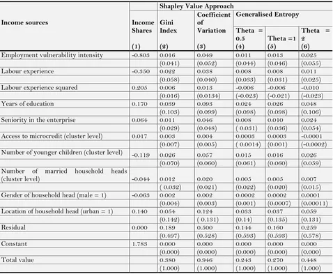
Table 2 hosts the income shares of predicted earnings sources to total household per capita earnings. This table shows the substantial share made by human capital variables in determining total household per capita earnings. Cumulated labour market experience (experience squared) and years of schooling jointly accounted almost 38% of private sector earnings, with labour experience squared registering the highest earnings share. Urban residency and holding a managerial position in the enterprise also have considerable earnings shares. This is probable as majority of urban dwellers have access to well-paid jobs compared to their rural counterparts. Another estimated source that may complement total household earnings, though marginally, is access to microcredit at the cluster level.

Our results indicate that employment vulnerability registered the largest diluting share on total household per capita earnings of private sector workers. This is indication that in the private sector, the net effect of employment vulnerability is lower household earnings. Worthy to note, the number of young children in a household also dilute total household per capita earnings considerably.

Table-2. Total earnings Inequality Decomposition by estimated earnings sources

Income sources

Shapley Value Approach

Income Shares

(1)

Gini Index

(2)

Coefficient of

Variation

(3)

Generalised Entropy

Theta = 0.5

(4) Theta =1 (5)

Theta = 2

(6)

Employment vulnerability intensity -0.803 0.016 0.049 0.011 0.013 0.025

(0.041) (0.052) (0.044) (0.046) (0.055)

Labour experience -0.350 0.022 0.038 0.008 0.008 0.011

(0.058) (0.040) (0.033) (0.031) (0.025)

Labour experience squared 0.205 0.006 0.013 -0.006 -0.006 -0.010

(0.016) (0.0134) (-0.023) (-0.021) (-0.023)

Years of education 0.170 0.039 0.093 0.024 0.026 0.048

(0.103) (0.099) (0.098) (0.098) (0.106)

Seniority in the enterprise 0.064 0.011 0.046 0.008 0.010 0.024

(0.029) (0.048) ( 0.031) (0.036) (0.054)

Access to microcredit (cluster level) 0.017 0.003 0.004 0.0003 0.0003 -0.0001

(0.007) (0.005) ( 0.0014) (0.001) (-0.0002)

Number of younger children (cluster level) -0.119 0.026 0.057 0.015 0.016 0.026

(0.070) (0.060) (0.061) (0.060) (0.059)

Number of married household heads

(cluster level) -0.044 0.012 0.020 0.005 0.005 0.007

( 0.032) (0.021) (0.022) (0.020) (0.015)

Gender of household head (male = 1) -0.063 0.002 0.002 0.0002 0.0002 0.0001

(0.004) (0.003) (0.001) (0.0007) (0.00011)

Location of household head (urban = 1) 0.140 0.054 0.124 0.033 0.037 0.059

(0.142) ( 0.131) (0.14) (0.135) (0.131)

Residual 0.000 0.189 0.500 0.144 0.160 0.259

(0.497) (0.528) (0.593) (0.593) (0.578)

Constant 1.783 0.000 0.000 0.000 0.000 0.000

(0.000) (0.000) (0.000) (0.000) (0.000)

Total value 0.380 0.946 0.243 0.270 0.448

(1.000) (1.000) (1.000) (1.000) (1.000)

5.1. The Contributions of Estimated Earnings Sources to Measured Inequality in the Private Sector

Table 2 submits the exact contributions of the predicted earnings sources to total earnings inequality for the Gini index, Coefficient of Variation (CV), and the Generalised entropy (GE) measure (Theta 0.5; 1; and 2). Columns 2, 3, 4, 5, and 6 host the Gini, CV and GE measures (Theta = 0.5, Theta = 1, and Theta = 2) respectively. Though detailed interpretations are done with respect to the most popular and widely used Gini index, some discussions are made with regards to the GE and CV; that track the behaviour of the estimated sources at the lower and upper tails of income distribution and to study the degree of dispersion respectively.

From Table 2 employment vulnerability increases earnings inequality by more than 4% in the private sector (column 2). This cankerworm, employment vulnerability, which has the habit of diluting market earnings in developing countries, may be qualified as “a thing of the poor”. It does no less than worsening earnings inequality between the poor and the rich or between the informal and the formal sector or between rural and urban areas as intimated earlier in this study. Employment vulnerability is thus a threat that widens earnings inequality among private sector household heads. This observation ties with the NIS (2011) who posited that growth that does not generate decent jobs may induce earnings inequalities and social strife (p. 4-5). The years of schooling and labour market experience increase earnings inequality in the private sector. This result is probable, given the prevailing situation in the Cameroon private sector. To begin, most education programmes and capacity building workshops largely benefit the rich than the poor. Equally, the return to education is somewhat low in the private sector; as a household head in the private sector earns on average 24 730 CFA francs per month compared to 36 100 CFA francs for a public sector household head (GoC, 2007). This may be due to the scarcity of job opportunities in the country as a whole. This result may also be justified by the observation that, in the private sector, about 33.3% have no education and a large proportion (37.4%) have only completed primary school (GoC, 2007) which cannot secure a well paid job in the private sector.

Holding a managerial position also increases earnings inequality in the private sector, as this position that attracts higher earnings is held by very few. In Cameroon, only 8% of private sector household head hold managerial or supervisory positions. Access to microcredit tends to increase earnings inequality. This is probable as the poor household heads rarely benefit from microcredit as a result of lack of appropriate guarantee or collateral security and poor projects. This leaves the poor with lack of financing to start-up micro-activities or businesses that can generate income. This highlights that a tour back to the standard approach of microfinance11 _{may be a good} avenue for inequality squeezing. This corroborates with Oyekale et al. (2006) who found that access to formal and informal credit tends to increase income inequality (p. 24).

Male household headship unlike urban residency increase, though marginally, earnings inequality. Residing in an urban area tends to increase earnings inequality by almost 14%. This is attributable to the relative availability of well paid jobs in the urban than rural areas. Efforts to encourage the planting of industrial establishments and transformation units in rural areas may prove fertile. The number of young children below 5 (five) years old and the number of married people at the cluster level tend to increase earnings inequality. This is evident as the presence of young children reduces involvement in productive activities, in terms of hours worked. This shows that birth control and family planning should also be integrated in poverty alleviation and inequality reduction measures.

Unlike the constant with a zero contribution, the residual term registers a substantial contribution to the measured Gini index. However, its contribution (of almost 49.7%) is far below the threshold of 80% fixed by Wan (2002) for studies with limited value. This term tracks the contribution of non-included determinants of private sector earnings in Cameroon. The same interpretations and policy messages, obtain with the Gini coefficient, can be drawn with the coefficient of variation (Table 2, column 3), though with some variability in the magnitude of the contributions of earning sources.

Columns 4, 5, and 6 submit the regression-based decomposition results by predicted earnings sources, using the generalised entropy; Theta = 0.5, Theta = 1, and Theta = 2, respectively. The generalised entropy has the peculiarity of measuring inequality at a given level of income distribution. Here we consider Theta = 0.5 and 2 to track the contributions of regressed earnings sources to earnings inequality at the lower and upper tails of the distribution of living standards. This endeavour will inform policy makers on the variables-cum policies that account for earnings inequality among private sector workers at the lower and upper tails of earnings distribution, often likened to the poor and rich tails respectively. We also consider Theta = 1 which allows equal weighting across the distribution of living standards for purpose of comparison.

As theta tends to 0.5, we observe that the earnings inequality increasing effect of employment vulnerability is more pronounced among private sector household heads at the upper tail of the distribution of earnings than those at the lower tail. Employment vulnerability accounts for about 4.4% of measured earnings inequality among household heads at the lower tail of the distribution of earnings compared to 5.5% for those at the upper tail. This is evident as programmes to enhance the working conditions of household heads may by-pass the poorest of the lower tail and the poor of the upper tail and mainly benefit the better-off in these classes. This is indication that efforts to reduce the vulnerability of private sector workers at the lower and upper tails of distribution of earnings are tantamount to reducing overall private sector earnings inequality. Years of schooling and labour experience increase earnings inequality in the lower and upper tails of earnings distribution. This is due to obvious reasons; as most education enhancement programs by-pass the poorest of the lower tail and the poor of the upper tail. Years of schooling account for 9.5% of earnings inequality at the lower tail of earnings distribution compared to 9.8% in the upper tail. This shows that education programs specifically designed for the poorest of the lower tail and the poor of the upper tail can mitigate the inequality gap among private sector household heads.

Job experience square on her part reduces earnings inequality in the lower and upper tails of earnings distribution. This indicates that capacity building programmes to enhance the skills of private sector workers may mitigate to reduce inequality in income. Holding a managerial position account for almost 4.2% of earnings inequality among private sector workers at the lower tail of the distribution compared to 6.8% for those at the upper tail. This is most likely as the poorest of the lower tail and the poor of the upper tail are most unlikely to hold managerial or supervisory positions in enterprises. Access to microcredit increases inequality among lower and upper tail household heads. This is probable as the poorest household heads in the lower tail and the poor in the upper tail may lack the necessary collateral or guarantee required by lenders. This observation is relevant given the gradual passage of microfinance approach from poverty reduction to financial sustainability, where poor (or poorest) household heads are increasingly being considered risky borrowers.

The number of young children and the number of married household heads at the cluster level increase earnings inequality in the lower and upper tails of the distribution of earnings. The number of young children account for almost 5% of measured earnings inequality in the lower tail compared to 4.5% in the upper tail. This is indication that birth control and family planning programmes specifically designed for the poorest and poor household heads should be incorporated in anti-inequality strategy packages. Being male gender type and residing in the urban area increase earnings inequality as intimidated earlier.

5.2. Sectoral Decomposition of Earnings-Source Inequality With and Without Vulnerability, and Vulnerability Inequality

compared to the between-group contributions of 7.5 per cent and 26.5 per cent. The bulk of the within-sector earnings source inequality was registered in the informal and farming employment sectors (Table 3 and 4). The informal sector over accounted 87.7 percentage points of the within-sector earnings source inequality compared to about 4.8 percentage points for the formal private sector (Table 3). In the same light, the farming sector over-accounted 44.2 percentage points of the within-sector earnings source inequality among private sector workers as opposed to 29.3 percentage points for the nonfarm private sector (Table 4). This is indication that more targeted policy objectives that focused on reducing earnings source inequality among household heads involved in the informal and farming employment sectors may have considerable effects on overall private sector earnings inequality.

Table-3. Sectoral Decomposition of source inequality with and without vulnerability: Formal and informal employment sectors

Shapley Value Decomposition of the S-Gini Coefficient

Sector S-Gini Source Inequality _{with vulnerability}

S-Gini Source

Inequality without

vulnerability Change Vulnerability source S-Gini

Estimate RCi Estimate RCi Estimate RCi Estimate RCi

Informal 0.334 0.877 0.318 0.882 0.016 -0.005 0.112 0.356

Formal 0.018 0.048 0.037 0.101 -0.019 -0.053 0 .026 0.083

Intra_group 0.352 0.925 0.355 0.983 -0.003 -0.058 0.138 0.44

Inter_group 0.028 0.075 0.006 0.017 0.022 0.058 0.176 0.56

Overall Private 0.380 1.000 0.361 1.000 0.019 0.000 0.314 1.000

Source: Computed by authors from CHCS 2007 Survey data using DAD 4.5 Software for Distributive Analysis.

Note: RCi stands for relative contributions

Considering the sectoral decomposition of earnings source inequality without vulnerability, the S-Gini drops to 36.1% at the overall level (Tables 3 and 4). The within-sector component still prevails in explaining overall earnings source inequality without vulnerability in both the informal/formal and farm/nonfarm private sectors. However, we observe that inequality within the informal sector drops from 33.4% to 31.8% and the relative contribution of the informal sector to within-group inequality drops by 0.5%. This shows that employment vulnerability worsens earnings inequality among household heads involved in informal activities. For the farm/nonfarm employment sectors, employment vulnerability worsens inequality among household heads involved in farming activities with respect to those in the nonfarm private sectors.

Table-4. Sectoral decomposition of source inequality with and without vulnerability: Farm and nonfarm employment sectors

Sector

Shapley Value Decomposition of the S-Gini Coefficient

Source S-Gini

Inequality with

vulnerability Source S-Gini Inequality without vulnerability Change Vulnerability source S-Gini

Estimate RCi Estimate RCi Estimate RCi Estimate RCi

Farm 0.168 0.442 0.178 0.492 -0.010 -0.05 0.092 0.293

Nonfarm 0.112 0.293 0.135 0.373 -0.023 -0.08 0.145 0.464

Intra_group 0.28 0.735 0.312 0.865 -0.032 -0.130 0.237 0.757

Inter_group 0.101 0.265 0.049 0.135 0.052 0.130 0.076 0.243

Overall private 0.38 1.000 0.361 1.000 0.027 0.000 0.314 1.000

Source: Computed by authors from CHCS 2007 Survey data using DAD 4.5 Software for Distributive Analysis. Note: RCi stands for relative contributions

These two dimensions of well-being (Earnings source inequality - with and without vulnerability - and employment vulnerability) do attest to the dominant contribution of within-group inequality in the distribution of well-being in the Cameroon private sector. However, while the between-group contribution is negligible in the earnings source dimension – with and without vulnerability - for the formal/informal employment sectors, it is non-negligible in the vulnerability dimension of inequality (Table 3). These results indicate that better policy outcomes could be reached in reducing private sector earnings source inequality if policy objectives are aimed at tackling inequality within the formal and informal employment sectors and very little could be achieved if emphasis is placed on sectoral disparities. Concerning the vulnerability dimension in the formal/informal employment sectors, opting for an optimal-mix of within- and between-group policy orientations, with more emphasis on the between component, appears to be more appropriate in down-scaling vulnerability source inequality in formal/informal employment sectors rather than focusing only on one orientation.

For the farm/nonfarm employment sectors, the between-group contribution is non-negligible in both dimensions, but quite more considerable in the earnings source with vulnerability than in that without vulnerability (Table 4). This implies that greater efficiency could be achieved in reducing earnings source and vulnerability inequalities in the private sector if both within- and between-group considerations are targeted disproportionately in the farm/nonfarm sectors. Worthy to recall that more emphasis on within-sector earnings source and vulnerability source inequalities is likely to produce greater impacts on overall private sector earnings source and vulnerability inequalities. However, the emphasis to lay on the between-group consideration may not level-up along the earnings source and vulnerability dimensions.

6. CONCLUDING REMARKS AND POLICY IMPLICATIONS

This paper attempted to identify the role of employment vulnerability and other regressed-sources in accounting for private sector inequality and to examine how much inequality in income and vulnerability is accounted for by within- and between-employment sector components of inequality in Cameroon. Thus, the paper first employed the regression-based decomposition architecture to examine the contribution of some labour market variables in explaining income inequality among private sector household heads in Cameroon. Then we used the Shapley Value decomposition rule to obtain exact decomposition of the Gini coefficient into within- and between-group components. The regression-based decomposition provided results for the Gini index, Coefficient of Variation (CV), and the Generalised entropy (GE), though interpretations were made with respect to the most popular and widely used Gini index.

“poorer”12 _{employment sectors. Equally, years of schooling and labour market experience increased earnings} inequality in the private sector. This was likened to the prevailing situation in the Cameroon private sector, where most education programmes and capacity building workshops largely benefit the rich than the poor. This result was also justified by the observation that, in the private sector, about 33.3% have no education and a large proportion (37.4%) have only completed primary school (GoC, 2007) which cannot secure a well paid job in the private sector. Holding a managerial position and access to microcredit were also found to increase earnings inequality in the private sector. Residing in an urban area tended to increase earnings inequality by almost 16%.

In 2007, we found that of the income S-Gini of 38.1 per cent, the within-group component overly accounted 92.5 per cent and 73.5 per cent in the formal/informal and farm/nonfarm sub-sectors respectively compared to the between-group contributions of 7.5 per cent and 26.5 per cent. The bulk of the within-group income inequality was registered in the informal and farming employment sectors. In the period under review, the within-group component overwhelmingly accounted for the vulnerability S-Gini of 5.8 per cent in both the formal/informal and farm/nonfarm private employment sectors. The informal employment sector and the nonfarm private over-accounted for the within-group vulnerability inequality compared to the formal sector and farming sector.

Efforts to encourage the formalisation of the informal sector may be very fertile for policy administration and designing. More targeted policy objectives that focused on reducing vulnerability inequality among household heads involved in the informal and farming employment sectors may have considerable effects on overall private sector income inequality. Equally, policy efforts to check vulnerability inequality in these sectors are likely to generate greater impacts on overall private sector vulnerability inequality. Thus initiatives like the one-stop shop by the government of Cameroon to facilitate creation of enterprises and formalization of those in informal activities should be encouraged and perpetuated. Conventions with the ILO that can improve the working conditions of private sector household heads in Cameroon should be embraced. Importantly, the quality-employment or decent employment driven growth enshrined in the GESP by the government of Cameroon should be followed-up to ensure an objective implementation of the designed strategies. However, for the government of Cameroon to know success with the GESP, in terms of decent employment, more targeted policy measures to improve the working conditions of workers in informal and farming activities is strongly recommended. The reduction of employment vulnerability may pair-up fairly well with education/capacity building programmes as well as measures to improve credit access for those household heads in informal and farming sectors to produce very commendable effects on overall private sector income inequality.

Funding: This study received no specific financial support.

Competing Interests: The authors declare that they have no competing interests.

Contributors/Acknowledgement: All authors contributed equally to the conception and design of the study.

REFERENCES

Alayande, B., 2003. Development of inequality reconsidered: Some evidence from Nigeria. Paper Presented at the UNU-WIDER Conference on Inequality, Poverty and Human Wellbeing in Helsinki, Finland between 29th and 31st May 2003. Araar, A., 2006a. On the decomposition of the gini coefficient: An exact approach, with illustration using cameroonian data.

Cahiers de Recherché, 0602, CIRPEE.

Araar, A. and J. Duclos, 2009. Distributive analysis stata package (DASP) 2.1 Software. University of Laval, CIRPEE and the Poverty Economic and Policy Research Network.

Asselin, L.M., 2002. Composite indicator of multidimensional poverty. Centre interuniversitaire sur le Risque, les Politiques Économiques et l'Emploi, Laval University and Institut de Mathématique Gauss: Lévis, Québec.

12 _{Poorer in terms of social and institutional protection, for instance farming and informal employment sectors as compared to nonfarm and formal employment}

Baye, M.F., 2008. Exact configuration of poverty inequality and polarisation trends in the distribution of well-being in Cameroon. Paper Presented at the Centre for the Study of African Economies (CSAE), Conference 2008 on „Economic Development in Africa‟, St Catherine‟s College, Oxford.

Benzécri, J.P., 1979. Sur le calcul des taux d'inertie dans l'analyse d'un questionnaire. Les Cahiers de l'Analyse des Données, 4(3): 377-378.View at Google Scholar

Blinder, A.S., 1973. Wage discrimination: Reduced form and structural estimates. Journal of Human Resources, 8(4): 436-455.

View at Google Scholar | View at Publisher

Bourguignon, F., 1979. Decomposable income inequality measures. Econometrica, 47(4): 901-920. View at Google Scholar | View at Publisher

Cancain, M. and D. Reed, 1998. Assessing the effect of wives‟ earnings on family income inequality. Review of Economics and Statistics, 80(1): 73-79.View at Google Scholar | View at Publisher

Cavendish, W., 1999. Poverty, Inequality and environmental resources: Quantitative analysis of rural households CSAE Working Paper No. 99-9 February 1999.

Chameni, N.C., 2005. A three components subgroup decomposition of the Hirschman-herfindahl index and household income inequalities in Cameroon. Applied Economics Letters, 12(15): 941-947.View at Google Scholar | View at Publisher

Chameni, N.C., 2008. The “natural” bidimensional decomposition of inequality indices: Evaluating factors contribution to households welfare inequality in Cameroon, 1996-2001. Applied Economics Letters, 15(12): 963-970. View at Google

Scholar | View at Publisher

Chantreuil, F. and A. Trannoy, 1999. Inequality decomposition values: The trade-off between marginality and consistency. DP 99-24 THEMA.

Coulter, P.B., 1989. Measuring inequality: A methodological handbook. Boulder: Westview Press.

Cowell, F.A., 1980. On the structure of additive inequality measures. Review of Economic Studies, 47(3): 521-531.View at Google

Scholar | View at Publisher

Cowell, F.A. and K. Kuga, 1981. Additivity and the entropy concept: An axiomatic approach to inequality measurement. Journal of Economic Theory, 25(1): 131-143.View at Google Scholar | View at Publisher

Epo, B.N., 2012. Determinants of poverty, inequality and gender disparity in the distribution of household welfare in Cameroon: 2001-2007, Unpublished Ph.D Thesis, Department of Economics and Management, University of Yaoundé II.

Epo, B.N., M.F. Baye and N.A. Manga, 2010. Explaining spatial and inter-temporal sources of poverty, inequality and gender disparities in Cameroon: A regression-based Decomposition analysis. PEP Research Network, Research Paper N°11321. Retrieved from www.pep-net.org.

Essama-Nssah, 2010. A counterfactual analysis of the poverty impact of economic growth in Cameroon. World Bank Research Working Paper No. 5249. World Bank, Washington, DC.

Fambon, S. and I. Tamba, 2010. Spatial inequality in Cameroon during the 1984-2007 period. AERC Collaborative Research on Growth and Poverty Reduction, 28 November – 03 December 2010, Mombasa, Kenya.

Fields, 2002. Accounting for income inequality and its change: A new method, with application to the distribution of earnings in the United States. Research in Labour Economics.

Fields, 2004. Regression-based decompositions: A new tool for managerial decision-making. Cornell University, New York: Department of Labour Economics.

Fields, G.S., 1980. Poverty, inequality and development. Cambridge: Cambridge University Press.

Fields, G.S. and G. Yoo, 2000. Falling labour inequality in Korea‟s economic growth: Patterns and underlying causes. Review of Income and Wealth, 46(2): 139-159.View at Google Scholar | View at Publisher

Foster, J.E. and E.A. Ok, 1999. Lorenz dominance and the variance of logarithms. Econometrica, 67(4): 901-907.View at Google

Scholar | View at Publisher