Predictable Returns and Non-Synchronous Trading

(1)

Predictable Returns and Non-Synchronous Trading

Latifa Fatnassi (Research Scholar, Faculty of Economics and Management, Tunis, Tunisia)

Ezzeddine Abaoub (Aggregate Professor, Faculty of Economics and Management, Tunis, Tunisia)

(2)

238

Author(s)

Latifa Fatnassi

Research Scholar, Faculty of Economics and Management, Tunis, Tunisia

Ezzeddine Abaoub

Aggregate Professor, Faculty of Economics and Management, Tunis, Tunisia

Predictable Returns and Non-Synchronous Trading

Abstract

The aim of this paper is to investigate non-synchronous trading effect in terms of predictability. This analysis is applied to daily and one-minute interval data on the KOREA stock market. The results indicate evidence of predictability between indices with different degrees of non-synchronous trading and when considering one-minute interval data. We then propose a simple test to infer whether such predictability is mainly attributing to non-synchronous trading or an actual delayed adjustment on part of traders. The results obtained suggest that the observed predictability is attributed to non-synchronous trading instead of delay adjustments in price to the “news”.

Keywords: Return predictability, lead-lag effect, emergent market, impulse-response function, granger-causality

Introduction

Several studies have investigated the effect of non-synchronous trading on the autocorrelation of returns i.e. Lo and Mackinlay (1990), Schotman and Zalewska (2006). All the studies conclude that the non-synchronous trading increases the serial correlation of returns. Lo and Mackinlay (1990) proposed an econometric model of non-synchronous trading by analyzing its implications on returns of individual securities and portfolio. They found that ignorance of an non-synchronous trading may bias the results and generate inferences completely false: The non-synchronous trading generates a negative serial in returns of individual securities while a positive serial correlation in observed portfolio returns.

The impact of non-synchronous trading on predictability returns has been studies by Camilleri and Green (2004) on the Indian market using three approaches: Test Pesaran Timmermann, VAR model, Granger-Causality and Impulse-response function on daily and high frequency data. The results imply that non-synchronous trading appears to be the main source of the predictability of returns on the Indian stock market. More specially, the purpose of this paper is to study the impact of non-synchronous trading on the predictability

of returns of Korea stock market and examine the main cause of this effect. We propose a new alternative focuses on the study of lead-lag effect on the value of indices by adopting the methodology of Camilleri and Green (2004).

To this end, this paper is organized as follows: In the first section, we go through a literature review of an non-synchronous trading. In the second section, we developed the impact of non-synchronous trading on the predictability of returns. Section three looks at the lead-lag effect on the predictability of returns using several methodologies. The forth section present the data and methodology. The empirical results are summarized in the five section.

Non-synchronous Trading: Literature

Review

(3)

239

problem lies in the use of time of the last transaction by the researchers for each security and it is always assumed that the prices of securities are recorded simultaneously (synchronous) at equidistant points in time (Camilleri and Green, 2004, p.3)

The non-synchronous trading generates specific characteristics in terms of prices of securities and therefore yields. For example, price indices exhibit a high degree of serial correlation than individual securities, as noted by Fisher (1966). Cohen et al. (1979) showed that the transaction generates an asynchronous serial correlation of returns of a market. There are several reasons to analyze why prices take longer to be adjusted to new information as follows: for example, when new information is available, such orders will be undervalued and others are over- evaluated by other market participants and the other due to delayed price adjustment comes from the fact that market participants do not devote more time to control the less liquid securities as they do with those most Liquid. Where new information relating to the less liquid security takes longer to be evaluated.

Other researchers have studied the effect of non-synchronous trading on the autocorrelation of returns i.e. Fisher (1966), Lo and Mackinlay (1990), Boudoukh, Richardson and Whitelaw (1994). These studies conclude that non-synchronous trading increases the correlation of returns. Boudoukh et al. (1994) suggested three explanations for the persistence of autocorrelation of returns that are related to either an non-synchronous trading, or a time variation of risk premium (expected returns) or the irrationality of investors (Sâfvenblad, 1997). In the U.S. market, Lo and Mackinlay (1990b) found that large capitalization securities leads those with low market capitalization and attributed this to an cross-correlation between the securities caused by the effect of an non-synchronous trading. This result is proved by Cohen, Maier, Schwartz and Whitcomb (1979). Mills and Jordnov (2000) reported similar evidence of a lead-lag effect for a number of UK stocks sampled at monthly intervals. These authors have constructed ten portfolios of different size and methodology is based on the Impulse Response Function. Camilleri and Green (2004) studied the relationship lead-lag

between two indices of different liquidity using high frequency data (one- minute) to examine the predictability of returns in the Indian market due to the non-synchronous trading.

Subsequently, these authors have proposed a test to infer whether such predictability is mainly attributed to an asynchronous transaction or a lagged adjustment of prices from investors. These results obtained from intra-day analysis assume that the asynchronous transaction appears to be the best explanation of such predictability observed in the Indian market. Lo and Mackinlay (1990) and Mills and Jordanov (2000) found relevant conclusions about this lead-lag effect.

The impact of non-synchronous trading

on the predictability of returns

This section shows the different methodologies used by some empirical studies in order to test the lead-lag effect or the effect of an non-synchronous trading on the predictability of returns on stock indices. The pioneer work is of Camilleri and Green (2004) that have adopted three different techniques: The process VAR (Vector Autoregressive), Granger causality and impulse response function.

In what follows, we present these different methodologies (see Camilleri and Green, 2004, pp 13-18).

Granger-causality test

(4)

240 t n i i t i n i i t i

t

x

y

x

1

1 1 1

1













    (1) t n i i t i n i i t i

t

x

y

2

1 2 1

2













 

(2)

Where

x

_t and

y

_t are two variables assuming to

Granger-cause each other, whilst



_t is an

error term.

The system of two equations (1) and (2) is formulated by the following vector:





















































  t t i t i t i i i i t t

y

x

y

x

2 1 2 1 2 1







The Granger causality implies market

inefficiency in the sense that fluctuations generate an index fluctuation leads to a fluctuation in another index. This means that if the first fluctuation was justified by new information, the latter fluctuation should have occurred at the same time, ruling out lead-lag effects. Therefore when testing for Granger-Causality using daily data, one should expect contemporaneous relationships if the markets are efficient and if there are not non-synchronous trading effects.

Impulse-response function

One of the main uses of the VAR process is the analysis of impulse response. The latter represents the effect of a shock on the current and future values of endogenous variables. VAR models can generate the Impulse-Response Functions. The response of each variable in the VAR system to a shock affecting

a given variable: either a shock on a variable

x

_t

, can directly affect the following achievements of the same variable, but it is also transmitted to all other variables through dynamic structure of the VAR. The impulse response function (IRF)

of the variable

y

_tto a shock on the variable

x

_t,

occurring in time t, can be viewed as the difference between the two time series:

 The realisations of the time series

y

_t after

the shock in

x

_thas occurred; and

 The realisations of the series

y

_tduring the

same period but in absence of the shock in

x

_t.

This can be formulated in mathematical notation as follows:











1 1



1 1 1 , 0 .... , 0 , 0 .... , , ,                    t n t t t n t t n t t t n t t y y E y E n IRF            (3) Where:

,



is a shock at time t;

1  t



is the historical time series



is an innovation

IRF is generated from t to t + n.

The

lead-lag

effects

and

returns

predictability

The different methodologies in the study of predictability of returns used by Camilleri and Green (2004) indicate that the most liquid index leads the less liquid index. These authors attributed this effect to a lead-lag to

non-synchronous trading or delayed price

adjustments to new information from investors. The analysis is based to trading break and post-trading-break returns. They assume that, during the trading-break, market participants have enough time to adjust their judgments about the fundamental values of firms. Since one may assume that any trading occurs immediately after a trading-break, will reflect the market value and exclude any delayed price adjustment on part of traders. This implies that if the lead-lag effects between the two indices persist in the post-trading-break, they are due to an non-synchronous trading effects than delayed price adjustment.

(5)

241

to estimate the equation between the Nifty overnight returns, the Midcap overnight returned Midcap six minute return following:

1 1 1

)

(

)

(

)

(

   

t





t t



t



t

M

IR

M

OR

N

OR





(4)

Where: 1

)

(

 t t

N

OR

: Log Nifty overnight return

between day t and t +1;

1

)

(

 t t

M

OR

: Log Midcap overnight return

between day t and t +1;

1

)

(

 t

M

IR

: Log Midcap six minutes return of

the day index t +1;



: Is a constant?



: Is an error term.

Both regressions indicate that the Nifty overnight return is more correlated with the Midcap six minutes return of the subsequent trading day. This lead-lag is attributed to non-synchronous trading.

Data and Methodology

In this section we study the effect lead-lag between the two indices of Korea stock market. We focuses on the lead-lag in the non-synchronous trading is the main question. Based on previous studies, we can highlight some expected results:

• The more liquid index to lead the less

liquid index

• The lead-lag effect is more pronounced

in the case of high frequency data.

• We anticipate that the predictability of

returns is partly attributed to actual delayed in price adjustments as well as due to non-synchronous trading.

The analysis of the lead-lag effect on the predictability of returns is applied on a daily and high frequency data. The daily set constitutes of the closing observations of the Kospi and KospiMidcap indices- the main and the less liquid index respectively. The daily data

period ranges from 02/01/2004 to 05/04/2008- a total of 1016 observations. The high frequency data included the value of both indices and the study period lasts between 21/01/2008 and 25/01/2008. We begin first by the unit root test (ADF). Subsequently, we will analyze the lead-lag effect on the predictability of return using three methodologies VAR, Granger Causality test and Impulse-Response function.

Empirical results

This section reports the results of the analysis of a lead-lag effect on the predictability of returns of an Asian emerging market-Korea. In both cases daily data and high frequency, the ADF test results show that the two indices are nonstationary in level (ADF values are higher

than their critical values for different

significance levels). However, in first

differences, the logarithmic price indices are stationary I(1). To clarify this idea of stationarity of the series, we turn to study the autocorrelation of Kospi (LK) and Kospi Midcap (LKM) series at different delays. The autocorrelation coefficients are high and decline slowly indicating the existence of a unit root. What is the evidence that the logarithmic series of two indices are I (1). In what follows, we analyze the lead-lag effect on the predictability of returns using three methodologies, namely the VAR, Granger causality and impulse response function. First, we first determine the optimal order of the VAR model for both indices studied. According to both AIC and SC criteria (minimum), we obtain a VAR (1) for the logarithmic daily series of indices LK and LKM and a VAR (3) for the high frequency. Estimation of individual equations of the VAR systems is reproduced in table 1(in Appendix).

(6)

242

hypothesis that LKM does not cause LK is accepted when the probability associated 0.86466 is greater than the usual statistical

threshold of 5%. Similarly, the null hypothesis that LK does not cause LKM is accepted threshold of5%.

Table 2: Granger-causlity test Daily data

Null Hypothesis F-Statistic Probability

LKM does not Granger Cause LK 0.02906 0.86466

LK does not Granger Cause LKM 0.04249 0.83672

VAR Pairwise Granger Causality Dependent variable: LK

Exclude Chi-sq Degrees of Freedom Prob.

LKM 0.296451 1 0.8622

All 0.296451 1 0.8622

Dependent variable: LKM

Exclude Chi-sq Degrees of Freedom Prob.

LK 0.056926 1 0.9719

All 0.056926 1 0.9719

High frequency data

Null Hypothesis F-Statistic Probability

LKM does not Granger Cause LK 0.52306 0.02466

LK does not Granger Cause LKM 0.65249 0.01672

VAR Pairwise Granger Causality Dependent variable: LK

Exclude Chi-sq Degrees of

Freedom Prob.

LKM 0.23687 3 0.02265

All 0.20369 3 0.01287

Dependent variable: LKM

Exclude Chi-sq Degrees of

Freedom Prob.

LK 0.0987 3 0.01956

All 0.09254 3 0.00369

These results show that, in the case of daily data, the difference in liquidity between the two indices does not generate a lead-lag effect and therefore not predictable returns. The same procedure was performed for the case of high frequency data (1 minute). Starting from two OLS estimates, we find that the coefficients are significant indicating a lead-lag effect and delayed returns of LKM can explain returns of the dependent variable LK (Table 1). Tests of non-Granger causality is applied to a VAR (3)

model. The χ2 (3) distribution and statistic of

0.52306 and 0.65249 can reject the null hypothesis of no causality between the two series.

(7)

243

information is primarily reflected in the Kospi index. After a few minutes, the information is evaluated in the KospiMidcap index and therefore we obtain a lead-lag relationship at high frequency data.

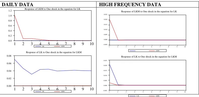
The analysis of the Impulse-Response function of each indices and for both daily and high frequency data, reveals the following results:

DAILY DATA HIGH FREQUENCY DATA

Fig. 1: Impulse-Response Function

If data is daily, a KOSPI shock had a higher impact on the Kospi Midcap index. While the latter is insensitive to a Kospi Midcap shock. For the case of one-minute frequency, a Kospi shock generate a higher impact on the Kospi Midcap index. This is attributed to a lead-lag relationship caused in part by the effect of an non-synchronous trading.

This study, based on impulse response functions, can be supplemented by an analysis of variance decomposition of forecast error. The objective is to calculate the contribution of each of the innovations in the variance of the error. The results for the study of the variance

decomposition are reported in a Table 3. The variance of the forecast error is due to LK for about 99.99% to its own innovations and to 0.01% with those of LKM. The variance of the forecast error is due to LKM 1.3% to the innovations of LK and 98.7% to its own innovations. We can deduce that the impact of a LK shock on LKM is important but there is almost lower than the impact of a LKM shock on LK. For the case of high frequency data: The variance of the forecast error of LK is due to 6% of LKM innovations while that of LKM 26.4% is due to innovations LK. So the impact of a LK shock on LKM is more important than the impact of a LKM shock on LK:

TABLE 3: Decomposition of the variance of the LK and LKM series Daily data

Variance Decomposition of LK:

Period S.E. LK LKM

1 2.03E-09 100.0000 0.000000

2 2.03E-09 99.99713 0.002869

3 2.03E-09 99.99713 0.002869

4 2.03E-09 99.99713 0.002869

5 2.03E-09 99.99713 0.002869

0.0 0.2 0.4 0.6 0.8 1.0 1.2

1 2 3 4 5 6 7 8 9 10

LK LKM

Response of LKM to One shock in the equation for LK

0.00 0.02 0.04 0.06 0.08

1 2 3 4 5 6 7 8 9 10

LK LKM

Response of LK to One shock in the equation for LKM

-0.005 0.000 0.005 0.010 0.015 0.020 0.025

1 2 3 4 5 6 7 8 9 10

LKM

Response of LKM to One shock in the equation for LK

1 2 3 4 5 6 7 8 9 10

L K LKM

Response of LK to One shock in the equation for LKM

(8)

244

6 2.03E-09 99.99713 0.002869

7 2.03E-09 99.99713 0.002869

8 2.03E-09 99.99713 0.002869

9 2.03E-09 99.99713 0.002869

10 2.03E-09 99.99713 0.002869

Variance Decomposition of LKM:

1 2.07E-09 1.306507 98.69349

2 2.07E-09 1.308118 98.69188

3 2.07E-09 1.308118 98.69188

4 2.07E-09 1.308118 98.69188

5 2.07E-09 1.308118 98.69188

6 2.07E-09 1.308118 98.69188

7 2.07E-09 1.308118 98.69188

8 2.07E-09 1.308118 98.69188

9 2.07E-09 1.308118 98.69188

10 2.07E-09 1.308118 98.69188

Ordering: LK LKM

High Frequency data

Variance Decomposition of LK:

1 1.005212 100.0000 0.000000

2 1.008380 94.99944 4.756564

3 1.011948 93.99858 8.891424

4 1.012925 93.99646 5.893540

5 1.013013 93.99468 5.995322

6 1.013046 93.99304 5.996959

7 1.013060 93.99116 5.998837

8 1.013070 93.98931 5.998837

9 1.013079 99.98753 5.998837

10 1.013088 93.98574 5.998837

Variance Decomposition of LKM:

1 0.070037 26.9321 73.09968

2 0.084057 26.8470 73.09915

3 0.089502 26.1678 73.59832

4 0.099497 26.2693 73.59731

5 0.108853 26.3203 73.59680

6 0.115761 26.3644 73.59636

7 0.122618 26.4045 73.59596

8 0.129404 26.4334 73.59567

9 0.135563 26.4569 73.59543

10 0.141370 26.4774 73.5523

Ordering: LK LKM

These results are consistent with those shown by the causality test and impulse response function. In these studies, we can attribute this

(9)

245

attributed to the effect of an asynchronous transaction or delay in the adjustment to new information.

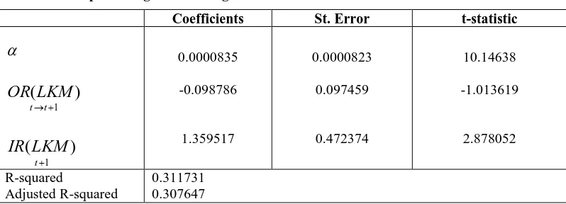
Throughout there results, we propose a simple method of analysis of trading-break and post-trading break in order to infer whether such predictability is attributed to a non-synchronous trading or delayed price adjustment. From the estimation of VAR (3), we found that the first three minutes of Kospi lags are significant in determining the value of the KospiMidcap. In what follows, we estimate by OLS the equation linking the Kospi1 overnight return, KospiMidcap2 overnight return and the first three minutes returns of KospiMidcap of the trading day following:

1 1 1

)

(

)

(

)

(

    





t t t t t

LKM

IR

LKM

OR

LK

OR





1 (close) day t in returns ndex (close) day t in returns ndex -(open) 1 day t in returns ndex i i i  2 00) : 9 (at 1 day t in returns ndex 00) : 9 (at 1 day t in returns ndex -03) : 9 1(at day t in returns ndex    i i i Where : 1

)

(

 t t

LK

OR

: The Kospi overnight between day t

and t+1; 1

)

(

 t t

LKM

OR

: The KospiMidcap overnight

between day t and t+1;

1

)

(

 t

LKM

IR

: KospiMidcap first three minutes

of a day t;



: is a constant;



: is an error.

(10)

246

TABLE 4: Kospi overnight return regressions

Coefficients St. Error t-statistic



1

)

(

 t t

LKM

OR

1

)

(

 t

LKM

IR

0.0000835

-0.098786

1.359517

0.0000823

0.097459

0.472374

10.14638

-1.013619

2.878052

R-squared

Adjusted R-squared

0.311731 0.307647

The regression indicates that Kospi overnight return is more correlated with KospiMidcap of three first minutes. The lead-lag effect is attributed to an non-synchronous trading or a delay in price adjustments to the "news". The same conclusion is presented by Lo and Mackinlay (1990). These authors found that portfolios of smaller stocks are characterized by a high level of autocorrelation cannot be explained by a non-synchronous trading alone, and therefore one cannot rule out the presence of actual lead-lag effects running from larger to smaller stocks in addition to non-synchronous trading effects (Camilleri and Green, 2004)

Conclusion

The purpose of this chapter is to study the effect of an non-synchronous trading on the predictability of returns Korea stock exchange via the examination of the lead-lag effect. Three methodologies were adopted on daily and high frequency data of two indices. These are different levels of liquidity based on bid-ask spread. Specifically, in the high-frequency data, the results show that the more liquid index leads the less liquid. Several authors have associated this lead-lag either an asynchronous transaction or delay price adjustments to new information. To show how these two causes of predictability is more relevant in explaining the lead-lag effect, we analyzed the returns during a trading –break period and we got the persistence of lead-lag effect. In this case, such predictability cannot be attributed to delays in price adjustments on the part of investors that during the overnight market participants had sufficient

time to adjust their expectations. Therefore, we conclude that the lead-lag effect is mainly caused by an asynchronous transaction and that this predictability will not likely be abnormal profits. In addition, based on previous studies, the asynchronous transaction is not the main

cause of predictable returns. Moreover, the fact

that stock prices contain predictable components does not necessarily imply that predictability is economically significant and this need not be a symptom of market inefficiency.

References

Boudoukh, J., Ridchardson, M. and Whitelaw. R. (1994). Industry Returns and the Fisher Effect. Journal of Finance, 49: 1595-1616.

Camilleri, S. J. and Green, C. J. (2004). An analysis of the impact of non-synchronous trading on predictability: Evidence from the National Stock Exchange, India. SSRN G12, pp.1-50. Cohen, K., Maier, S., Schwartz, R. and

Whitcomb. D. (1979). On the existence of serial correlation in an efficient securities market. TIMS Studies in the Management Sciences, 11: 151-168. Fisher, L. (1966). Some new stock indexes.

Journal of Business, 39: 191-225. Granger, C. W. J. (1969). Investigating causal

relations by econometric methods and cross spactral methods. Econometrica, 37: 424-438.

(11)

247

synchronous Trading. Journal of Econometrics, 45: 181-211.

Lo, A. and Mackinlay A. C. (1990b). When are contrarian profits due to stock market overreaction. The Review of Financial Studies, 3: 175-205.

Mills, T. C. and Jordnov. J. V. (2000). Lead-lag patterns between small and large size portfolios in the London Stock Exchange. Applied Financial Economics, 8: 167-174.

Sâfvenblad, P. (1997). Trading volume and autocorrelation: Empirical evidence from the Stockholm Stock Exchange. Working Papers Series, Economics and Finance, pp.1-28.

Schotman, P. C. and Zalewska, A. (2006). Non-Synchronous trading and testing for market integration in Central European emerging markets. Journal of Empirical Finance, 13: 462-494.

APPENDIX

TABLE 1: OLS estimation of VAR equations (daily data and high frequency data)

OLS estimation of a single equation in the unrestricted VAR

Dependent Variable: LOG Kospi(LK) Method: Least Squares

Sample(adjusted): 02/01/2004 05/02/2008

Included observations: 1016 after adjusting endpoints

Regressor Coefficient Std. Error t-Statistic Prob.

Constante 0.0064 0.00247 3.5549 0.0000

LK(-1) 0.0095 0.0316 -0.3009 0.7635

LKM(-1) -0.0007 0.0309 -0.1704 0.8647

R-squared 0.000131 Mean dependent var 6.37E+09

Adjusted R-squared -0.001843 S.D. dependent var 2.03E+09

S.E. of regression 2.03E+09 Akaike info criterion 45.70184

Sum squared resid 4.17E+21 Schwarz criterion 45.71638

Log likelihood 2323.53 Durbin-Watson stat 2.001528

Fstas 4.1025[0.035] System LogLiklihood 4644.090

Diagnostic tests

Test Statistics LM version F version

A : Serial Corrélation 5.338193 [0.228] F(1, 1015)=5.345261 [0.220]

B : Normality 170.062 [ 0.0000] Not applicable

C : Heteroscedasticity 33.096964 F(1, 1015)=120.772786 [ 0.5429]

A : Lagrange Multiplicateur Test of residual serial correlation B : Based on a test of skewness and kurtosis of fitted values

(12)

248

Dependent Variable: LOG kospI(LK) Method: Least Squares

Sample(adjusted): 21/01/2008 25/01/2008

Constante 0.3571 0.7862 6.8130 5.3571

LK(-1) 0.0794 0.0386 2.0572 0.0794

LK(-2) 0.0780 0.0386 2.0218 0.0780

LK(-3) 0.0310 0.0386 0.8043 0.0310

LKM(-1) 0.0341 0.5229 0.0653 0.0341

LKM(-2) 0.0170 0.6393 0.0267 0.0170

LKM(-3) 0.0341 0.5229 0.0653 0.9479

R-squared 0.0173 Mean dependent var 740.92

Adjusted R-squared 0.0085 S.D. dependent var 1.0147

S.E. of regression 1.0104 Akaike info criterion 286.89

Sum squared resid 685.08 Schwarz criterion 291.55

Fstas 19.715 [0.000] System LogLiklihood 4644.090

Diagnostic tests

A : Serial Corrélation 3.2145 [0.311] F(1, 1850)=3.5371[0.060]

B : Normality 566.01[0.0000] Not applicable

C : Heteroscedasticity 520.08[0.000] F(1, 1850)=853.1230 [ 0.000]

C: Based on the regression of squared residuals on squared fitted values.

Dependent Variable: LOG kospi Midcap(LKM) Method: Least Squares

Sample(adjusted): 02/01/2004 05/02/2008

Constante 0.00637 0.00280 2.275409 0.0000

LK(-1) -0.00660 0.03227 -0.206138 0.8367

LKM(-1) 0.0175 0.03162 0.555299 0.5788

R-squared 0.0003 Mean dependent var 6.44E+09

Adjusted R-squared 0.0016 S.D. dependent var 2.07E+09

S.E. of regression 2.07E+09 Akaike info criterion 45.742

Sum squared resid 4.34E+21 Schwarz criterion 45.756

Fstas 15.258[0.000] System LogLiklihood 4644.090

Diagnostic tests

B : Normality 351.1496 [ 0.0000] Not applicable

C : Heteroscedasticity 75.83201 [0.0000] F(1, 1015)=58.4308 [0.0000]

(13)

249

Dependent Variable: LOG Kospi Midcap(LKM) Method: Least Squares

Sample(adjusted): 21/01/2008 25/01/2008

Constante 5.5393 5.4784 1.0111 0.3123

LK(-1) 0.0001 0.0026 0.0469 0.0266

LK(-2) 0.0001 0.0026 0.0457 0.0369

LK(-3) 0.0001 0.0026 0.0446 0.0444

LKM(-1) 0.6636 0.0364 18.212 0.0000

LKM(-2) -0.0015 0.0445 -0.0340 0.9728

LKM(-3) 0.3302 0.0364 9.0646 0.0000

R-squared 0.9751 Mean dependent var 766.274

Adjusted R-squared 0.9749 S.D. dependent var 0.4450

S.E. of regression 0.0704 Akaike info criterion 245.89

Sum squared resid 3.3257 Schwarz criterion 241.226

Fstas 43.96304 [0.000] System LogLiklihood 4644.090

Diagnostic tests

B : Normality 572.057[0.0000] Not applicable

C : Heteroscedasticity 99.2016[0.0000] F(1, 1850)=99.368[0.0000]