Article
Rebound Effect and Technical Learning of
Energy-environmental Evaluation in Manufacturing Industry
Jiang Wang 1, Kunyue Wang 2 and Lijuan Wang 3,*
1 Beijing University of Chemical Technology,Beijing, China; [email protected] 2 Huazhong Agricultural University,Wuhan, China; [email protected]
3,* China National Center for Human Resource, Beijing, China; Correspondence: [email protected]; Tel.: +086-13121608203
Abstract: We introduce a total energy and environmental evaluation method in the manufacturing industry. The method gives us a series of descriptive indexes to assess the overall environmental effect level on materials, energy, wastes and products in the life cycle process. Meanwhile, the method uses partial indexes, environmental effect factors, and correction offsets into the quantitative model to analyze the learning process and rebound effect on the energy and environment at each procedure. In this work, we choose S-shaped learning curves to describe how to decrease energy consumption and improve the technical learning by doing for recent 30 years. Also, we draw the different rebound effect curves of the total energy-environmental evaluation with technical learning method, which use the annual industrial production growth rate to show that it's significant to estimate its effect on technology changes. The ideas about the interaction of energy and production environment from material flows to energy consumption, direct us to build an example to estimate quantitatively the results with different condition factors, and realize the process improvement and develop new products.
Keywords: energy-environmental evaluation; cleaner production; descriptive index; technical learning curve; rebound effect; life cycle
0. Overview
The environmental effect assessment of the manufacturing process and its equipment, is a relatively new research area. In order to promote manufacturing enterprises to act on technical learning of cleaner production and decrease environmental impact, we provide an energy-environmental effect evaluation method in the life cycle process, use an example to analyze the environmental effect in manufacturing industry, and assess its cleaner production technologies and rebound effect.
1. Introduction
Traditional researches on assessment methods mainly have adopted the environmental impact assessment (EIA) of the production process or the environmental impact assessment of the product (equipment) life cycle [1-6]. Commonly the cleaner technologies are closely on process control of the life cycle of products, so that recently there are more efficient energy technologies and friendly environment technologies to use in industries, such as using secondary energy and wastes recycling. And in this paper, we introduce the environmental impact factors, the learning fraction and rebound effect factors into the total evaluation model to simulate the change of energy-environmental impact over the life cycle from the beginning raw material preparation to the end of production.
In the researches, the secondary energy effect, that always derive from how an industry adapts itself to a particular cleaner technology, may be more positive through technological learning and even exceed the energy saving limit of primary energy using. Sondes [7] affords an overview and a critical analysis of the technological learning concept and the energy–environment–economy model
considered with technological learning method. Traditionally, Computable General Equilibrium (CGE) model assumes that energy efficiency improves at a constant rate over time, but this fails to capture some characteristics of endogenous technical change such as learning by doing and learning by researching.
The Technical learning curve (TLC) is another widely used technique to represent the indicators of technological performance and experience. This theory is usually attributed to J. P. Wright [8], which performance indicators are mainly the capital costs, investment costs, production costs and the prices that is a proxy of costs in some cases [9-12]. Its experience performance indicator is the cumulative capacity or production, and normally its model is expressed to an exponential regression function by the one-factor learning curve (OFLC) [13]. Dudley [14] tries to use the technical characteristics in a particular sector of a developing economy entity to simulate the process of technical change and suggests that technical learning depends on the cumulative output and the production time. Carr and Yelle propose S-shaped learning curves to make the model more powerful and flexible to capture the observations about the primary transient phase and saturation phase [15,16].
For the classification of rebound effects of energy efficiency, Khazzoom and Greening define the direct rebound effect and Jevons defines indirect rebound effects [17-19]. And both effects represent the overall economy-wide rebound effects in the process. To assess the rebound effects on energy-environmental technical learning, Greening et al. [20] refer to the factor of productivity growth, but which it is to know as an opposite factor in Jevons’s [19] thesis (rebound greater than 100%) . Sorrell affirms that the rebound effects will weaken the effectiveness of energy policies [21], and the more time and the more widening of the system boundary for the dependent variable (energy consumption) will increase the rebound effects. Indeed, the increase of energy consumption in industrial societies over the past 21 century may partly use technologies to save time, and this allows producers to complete faster through using the cost of more energy.
2. Assumption and Methods’ Fundamental Study
2.1. Assumption
This paper's energy-environmental evaluation method is a kind of interactive, quantitative analysis of environmental impacts of material flows and energy flows in production process. This method combines the elements of raw materials, wastes and products into the energy model to represent the process’ environmental characteristics [22]. In this model, the energy unit covers consumption and reuse of major energy sources, and the materials unit responds the properties of raw materials and quantitative data of intermediate materials in manufacturing production. Because the real material flows are complicated in the production process, in the model we choose the simplified input-output method to express the product output at each procedure, relatively more clear to outline procedure characteristics academically, that is to set up a standard output of materials. The wastes unit of the model figures out their characteristics of recycling and production at each procedure that there exists wastes to generate in. From the above mentioned parts, we describe step by step the flow process of materials and energy in manufacturing production.
In general, for rapidly developing countries, the scale effect will increase pollution and other discharge, overwhelm the time effect. Since rebound effects are very difficult to quantify in manufacturing industry, it adopts the factor of annual industrial production growth rate (AIPGR) in this energy-environmental evaluation model, to assess the potential rebound impact of learning by doing. It seems that reducing emissions of most pollutants and control of waste disposal are rising with productivity, and furthermore the factor lets us obtain a more realistic view about the effect of technological changes on environmental quality.
2.2. The energy-environmental evaluation index Wz
previous researches to estimate these impacts [5,22]. We express the energy-environmental evaluation index Wz as a linear mathematical regression index in the overall descriptive model, that means Wz is square root of square sum of these descriptive indexes, see the following Formula (2.1):
( ) ( ) ( )
2 2 2( )
2W
z=
W
s+
W
e+
W
o+
W
p.
(2.1)Wz indicates a risk factor of overall energy and environment of cleaner technology, and its results can divide into four schemes, such as The lower (Wz<10), Low (10≤Wz<15), High (15≤Wz<20) and The higher (Wz≥20), to check the environmental impact degree of clean technology in the process.
3. Technical Learning Method
To judge the whole energy-environmental impact of technologies' life cycles by technical learning method, this paper discusses how the learning curve of Index Wz decreases from the early higher impact degree to the last lower one along with learning by doing. In those pervious researches on manufacturing industries, Baloff [23] compares with the learning parameters of 17 startup firms and presents how to vary into different patterns. Even though there are very different patterns at the same production line, it can help us to visualize the different learning processes over time, and meanwhile for decision makers, it will outline the latest technological mature trends. Another example is that Kar [24] gives a whole view of learning curve approach at a manufacturing level and builds cost model to understand the process more.
3.1. Wright's learning curve
The classical learning curve is from Wright's study [25], in which Wright's learning curve describes how to use a predictable pattern to decrease the average cumulative labors for an aircraft production line [24]. It covers that when the volume of production is doubled how to build an exponential learning model to improve a process.
3.2. S-shaped learning curve
Wright's work extends the application of learning curve to reveal the technical learning trends in different industries and predict these technologies' future costs. Originally the researchers [15,16] provide an S-curve with a different process variable and cumulative production volume, to learn and track the process variation during the production time. An S-curve requires four parameters to define its shape, instead of the traditional simple log linear method with two parameters. This paper accepts the S-shaped learning curve to capture technology variation more powerfully and flexibly. Choose a non-dimensional learning fraction y* (see Formula 3.1) to represent the trends of process variable over learning time:
y*=(W-Wmin)/(Wmax-Wmin) , and 0≤ y* ≤1 . (3.1)
Where:
y* - The learning fraction,
W – The process variable, in this paper equal to the total evaluation index Wz, Wmin - The minimum value of W, while the learning fraction y* is 0,
Wmax - The maximum value of W, while the learning fraction y* is 1.
The non-dimensional learning fraction y* varies between 0 and 1, that is easy to transform ELCs (Early Learning Curves) with different parameters to a normalized equation to describe the learning cycle of cleaner technologies. Firstly to treat the normalized cumulative volume V* by the following formula (3.2):
V*= V/ Veq, (3.2)
y*=1/(1+e(αV*+β)), (3.3)
Where:
α, β – Constants,
V* – The normalized cumulative volume.
To define the S curve's four parameters (the max value, the min value, α and β), this paper refers to a given set of the limited values for the long-term cycle to obtain the simple inspection [15,16]. Only the parameters α and β are not easy to define the shape of learning curve because the two parameters requires a regression analysis of the data. For example, we can get a fast learning process when within half equipment life 95% learning completes and within 0.01 equipment life 5% learning completes , and then this leads to the following values: α = 11.801 and β = -2.956. Similarly, we can define a slow learning process when 95% learning is completed within one full equipment life and 5% learning is completed within 0.01 equipment life, and then this leads to the following values: α = 5.948 and β = -3.004. To set up the learning cycle, we substitute the normalized cumulative volume equation (3.3) into the learning fraction y* of the S-shape learning curve equation (3.1) , and then get the total index Wz expression with four parameters, see as the following formula (3.4) :
Wz=Wz,min+[1/(1+ e(αV*+β))]*(Wz,max-Wz,min). (3.4)
3.3. Total environmental evaluation index with learning by doing
This paper discusses four conditions of environmental evaluation index according to different environmental factor or secondary effect: Condition A includes environmental factor and secondary effect; Condition B includes only environmental factor; Condition C includes only secondary effect; Condition D includes neither of them.
To Condition A, we can have the minimum Wz value of total environmental evaluation index from Formula (2.1), reflecting the effects of environmental factors and secondary energy resources. The environmental impact degree of Condition A is lower than Condition D, that doesn't take account
of secondary energy resources and waste recycling,while
z
ewiandm
wij are 0 and k=1, and itsdetails can derive from the following formulas (3.5a-3.5e):
(
) (
) (
)
(
)
2max , 2 max , 2 max , 2 max , max ,
W
z=
W
s+
W
e+
W
o+
W
p,
(3.5a)Where:
=
=
n i cp sij sm
m
1 2 max ,W
,
(3.5b)
=
=
n i cp ei e em
z
c
W
1 max,
,
(3.5c)
= =
=
m i n j sj sij om
m
W
1 1 2 max, , (3.5d)
= =
=
m i n j sj sij cp pi pm
m
m
m
1 1 2 max ,W
.
(3.5e)For observing the secondary effect, this paper discusses Condition B and Condition C to analyze the effect of secondary resources on the energy-environmental model. To Condition B, its environmental impact degree is a little poorer than Condition A's. We get the minimum process variable Wz from equation (2.1) where there are secondary resources to recycle and the practice environmental impact factors to share(k<1), and define the value of process variable Wz under
Condition B from equation (2.1) while
z
ewiandm
wij are 0 and the environmental impact factors arein practice.
Moreover, to Condition C, the estimated environmental impact degree is a really higher level than the above condition A and a little bit lower than Condition D’s, thus its total energy -environmental evaluation model chooses secondary energy resources to simulate without the environmental impact. Then we get the value of process variable Wz from equation (2.1), which is to keep the environmental impact factors out of the simulation model (k=1) and adds the secondary effect factors, seeing the following equations (3.5f-3.5h):
=−
=
n i cp ewi ei em
z
z
W
1 max,
,
(3.5f)
= =
−
=
m i n j sj wij sij om
m
m
W
1 1 2 max,
,
(3.5g)
= =
−
=
n i n j sj wij sij cp pi pm
m
m
m
m
1 1 2 max ,W
.
(3.5h)4. Rebound Effects of Learning Curve Wz
The importance of rebound effects may increase over time as manufacturing saving energy technologies and their learning behavior adjust. Sorrell [26] believes in developing countries, the unsaturated market enthusiastically takes up the technology innovation and more productivity that result the larger rebound effects [21]. Some argue that rebound effects are of minor importance for most energy services [27,28]. Others argue that they are sufficiently important [29,30]. For the engineer, they insist that a set of given technologies or activities makes an increase in the productivity and hence there is no rebound effect [31]. This paper defines that the system boundary of rebound effects is of the manufacturing sector where they're materials (raw materials, products and wastes) or energy in the analyzed process to assess the various rebound effects of total energy-environmental impact in a special long time along with the increase of productivity.
To the manufacturing industry it isn't easy to get the replacement effect, thus these changes in the technical effects of productivity over periods are not easy to predict. It's therefore simple to assume fixed and constant technical coefficients, which assumption is operationally convenient, but it will clearly call for improvement when we come to check the predict data.
4.1. Relative principles of annual growth rate
4.2. Annual industrial productions growth rate
We want to get the relatively real growth rate of annual industrial productions with rebound effects. From the above discussions, we know the more technical change government investigate, the higher production growth rate will have, and then enlarge the learning effects of the technical changes from annual productions. Therefore, we choose an annual industrial productions growth rate, and see the following formula (3.6):
= −
+
−
−
=
ni i i
i i AIPGR
W
W
W
W
n
1 11
1
W
,
(3.6)Where:
Wi+1- A growth rate at analyzed year i+1,
Wi - A growth rate at analyzed year i,
Wi-1- A growth rate at analyzed year i-1,
n - Number of years in the period,
WAIPGR- The annual industrial productions growth rate.
4.3. Rebound effect of normalized cumulative volume V*
Since the original normalized cumulative volume V*, that calculates from formula (3.2), enlarge the energy-environmental impact without considering the rebound effect, We can get the decreased V* to reflect the rebound effect, according to the above discussion of annual industrial production growth rate, see the following formula (3.7):
)
W
1
(
*
* *
AIPGR re
R
V
V
=
−
•
,
(3.7)Where Rre – A percentage rate of rebound effect.
5. An Experimental Example of Steel Industry
This section may be divided by subheadings. It should provide a concise and precise description of the experimental results, their interpretation as well as the experimental conclusions that can be drawn.
5.1. Recent life cycle data
This paper estimates the process of 1 Kg hot-rolled steel production, which includes raw materials preparation, energy consumption and recycling, key procedures and their intermediary products and wastes, and we can see Table 1 and Table 2. To the current process of steel production, its total energy consumption is expressed as a standard fuel quantity to simplify the descriptive energy-environmental model in this paper. The more secondary energy recovery and utilization, the less Wz would have. To set the correction coefficient of energy unit index We equal to 10, then we can predict that the energy effect on the total energy-environmental model is obviously outstanding.
Table 1. Raw materials of 1Kg hot rolled steel production [32], Unit:Kg.
No. i Raw material Weight kj
0 Iron ore mining 2.89 0.2
1 Manganese ore 0.05 0.2
2 Limestone 1.7 0.2
3 Coke 1 0.2
4 Water 1.67 0.3
5 Dolomite, fluorite 0.03 0.2
6 Oxygen 0.68 0.5
Table 2. Data of energy, resources, secondary energy recovery and environmental impact factor for production of 1Kg hot-rolled steel [32].
No. i Procedure Energy consumption, Z
ei, KJ/Kg
Material outputs, g/Kg
Secondary energy [33], KJ/Kg
CO2 emission [34], g/Kg ki
1 Iron ore mining 2629.27 2887 230.95 0.08
2 Iron ore cleaning 259.16 1154.7
3 409.09 1473.9 11.723 0.01
4 Lime production 418.83 104.4 123.19 0.04
5 Sintering 3338.6 1426.2 191.93 0.07
6 Coking 6195.04 1052.8
Coking gas, 2230.2 Coal moisture
control, 17.6
493.48 0.18
7 Iron making 2177.31 1296.4 Blast furnace gas,
1138.6
1457.12 0.52
8 Steelmaking 791.87 1159.9 Converter gas, 460.8 15.34 0.01
9 Continuous casting 3439.03 1110 42.088 0.02
10 Hot rolling 2696.81 1000 234.98 0.08
Total 22355.01 2800.8
To calculate the energy unit index, it needs the thermal physical properties of billet, seen the reference published by Wang [35]. In the practice initial temperature of billet at heating furnace is divided into 2 kinds: one is hot charging with 650℃, and another is cold charging with 270℃. See Table 3, when we give 80% hot charge rate and 1050℃ final billet temperature, the total energy consumption is 2696.81 KJ/Kg at hot rolling procedure, and the secondary energy is 9.34% of total thermal energy during the mixed hot and cold charging process. Then the most secondary energy is 412.55 KJ/Kg when all slabs are put into heating furnace with zero hot charge rate at hot rolling procedure.
Table 3. Secondary heating energy Zewi of Carbon steel at hot rolling.
Hot charge rate,% 100 80 60 40 20 0
Zewi , KJ/Kg 211.57 251.76 291.96 332.16 372.36 412.55
Zewi / Zei ,% 7.85 9.34 10.83 12.32 13.81 15.3
To 1Kg hot-rolled steel, its waste data includes waste gas, waste liquid and solid wastes, seen Table 4. Recently there have been the massive solid wastes to recycle as secondary resources into the manufacturing process. To keep the example value of waste unit index easy to compare with the other partial indexes, this paper adopts the percentage value of wastes in the waste unit model.
Table 4. Data of wastes at main procedures for 1Kg hot-rolled steel [36], Unit: %.
No.I Procedure CO2 SO2 CO SS COD Dust Particulate
matter
Solid wastes
Reutilizing ratio of solid wastes
1 Iron ore mining 8.2 68.5 98.7 92.8 82.6 25.5 8.2
2 Coal mining 0.4 1.5 0.1
3 Lime production 4.4 0.1 11.5
4 Sintering 6.9 15.0 2.6 7.9 10.3 42.3 30.4 60
5 Coking 17.6 7.8 0.2 0.1 12.7 0.6 14.0 0.1
6 Ironmaking 52.0 0.1 4.0 25.4 1.8 28.2 21.5 91.4
7 Steelmaking 0.5 0.3 0.1 0.1 31.7 0.9 7.0 6.7 94.0
8 Continuous
casting 1.5 2.4 0.1 0.2 0.8 0.1
9 Hot rolling 8.4 5.9 0.8 0.2 22.2 1.6 8.5 4.1 95.0
Total,Msj, g/Kg 2800 51 110 120.5 0.282 295 45 1950
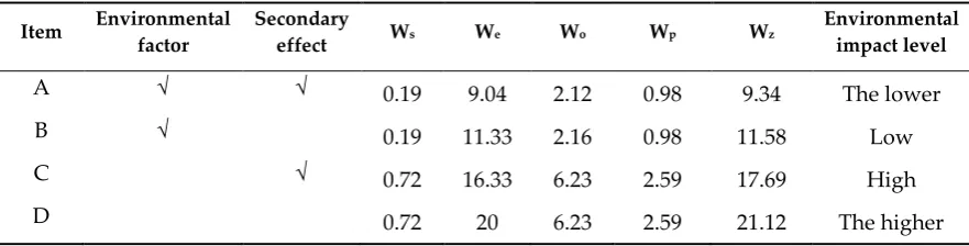
Under different factors, Table 5 lists the relative estimated indexes of cleaner technology from formula (2.1), to show that the overall degrees of energy and production environmental impacts in steel process. Comparing condition A to condition B, the secondary effect rate of Wz is about 19% and Comparing condition C to condition D, the rate is about 16%, lower than the first group, that means under the influence of environmental factor, the secondary effect rate of Wz is more positive in the steel industry, to let us pay more attention to this effect.
Table 5. Estimated environmental evaluation indexes from formula (2.1) under different conditions.
Item Environmental factor
Secondary
effect Ws We Wo Wp Wz
Environmental impact level
A √ √ 0.19 9.04 2.12 0.98 9.34 The lower
B √ 0.19 11.33 2.16 0.98 11.58 Low
C √ 0.72 16.33 6.23 2.59 17.69 High
D 0.72 20 6.23 2.59 21.12 The higher
5.2. Wz learning curves
In the previous researches, Dudley (1972) gives a measure of learning with the annual rates of growth and estimates 65% learning rate in the foundries with 51% actual productivity change. To analyze Wz learning procedure, this paper describes the experience curves of steel industry production, while there are 80% hot charge rate and 30 years economical life cycle between 1980 and 2010. And further through learn by doing, the S-curve parameters of Wz are given as: Wz,max = 21.12, Wz,min = 9.34 where α = 5.948 and β = -3.004 at slow learning rate. So Equation (3.4) is changed into the following expression:
Wz=9.34+[1/(1+exp(α*V/500000+β))]*(21.12-9.34) .
Figure 1. Wz learning curves at fast learning rates, data from www.worldsteel.org.
Our research indicates that for manufacturing productions it takes serious risks to shorten a learning cycle, which is inherently cumulative [23]. Ultimately, choosing to describe the learning curves by learning by doing, might be particularly relevant to the capital intension of industries [37]. Worker's learning by doing in metal working would be primarily a function of time, due to the production tasks. So Dudley estimated that percent change in steel productivity is 37% [14].
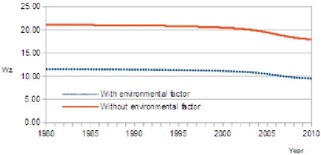
5.3. Secondary effects on Wz learning curve
To analyze secondary effects, seeing Table 5, this study sets two states: one is from initial condition A to final condition B, and another is from initial condition C to final condition D, to get Wz learning curves with secondary effects in the steel industry, see Figure 2. From two curves and estimated results, we can learn that the first Wz learning values with environmental factors change more smoothly and highly than the second curve among the annual 30 years. It means that the secondary effects with environmental factors have actively reduced to the lower learning field of Wz and reflect the more positive learning effect comparing without environmental factors. The more secondary resource utilization, the Wz learning curve is lower than the state without resource recycling. We may use Wz learning curve to balance learning level of cleaner technology and adjust environmental impact degree for steel process.
Figure 2. Secondary effect on Wz learning curve, data from www.worldsteel.org.
We normally express rebound effects as a percentage of the expected normalized cumulative volume V* from an energy-environmental improvement. In general, if we take enough impact on whole energy and environment for a new energy-efficient technology as the dependent variable, then the estimated rebound effect is larger. Jevons cites the example of the Scottish iron industry, where the reduction of the coal consumption will have a tenfold increase in total consumption [19]. More recently, Rosenberg [38] has cited the comparable steelmaking example, that the low-cost Bessemer steel initially facilitates the growth of the rail industry. However, the British economist, Len Brookes, takes up with Jevons’ arguments [39,40]. In his 1984 paper, Brookes quotes Sam Schurr’s observation that it is energy to drive modern economic systems instead of a demand for energy [40]. Since technical change typically improves the productivity of several inputs simultaneously, Saunders [41] demonstrates the potential larger rebound effects and investigates the effect of improvements in energy productivity [42] .
In recent modelling studies, Sweeney [43] puts the long-run, rebound effect for primary energy in the range -0.25 to -0.6. In contrast, Kaufmann [44] uses econometric analysis to propose a range from -0.05 to -0.39. A lower rebound effect value may show a potential larger rebound effects. By combining the estimates of embodied energy and secondary effects, it can get an estimate of the total indirect rebound effect. The available studies suggest that economy-wide rebound effects may often exceed 50%.
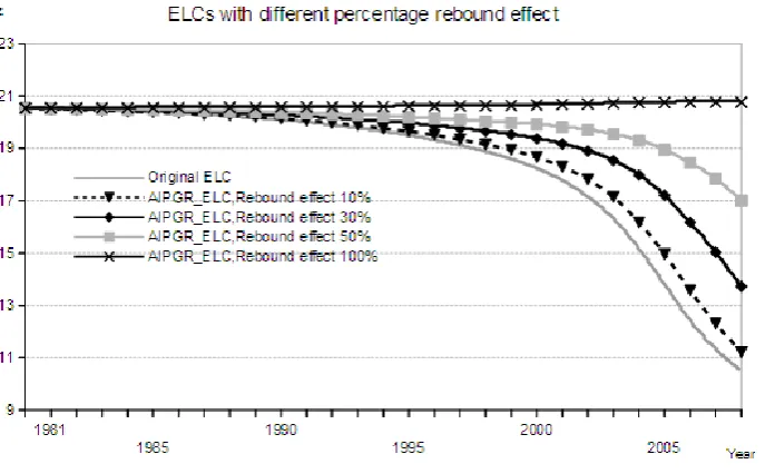
This paper gives the original environmental learning curve (ELC) and its different rebound effects learning curves that simulate in annual industrial production growth rate method, see Figure 3. In this example, when the range of rebound effect is 100%, the rebound effect will submerge the environmental improvement of the clean technologies learning, that means the environmental policies will lose their usages. We also can see that ELC appears shape change from the original S-shape to a line and meanwhile there is more increase level at the final of analyzed time. When the percentage of rebound effect is 30%, the shape of ELC appears smoothly S-shaped, similar to the original ELC, its last Wz is 13.73, increase about 30% compared with the last Wz 10.48 of original ELC, so we know that rebound effect deeply changes the environmental learning process according to 30 years data in China.
Figure 3. ELCs with different percentage rebound effects
6. Conclusions
this paper gives a recent example of the environmental evaluation approach of clean technology in the steel industry to estimate the overall environmental impact of steel process and its products.
We extend the energy-environmental model to let it mixed with traditional S-shaped learning theory, and simulate Wz learning curves among 30 years to analyze comprehensively the total energy-environmental impact and secondary effects on steel industry, where the generated results data are from the whole life cycle of steel process.
We predict the different rebound effect curves of the total energy-environmental evaluation with technical learning, which indicate that it's significant to cut its estimated rebound effect on cleaner technologies. The results show that rebound effect has deeply changed the environmental learning process according to 30 years data in China.
The data of waste index of the energy-environmental evaluation model in this paper include information of current main cleaner technologies in the steel industry, such as waste gas recycling and utilizing, and secondary solid waste resource. The data of energy index includes secondary effect of thermal process.
We use the evaluation method to quantitatively analyze the cleaner technical learning for multiple processes in manufacturing industry, so as to carry out process changes and new product development under the purpose of cleaner technology. We also can use this evaluation method for industry managers to understand the importance of energy saving and material recycling utilization.
Funding: This research was funded by NATIONAL SOCIAL SCIENCE FUND PROJECT, grant number 17BGL267.
Acknowledgments: We thank the comments from the reviewers and editors are sincerely acknowledged..
Appendix A
A.1. Raw material unit index
The descriptive raw material index WS include most of the raw materials involved in current
manufacturing production (except for raw materials recycling). These raw materials have ores, coal, main auxiliary materials and water for cooling, for an example, we calculate the raw material unit index WS its factor as the following formula (1):
=
=
=
ni cp
sij
j j s
m
m
k
1
2 3
1
W
(1)
Where:
sij
m
- A quantity of raw material j at procedure i,cp
m
- A total volume of material or energy in the process,j
k
- An environmental impact factor of raw material j, of which separate it into 3 kinds: solid0.2, liquid 0.3 and gas 0.5.
A.2. Energy unit index
When we assess the current energy consumption, the energy unit index We is a total energy consumption to directly act on the normal or thermal process in the industry and relate to procedure consumption. And then when we describe its economic effects, all energy materials (solid, liquid and gaseous fuels), electricity and thermal energy in the production express as the calorific value (=29.3076 MJ/kg) that is a standard coal fuel. The following formula (2) calculates the energy unit index We and its factors:
(
)
=
−
+
=
ni cp
ew ei i e
e
m
z
z
k
c
W
1
i
1
(2)
e
c - Correction coefficient of energy unit index,
i
k - CO2 emission ratio at procedure i ,
ei
z
- A total volume of energy consumption at procedure i, expresses as a standard fuel quantity,ewi
z
- An amount of secondary energy at procedure i, expresses as a standard fuel quantity.We take the secondary energy unit index at each procedure into account of the temperature fluctuation for intermediate products at heating furnaces where we reheat them at the required temperatures and let them suitable for hot making. The formula (3) shows the estimated heat Q:
( )
(
0)
' '
t
t
c
m
t
Q
=
−
(3)
Where:
Q
- A heat function of second energy consumption of intermediate product,m
- A weight of intermediate product,c
- A specific heat of intermediate product,0
t
- An initial temperature of intermediate product in a heating furnace,'
t
- A heating temperature of intermediate product.For matrix function Q (t'), there are different material components and initial temperatures of intermediate products from Casting Machine M to Heating Furnace N, the following formula (4) calculates an overall energy consumption at heating procedure :
( )
= n m j m m j i i n j Q Q Q Q Q Q Q Q t Q , , 1 , , 1 , , 1 , 1 1 , 1 ' ... ... ... ... ... ... ... ... ... ... ... ... ... ... ... ... ...(4)
Where: j iQ
, - A heat function of intermediate product from casting machine i to heating Furnace j, whenwe estimate the secondary energy consumption.
Then, formula (5) expresses an average amount of secondary heat energy at each procedure, directly derived from the sum of heating consumption of intermediate products:
( )
i j Q Z m i n j j i ewi=
=1 =1
,
(5)
A.3. Waste unit index
When we describe these wastes academically, the waste unit index Wo covers most of pollutants taken away from each procedure in the industry. And most importantly, there are waste gases to discharge into the atmosphere, such as sulfur dioxide, CO, CO2 and etc.; waste waters to flow out
into rivers, such as suspended liquids and COD; and solid wastes to pile up on the grounds or diffuse into the air, especially including various particles, such as dusts, smokes, slags and other things like sediments. The following formula (6) calculates the waste unit index Wo and its factor:
= = =
−
=
p mi n j sj wij sij s o
m
m
m
k
W
1s 1 1
2
(6)
Where:
s
sij
m
- A quantity of waste j at procedure i,wij
m
- An utilization rate of secondary waste j at procedure i,sj
m
- A total volume of wastes at procedure i.A.4. Material unit index
When we describe the material flows at each procedure, the material unit index WP contains a
negative environmental effects of product flows into its mathematical model. It is relatively convenient to estimate a total material output at each procedure as a standard value. In the below formula representation, we adopt an Index kpi as a risk factor of environmental impacts to assess
material flows and their emissions at each procedure, equal to 10% combined effects of wastes where Chapter A.3 has discussed. The following formulas (7) gives the material index unit WP and its factor:
(
)
=
=
ni
pi pi
p
w
k
1
W
(7a)(
)
21 1
2
W
= =
−
=
ni
m
j sj
wij sij s
cp pi p
m
m
m
k
m
m
(7b)
Where:
pi
m
- A quantity of material flow at procedure i,pi
k
- An equal value of the combined effects of wastes.References
1. Hunt, R.G.; Sellers, J.D.; Franklin, W.E. Resource and environmental profile analysis: a life cycle environmental assessment for products and procedures. Environmental Impact Assessment Review 1992, 12, 245-69.
2. Bisset, R. Developments in EIA Methods, Environmental Impact Assessment: Theory and Practice; Publisher: Unwyn Hyman London, UK, 1998.
3. Morris, P.; Therival, R. Methods of Environmental Impact Assessment; Publisher: UCL Press Ltd London, UK, 1998.
4. Dijkmans, R. Methodology for selection of best available techniques (BAT) at the sector level. Journal of Cleaner Production 2000, 8, 11-21.
5. Fijal, T. An environmental assessment method for cleaner production technologies. Journal of Cleaner Production 2007, 15, 914-919.
6. Finnveden, G.; Hauschild, M.Z.; Ekvall, T. Recent developments in life cycle assessment. Hournal of Environmental Management 2009, 91, 1-21.
7. Sondes, K.B. Technological learning in energy–environment–economy modelling: a survey. Energy Policy
2008, 36, 138-162.
8. Wright, T.P. Factors affecting the cost of Airplanes. Journal of the Aeronautical Sciences 1936, 3, 122-128. 9. Taillant, P. L’analyse e´volutionniste des innovations technologiques : l’exemple des e´nergies solaire
photovoltaı¨que et e´olienne. The`se de doctorat en e´conomie politique et politiques industrielles, Universite de Montpellier I, France, 2005.
10. Papineau, M. An economic perspective on experience curves and dynamic economies in renewable energy technologies. Energy Policy 2006, 34, 422–432.
11. McDonald, A.; Schrattenholzer, L. Learning rates for energy technologies. Energy Policy 2001, 29, 255–261. 12. Kobos, P.; Erickson, J.; Drennen, T. Technological learning and renewable energy costs: implications for US
renewable energy policy. Energy Policy 2006, 34, 1645-1658.
14. Dudley, L. Learning and productivity change in metal products. The American Economic Review1972, 62, 662-669.
15. Carr, G.W. Peacetime cost estimating requires new learning curves. Aviation 1946, 45, 76-77.
16. Yelle, L.E. The learning curve: Historical review and comprehensive survey. Decision Sciences 1979, 10, 302-328.
17. Khazzoom, J.D. Economic implications of mandated efficiency in standards for household appliances. The Energy Journal 1980, 1, 21-40.
18. Greening, L.A.; Greene, D.L.. Energy use, technical efficiency, and the rebound effect: a review of the literature; Publisher: Report to the U.S. Department of Energy, Denver, USA, 1998.
19. Jevons, W.S. On the variation of prices and the value of the currency since 1782. Journal of the Statistical Society of London 1865, 28, 294-320.
20. Greening, L.A.; Greene. D.L.; Difiglio, C. Energy efficiency and consumption—the rebound effect: a survey.
Energy Policy 2000, 28, 389–401.
21. Sorrell, S. The rebound effect: an assessment of the evidence for economy-wide energy savings from improved energy efficiency; Publisher: UK Energy Research Centre, 2007.
22. Jiang W.; Lijuan W. Total environmental evaluation of cleaner production technology in iron and steel Industry. 7th International Conference on. Energy Planning, Energy Saving, Environmental Education (EPESE '13), Paris, France, October 29-31, 2013.
23. Baloff, N.; Kennelly, J.W. Accounting implications of product and process start-ups. Journal of Accounting Research 1967, 5, 131-143.
24. Kar, M.A. A cost modeling approach using learning curves to study the evolution of technology. Master Degree Thesis, Indian Institute of Technology, Kanpur, 2005.
25. Conway, R.W.; Schultz, A. The manufacturing progress function. The Journal of Industrial Engineering 1959,
10, 39-54.
26. Sorrell, S. Jevons’ paradox revisited: The evidence for backfire from improved energy efficiency. Energy Policy 2009, 37, 1456-1469.
27. Lovins, A.B.; Henly, J.; Ruderman, H. Energy saving resulting from the adoption of more efficient appliances: another view; a follow-up. The Energy Journal 1988, 9, 155.
28. Schipper, L.; Grubb, M. On the rebound? Feedback between energy intensities and energy uses in IEA countries. Energy Policy 2000, 28, 367-88.
29. Brookes, L.G. Energy efficiency fallacies revisited. Energy Policy 2000, 28, 355-66. 30. Herring H. Energy efficiency--a critical view. Energy 2006, 31, 10-20.
31. Birol, F.; Keppler, J.H. Prices, technology development and the rebound effect. Energy Policy 2000, 28, 457-69.
32. Li, X.F.; He, X. The methodology of life cycle assessment, based on using the software GaBi 4.3.
Environmental Protection and Circular Economy 2009, 6, 15-18.
33. Wang, W.X. Secondary energy recovery and utilization in iron and steel enterprises. China steel industry enterprises. URL: www.chinasie.org.cn (2012).
34. Fangqing, S.G.; Zhang, C.X. Estimation of CO2 emission in Chinese steel industry. China Metallurgy 2010,
20, 37-42.
35. Lijuan W. The dynamic material mathematical model of mixed production for half continuous rolling in Ansteel. Master thesis, University of Northeastern, China, 1995.
36. Yang, J.X.; Liu, B.J. Life cycle inventory of steel products in China. Acta Scientiae Circumstantiae2002, 22, 519-522.
37. Warrian, P.; Mulhern, C. Learning in Steel: Agents and Deficits. The Innovation Systems Research Network Meeting, University of Toronto, Canada, 2002.
38. Rosenberg, N. Energy Efficient Technologies: Past, Present and Future Perspectives, How Far Can the World Get on Energy Efficiency Alone? Published: 1989.
39. Brookes, L.G. Energy policy, the energy price fallacy and the role of nuclear energy in the UK. Energy Policy
1978, 6, 94-106.
40. Brookes. L.G. Long-term equilibrium effects of constraints in energy supply, in The Economics of Nuclear Energy; Publisher: Chapman and Hall, London, UK, 1984.
42. Saunders, H.D. Fuel conserving (and using) production function. Decision Processes Incorporated, Danville, CA.
43. Sweeney, J.L. The response of energy demand to higher prices: what have we learned? American Economic Review 1984, 74, 31-37.
44. Kaufmann, R.K. A biophysical analysis of the energy/real GDP ratio: implications for substitution and technical change. Ecological Economics 1992, 6, 35-56.
![Table 1. Raw materials of 1Kg hot rolled steel production [32], Unit:Kg.](https://thumb-us.123doks.com/thumbv2/123dok_us/8018998.1333556/6.595.160.436.648.773/table-raw-materials-kg-rolled-steel-production-unit.webp)
![Table 2. Data of energy, resources, secondary energy recovery and environmental impact factor for production of 1Kg hot-rolled steel [32]](https://thumb-us.123doks.com/thumbv2/123dok_us/8018998.1333556/7.595.85.518.102.319/table-energy-resources-secondary-energy-recovery-environmental-production.webp)