R E S E A R C H
Open Access
Video resampling algorithm for simultaneous
deinterlacing and image upscaling with
reduced jagged edge artifacts
Du Sic Yoo, Joonyoung Chang, Chul Hee Park and Moon Gi Kang
*Abstract
In this paper, we propose a video resampling method for simultaneous deinterlacing and image upscaling. The proposed method is composed of two steps: the initial image magnification step and the edge enhancement step. In order to convert an interlaced image into a display format image, a filtering strategy, which resizes images with arbitrary ratios and reduces the overall computational load, is performed region adaptively using local characteristics such as motion or motionless regions. After the initial step, the proposed jagged edge correction (JEC) method is applied to the initially upscaled images to correct the stair-like artifacts (jagged edges) which are caused by ignoring any edge information in diagonal edge regions during the linear filtering process. Moreover, this method can be very useful for various upscaling applications to improve edge quality since it can be used in combination with other common interpolation techniques, such as cubic spline techniques. Experimental results show that the proposed method substantially reduces the jagged edges of the converted images and provides steep and natural-looking edge transitions.
Keywords: Jagged edge artifacts; Ringing artifacts; Transient improvement; Windowed sinc; Deinterlacing; Interpolation; Upscaling
1 Introduction
Over the last several decades, image resolution has rapidly increased, and advanced display devices like high-definition television (HDTV) have been developed to keep pace with these rapid changes. Even today, image resolution capabilities are still increasing and some com-panies have already introduced next-generation broad-casting systems such as Super Hi-Vision and Ultra High DefinitionTV systems. However, not all commer-cial media content can be provided in high resolu-tion. There is a large amount of low-resolution video content, and many consumers want to view this con-tent in full screen mode with their high-resolution display devices. Therefore, deinterlacing (or interlaced-to-progressive conversion (IPC)) and image upscal-ing are required to convert incomupscal-ing low-resolution interlaced images into high-resolution progressive ones.
*Correspondence: [email protected]
Department of Electrical and Electronic Engineering, Yonsei University, Seoul 120-749, South Korea
The deinterlacing and image upscaling procedures can be used to solve the problems of format and spatial conver-sions, respectively. These procedures are called video-to-display format conversions (VDFC) [1] in this paper.
Deinterlacing and image upscaling have been stud-ied for decades. These methods can be roughly clas-sified into linear filtering interpolation (LFI) and edge directional interpolation (EDI). Among the deinterlac-ing methods, LFI approaches [2-7] can be categorized into spatial (intra-field), temporal (inter-field), and spatio-temporal methods, according to the field information. In order to obtain progressive images, missing pixels have to be reconstructed using linear filters according to the spatial correlations, the temporal correlations, and both the spatial and temporal correlations in interlaced video sequences. Particularly, some algorithms [5-7] dis-cover missing pixel values by interpolating the pixels along motion trajectories, because temporal correlation is dependent on motion information. Among the image upscaling methods, LFI approaches [8-12] design a par-ticular interpolation kernel, which can be applied to the
entire image. Especially, these methods can resize images with arbitrary ratios, which is one of the preferred fea-tures for image upscaling applications. LFI methods for both deinterlacing and upscaling are as old as image pro-cessing, and they are still popular because of their simple implementation. However, LFI approaches usually pro-duce jagged edge artifacts (stair-like artifacts) in diagonal edge regions because they do not consider any edge infor-mation during the resampling process.
On the other hand, EDI techniques calculate the direc-tional correlation between neighboring pixels to per-form interpolation along estimated edge directions. These EDI approaches have been widely used for deinterlacing [13,14] and upscaling [15-17]. Especially, edge-dependent deinterlacing algorithms such as edge-based line average are the most popular among the intra-field deinterlacing methods. Many sophisticated techniques for both dein-terlacing and upscaling have been proposed to increase the accuracy of the estimated edge directions because EDI approaches can improve visual quality around dom-inant edges when the estimated edge direction is cor-rect. However, high computational loads are required to estimate the directions of the various diagonal edges, and thus, upscaling applications become more compli-cated than deinterlacing applications. Furthermore, for achieving arbitrary ratio enlargement, the EDI process generally becomes more complicated since edge direc-tion estimadirec-tion and interpoladirec-tion are performed within an asymmetric interpolation lattice. Therefore, upscal-ing EDI methods usually restrict the scalupscal-ing ratio in order to simplify the interpolation process, e.g., images are enlarged twice as much as the original images in both horizontal and vertical directions. With fixed scaling ratios, some researchers [15-17] estimate the covariance of high-resolution images by exploiting the covariance of low-resolution images. These methods can substantially improve the image quality by preserving the spatial coher-ence of the upscaled images. They also provide natural-looking images by efficiently connecting the disconnected edges. However, these algorithms may introduce some false edges or textures due to over-fitting. They can some-times connect the edges erroneously due to their incorrect estimation of covariance because spatial correlations gen-erally change after downsampling.
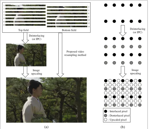
In consumer electronic devices such as HDTV systems, the VDFC technique is used to convert video sources into the kind of display resolution format shown in Figure 1. As shown in Figure 1b, deinterlacing doubles the vertical resolution of an interlaced image, while image upscaling resizes an image with arbitrary ratios. Therefore, image upscaling can be considered a generalized version of dein-terlacing. Moreover, the VDFC technique is generally based on either LFI or EDI approaches. However, LFI approaches tend to suffer from jagged artifacts along the
diagonal edges despite offering the competitive advan-tages of low complexity and arbitrary ratio interpolation. As large display devices with high resolution become more popular, the visible artifacts become more prominent. Although EDI approaches produce good performance in edge regions, they require high complexity in order to offer spatial coherence of the upscaled images. Also, these methods may require additional LFI methods for achiev-ing arbitrary ratio enlargement after performachiev-ing the EDI process. Therefore, an efficient VDFC technique, which offers a low computation load and provides high edge quality, is required.
3 5 7 9 11 13
2 4 6 8 10 12 14
Top field Bottom field
Deinterlacing (or IPC)
Image upscaling
Proposed video resampling method
Image upscaling Deinterlacing
(or IPC)
(a
)
(b
)
: Interlaced pixel : Denterlaced pixel : Upscaled pixel
Figure 1Display processing flow diagram.(a)Converting from incoming deinterlaced image to display format and(b)illustration of the position of the interpolated pixels.
order to solve this problem, a transient improvement (TI) technique is performed during the filtering process along the edge direction to improve the sharpness of the initially upscaled images. The JEC method is a core technique of the proposed video resampling system, and it can be used as a postprocessor for many LFI methods, such as cubic spline. This independent module can be applied to various applications with flexibility.
The organization of the rest of this paper is as follows: In Section 2, previous works on Lanczos interpolation and related issues are discussed. In Section 3, the proposed video resampling method is described in detail. First, the overall structure of the proposed method is explained. In Section 3.1, an image magnification step based on the Lanczos function is presented, and the proposed ringing
artifact reduction technique is described to improve inter-polation performance. Subsequently, the proposed JEC method is explained to improve the edge quality of the ini-tially interpolated images. In Section 4, the experimental results of various test images are presented, and compar-isons with other algorithms are made. Finally, conclusions are presented in Section 5.
2 Previous works on Lanczos interpolation
requirements of a hardware implementable interpolator. However, the truncated interpolation kernel produces severe ringing effects within interpolated images. There-fore, various windowing kernels such as Hann, Hamming, Cosine, Lanczos, Blackman, and Kaiser have been pro-posed to reduce these ringing effects. According to spec-tral analysis [12], these different windows display different spectral characteristics, and some tradeoffs occur when the window function is chosen. Thus, the choice of the windowing function is crucial, and it is very dependent on the selected applications. In Figure 2, we compare the sinc kernels truncated by various 6-tap windowing ker-nels. As shown in Figure 2a, each of the truncated sinc kernels has negative coefficients, which comes from the side lobes of a sinc function. These negative coefficients are used to produce steep and sharp edge transitions in the step edges and to recover the image details in the texture regions. Therefore, larger negative coefficients achieve better reconstruction performance in the edge regions. According to Figure 2b, the Lanczos windowing kernel has the most negative coefficients among the var-ious windowing kernels. Thus, the Lanczos windowing kernel is preferred in order to improve the reconstruction performance of the high-frequency components.
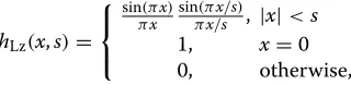
The impulse response of the Lanczos interpolator is the normalized sinc function windowed by the Lanczos win-dow, and the Lanczos window is the central lobe of a sinc function scaled to a certain extent. In one dimension, the Lanczos function can be obtained as
hLz(x,s)= ⎧ ⎨ ⎩
sin(πx) πx
sin(πx/s)
πx/s , |x|<s
1, x=0
0, otherwise,
(1)
where hLz(x,s) represents the Lanczos kernel and s is a positive integer (typically 2 or 3), which controls the
size of the Lanczos kernel. According to Figure 3, the Lanczos interpolator can achieve better reconstruction performance using wider windows (whensis set as 4, 8, or 12) since the interpolation kernels become similar to the ideal sinc function. However, if the window size increases, more side lobes of the ideal sinc function influence the interpolation kernels, and they cause unwanted artifacts such as ringing (or shooting) artifacts in flat regions, espe-cially when high-frequency edges exist within the range of the wide window. From the above discussion, it is clear that the side lobes of an interpolation filter can improve reconstruction performance in edge regions, but they can also degrade the image quality because of the ringing artifacts.
3 Proposed video resampling method with
jagged edge correction
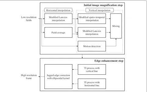
Figure 4 roughly illustrates the overall structure of the proposed resampling method. As illustrated in Figure 4, the proposed method requires two steps to perform video resampling: the initial image magnification step and the edge enhancement step. In the first step, the image magnification process for deinterlacing and upscal-ing is performed dimensionally by performupscal-ing one-dimensional interpolation processes in the horizontal and vertical directions separately. Interpolation kernels for directional interpolations are based on the Lanczos kernel with a ringing artifact reduction. Especially in the vertical interpolation process, temporal information is used and then the values of both modified spatio-temporal interpolation and modified Lanczos interpola-tion are mixed according to the mointerpola-tion detecinterpola-tion process. In the second step, the proposed JEC method is applied to the initially upscaled images to improve the edge quality of the images. During the JEC process, a TI technique is also used to improve the sharpness of the upscaled images.
(a)
(b)
(b)
(c)
(d)
(a)
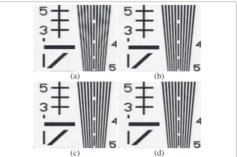
Figure 3Upscaled images obtained by varying the size of the Lanczos kernel.(a)Input image. Filter as(b)s=4,(c)s=8, and(d)s=12.
3.1 Initial image magnification step
3.1.1 Image magnification process with Lanczos function The goal of the proposed resampling method is to con-vert an interlaced field to a scaled progressive frame. In order to achieve this goal, the image magnification process performs one-dimensional interpolation first in the hori-zontal direction and then again in the vertical direction. Based on the Lanczos function, the missing pixel value at an arbitrary position(i,j)is reconstructed by
ˆ
fLzif(i+k,j+j,n)= a
l=−a+1
hLz(j−l,a)·fif
×(i+k,j+l,n), (2)
ˆ
fpf(i+i,j+j,n)=α· ˆfLzpf(i+i,j+j,n)
+(1−α)· ˆfSTpf(i+i,j+j,n), (3)
where the superscripts if and pf denote the interlaced image and the progressive image, respectively, and the subscripts Lz and ST represent the results of Lanczos interpolation and spatio-temporal interpolation, respec-tively. fif and fˆpf represent the input interlaced image
and the output upscaled progressive image, respectively.
ˆ
fLzif denotes the horizontally upscaled interlaced image, andfˆLzpfandfˆSTpf represent the upscaled progressive images obtained from Lanczos and spatio-temporal interpo-lations, respectively. (i,j) and n represent the spatial indices and the temporal index of the input interlaced image, respectively.arepresents the horizontal size of the Lanczos kernel.i andj (0 ≤ i,j < 1) represent the arbitrary positions to be interpolated in the vertical and horizontal directions, respectively. Since the pixels of the top and bottom fields are positioned alternately in the vertical direction, the relative vertical positions of the cur-rent, previous, and next fields are determined along the temporal index. Given the input interlaced imagefif,i andjare represented as
i=
i·srv− i·srv −(n%2)/2 ifn,(n±2)fields i·srv− i·srv if(n±1)fields j=j·srh− j·srh,
(4)
Modified Lanczos
Horizontal interpolation Vertical interpolation
Initial image magnification step
Edge enhancement step
Figure 4Overall block diagram of the proposed image resampling method.
real number.α of (3) is a weight to control the contribu-tion of two values,fˆLzpfandfˆSTpf. In the image magnification process, the horizontal scaling process is first performed using (2) and then the final results of the vertical interpo-lation are obtained from fusing Lanczos interpointerpo-lation and spatio-temporal interpolation according to the motion detection process.
In the vertical interpolation process of (3), fˆLzpf andfˆSTpf
mainly contribute to fˆpf in the motionless and motion areas, respectively. These values are calculated using pre-vious and next field information because the original pixel information at the missing position is obtained from the previous and next fields due to the inherent nature of the interlaced format. First, the ˆfLzpf value for the motionless areas is computed using the field average and a Lanczos kernel. That is,
where fˆFAif represents the results of the field average. b
represents the vertical size of the Lanczos kernel and δ denotes the Dirac delta function. Since the fˆFAif value is at the 0.5 position in the vertical direction, i for the sub-pixel position of the Lanczos kernel is modified:
i=2·i− 2·i. (7)
THF= ⎧ ⎪ ⎪ ⎨ ⎪ ⎪ ⎩
THFi−1·(0.5−i)+THFi·(0.5+i) if top fields andi≤0.5 THFi·(1.5−i)+THFi+1·(i−0.5) if top fields andi>0.5 THFi·(0.5+i)+THFi+1·(0.5−i) if bottom fields andi≤0.5 THFi+1·(i−0.5)+THFi·(1.5−i) if bottom fields andi>0.5
, (9)
where THF represents the high-frequency components of temporal information. Since the THF value is estimated only at the existing pixel position in the previous and next fields, a linear combination between the THFs at the neighboring pixels is used to obtain THF at an arbitrary position. According to characteristics of the top and bot-tom fields, the used THF is determined as shown in (9). THFiis defined as
THFi= c
k=−c
hTF(c+k)·
ˆ
fLzif(i+k,j+j,n−1)
+ ˆfLzif(i+k,j+j,n+1)
2, (10)
where
hTF=[−0.25 0.5 −0.25] . (11)
Figure 5 shows an example of obtaining the high-frequency component of temporal information.
For combining the results of Lanczos interpolation and spatio-temporal interpolation, the reliability terms of temporal information are used as weighting factors based on both motion detection and feathering artifacts. The motion detection process and the feathering artifact detection process are performed in each pixel position. For motion detection, the temporal difference,DTis com-puted through five fields in order to detect both normal and fast motions.DT is given by
DT= | ˆfLzif(i+k,j+j,n−1)− ˆfLzif(i+k,j+j,n+1)|
+ 1
k=0
l=0,2
| ˆfLzif(i+k,j+j,n−2+l)
− ˆfLzif(i+k,j+j,n+l)|
2. (12)
|x|returns the absolute value ofx. To detect the feathering artifacts, the vertical difference,DV is computed by using ˆ
fFAif.
DV =min{DV1,DV2,DV3}, (13)
n n+1
n-1 i-1 -0.25
0.5
-0.25 i
i+1
-0.25
0.5
-0.25
: : :
: Interlaced pixel : Deinterlacing
pixel position
(a)
(b)
n n+1
n-1 0
1
where
DV1= | ˆfLzif(i,j+j,n)− ˆfFAif (i,j+j,n)| DV2= | ˆfLzif(i,j+j,n)− ˆfFAif (i−1,j+j,n)| DV3= | ˆfLzif(i+1,j+j,n)− ˆfFAif(i+1,j+j,n)|,
(14)
The arbitration rules forαin (3) can be summarized as
α= min{DT+DV,τ1}
τ1 , (15)
where τ1 represents a predetermined constant for nor-malization. According to (12), ifDThas a large value, the current pixel can be considered a motion pixel. In these motion areas,DV has a large value generally because of the feathering artifacts. Thus, the final result is close to the result of spatio-temporal interpolation.
3.1.2 Ringing artifact reduction technique to improve interpolation performance
As discussed in Section 2, the side lobes of a Lanczos ker-nel can improve reconstruction performance along edge regions, but they often degrade image quality due to ringing artifacts. Moreover, although the temporal high pass filter of spatio-temporal interpolation can be use-ful to improve edge information, the resulting images generally suffer from shooting artifacts caused by over-shooting or underover-shooting. In our previous work [18], we introduced a kernel-based image upscaling method that handled the ringing artifact problem caused by using a wider window for the Lanczos kernel. An extension of these concepts is now presented in order to avoid ring-ing artifacts or shootring-ing artifacts. The proposed method is performed one-dimensionally after performing each one-dimensional interpolation process including Lanczos interpolation and spatio-temporal interpolation. Since ringing artifact reduction processes for Lanczos interpola-tion are similar to those discussed in [18], we only describe the ringing artifact reduction process for spatio-temporal interpolation in this section.
The proposed ringing artifact reduction method is com-posed of two steps: median filtering and arbitration. First, a median filter is applied to the result of spatio-temporal interpolation with the two nearest input data values. The result of median filtering is called the median spatio-temporal value in this paper. The median spatio-spatio-temporal value of the vertical direction is obtained as
ˆ
wherefˆmedSTpf andfˆarbiLzif represent the result of the median spatio-temporal value and the ringing artifact reduced result of the horizontal Lanczos interpolator, respectively, and med{x,y,z}represents a three-input median filter that
returns the median value ofx,y, andz. This median pro-cess is very efficient at removing ringing artifacts since it is particularly good for removing shot noise. However, this process often degrades image details by restricting the interpolated value within the values of its neighbor-ing pixels. This restriction prevents reconstructneighbor-ing the high-frequency components of an image.
In the second arbitration step, the two highly comple-mentary results are combined effectively in order to avoid ringing artifacts while reconstructing the high-frequency components. The arbitration process is performed using the results of (8) and (16) as follows:
ˆ
farbiSTpf (i+i,j+j,n)=β· ˆfSTpf(i+i,j+j,n)
+(1−β)· ˆfmedSTpf (i+i,j+j,n), (17)
where β (0 ≤ β ≤ 1) represents the weighting coef-ficient that controls the contribution of the two results. In the edge regions, β is determined near 1 to recon-struct the high-frequency components by adopting the spatio-temporal result. However, in regions with ringing artifacts, β decreases to remove the artifacts by adopt-ing the median spatio-temporal result. The arbitration weightβ is obtained with the difference values between the neighboring pixels as
β= min{DU,DD,τ2} τ2
, (18)
where τ2 represents a predetermined constant for nor-malization, and the differences (DU andDD) are obtained as
of both Lanczos interpolation and spatio-temporal inter-polation. Thus, the final result of the initial resampling step is obtained by
ˆ
fInitpf(i+i,j+j,n)=α· ˆfarbiLzpf (i+i,j+j,n) +(1−α)· ˆfarbiSTpf (i+i,j+j,n).
(20)
3.2 Edge enhancement step
Based on the LFI approach, the proposed method in Section 3.1 is used to resize images to fit the display for-mat. However, LFI approaches are likely to smooth image details during the resampling process, and they usually produce jagged edge artifacts in the diagonal edge regions. In this section, we propose an edge enhancement algo-rithm that corrects the jagged edge artifacts and improves the sharpness of the initially interpolated images. For convenience of notation, the initially upscaled image is represented as F(i,j) instead of fˆInitpf(i,j,n) as is used in (20).
3.2.1 Jagged edge correction with an ellipsoidal kernel In order to remove the jagged edge artifacts, an estima-tion of the edge direcestima-tion is important. In [18-20], it is assumed that the edge direction of interestF(i,j), whereF
represents the initially upscaled image, is piecewise con-stant and the gradient vectors within a small mask should on average be orthogonal to the edge direction. Therefore, the estimation of edge direction can be formulated as the task of finding a unit vectordto minimize the following cost function:
wheregv andgh represent derivatives in the vertical and horizontal directions, respectively.
A unique vectord that minimizes the cost function in (21) is a good estimate of an edge direction so that the JEC can be carried out in the direction ofd. However, this requires an additional technique such as singular value decomposition (SVD) to find a unique optimal solution
ford[19]. Therefore, instead of finding the optimal solu-tion, the cost function in (21) is used to estimate which vectors are closer to the edge direction in the proposed JEC method. Let d =[k l]T denote a vector pointing from the current pixel in (i,j) to the neighboring pixel in(i+k,j+l). Then, the similarity betweendand the edge direction is obtained by the cost function in (21) as follows:
As mentioned above, cost(d) decreases as the orienta-tion of d approaches the edge direction. However, ifd
is parallel to the gradient vector, cost(d)returns a large value. Using this characteristic, an adaptive smoothing kernel is obtained by adopting a Gaussian kernel as
(k,l)=exp
where (k,l) represents the coefficients of the adaptive smoothing kernel. The cost function in (23) represents an elliptic equation form, and it spread the Gaussian kernel along the local edge direction. Therefore, in this paper, this adaptive kernel is called an ellipsoidal kernel, which is similar to the steering kernel used in [21]. σ in (24) controls the scale of the kernel, and it is determined as
σ =ν·max(c00,c11), (25)
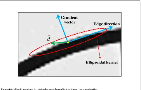
where ν represents a predetermined smoothing param-eter. In Figure 6, an example of an ellipsoidal kernel is illustrated with the gradient vector, the edge direction, and an arbitrary vectord. As shown in (24) and Figure 6, the ellipsoidal kernel assigns large weights along the edge direction. Therefore, pixels in the similar edge directions are smoothed by the ellipsoidal kernel, and as a result, jagged edge artifacts are corrected.
Gradient
vector
Edge direction
Ellipsoidal kernel
d
Figure 6An ellipsoid kernel and its relation between the gradient vector and the edge direction.
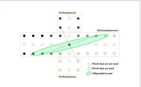
as shown in Figure 7. With the remaining pixels, the pro-posed method is performed in the horizontal and vertical directions. First, the horizontal process is performed as
Zhor=
L
l=0,l=−L
(−1,l)+(1,−l)=2·
L
l=0,l=−L
(−1,l)
FJc-hor(i,j)=
L
l=0,l=−L
(−1,l)·F(i−1,j+l)+(1,−l)·
×F(i+1,j−l)
=2·
L
l=0,l=−L
(−1,l)·Fhor(i,j+l),
(26)
where F and FJc-hor represent the initially interpolated image and the weighted sum of the horizontal process, respectively.Zhoris used for normalization andFhor(i,j+l) is defined as
Fhor(i,j+l)=
F(i−1,j+l)+F(i+1,j−l)
2 . (27)
In (26), (1,−l) is the same as (−1,l) since an ellip-soidal kernel is point symmetric with respect to the middle point. In the same way, the vertical process is performed as
Zver=2· K
|k|>1,k=−K
(−k,−1),
FJc-ver(i,j)=2· K
|k|>1,k=−K
(−k,−1)·Fver(i−k,j),
(28)
whereFJc-verrepresents the weighted sum in the vertical direction.Zver is used for normalization andFver(i−k,j) is defined as
Fver(i−k,j)=
F(i−k,j−1)+F(i+k,j+1)
2 . (29)
From (26) and (28), the final JEC result is obtained as
FJc(i,j)=
F(i,j)+FJc-hor(i,j)+FJc-ver(i,j) 1+Zhor+Zver
. (30)
Horizontal process Vertical process
Vertical process
: Pixels that are not used
: Pixels that are used
: Ellipsoidal kernel
Figure 7The proposed JEC process with an ellipsoidal kernel.
was used to reduce these stair-like artifacts by smoothing them along the local edge direction. However, since the ellipsoidal kernel is a kind of low pass filter, some image details are smoothed by the kernel during the filtering process. Therefore, in this paper, a TI technique is simul-taneously performed with the filtering process in order to improve the sharpness of the initially interpolated images. From the viewpoint of enhancing the sharpness of an image, the basic idea of the TI methods may seem sim-ilar to that of general sharpening methods. However, TI methods are more specialized in terms of improving the slow transitions of blurred edges since these methods fun-damentally prevent overshooting and undershooting. In order to improve the slow transition with general ening methods, we have to increase the amount of sharp-ening. However, an excessive amount of sharpening tends to degrade image quality because it produces severe over-shooting and underover-shooting. These factors often produce white and black bands along the contrasting edges, which appear unpleasant. However, TI algorithms can produce steep and natural edge transitions without undershooting and overshooting. In image upscaling applications, a lot of edges show poor transitions so the TI technique can be used efficiently to improve the sharpness of the upscaled images. In Figure 8, the behavior of the TI algorithm is illustrated briefly.
TI methods generally consist of two steps [22-24]. In the first step, a high-frequency boost filter is adopted as a pre-filter to enhance the slow transition of blurred edges. That is, a correction signal is added to the blurred signal to reconstruct the original high-frequency component. The above description can be written as the following equation:
XHB=Xin+hHF∗Xin=hHB∗Xin, (31)
whereXinandXHBrepresent the input signal and the fil-tered result, respectively. hHF and hHB represent a high pass filter and a high-frequency boost filter, respectively. For example, the second-order derivative operator has been used ashHFin several conventional methods. In the second step, the processed signal is limited to the proper range to prevent overshooting and undershooting:
XTI(i,j) =TI
XHB(i,j),τmax,τmin
=
⎧ ⎨ ⎩
τmax, if XHB(i,j) > τmax τmin, if XHB(i,j) < τmin
XHB(i,j), otherwise
. (32)
Local maximum
Local minimum
: blurred edge
: after TI
Figure 8Transient improvement method using local maximum and local minimum values.
Section 3.2.1. The TI process is performed in the vertical and horizontal directions. Since the vertical and horizon-tal filtering processes are exactly the same, we will only describe the horizontal process in this paper.
In (26) and (27), Fhor(i,j+ l) is used for the filtering process, and it is obtained by averaging F(i − 1,j+ l) and F(i+ 1,j− l). However, this direct average causes blurring effects during the filtering process when the two values are quite different. Therefore, the TI technique is applied toFhor(i,j+l)to reduce the blurring effects. Let
FTI-hor(i,j+l) be the result of the TI process, which is used instead ofFhor(i,j+l). Then, (26) is changed to the following equation:
Zhor=2·
L
l=0,l=−L
(−1,l)
FJc-hor(i,j)=2·
L
l=0,l=−L
(−1,l)·FTI-hor(i,j+l),
(33)
a
b1
c2 c1
)
,
,
25
.
0
25
.
0
5
.
0
5
.
0
5
.
0
(
a
b
1b
2c
1c
2τ
maxτ
minTI
TIout
=
+
+
−
−
b2
− −
.25 0 0 0 0 5 . 0
0 0 5 . 0 0 0
5 . 0 0 0 0 25 . 0
−
−
5 . 0 0 0 0 25 . 0
0 0 5 . 0 0 0
25 . 0 0 0 0 5 . 0
(a)
(b)
(c)
Filter coefficient #1 Filter coefficient #2
Figure 10The effect of the proposed TI process performed in two directions.(a)Upscaled image produced by the Lanczos interpolator with the ringing reduction and the results of the TI process when(b)l=2 and(c)l= −2.
(b)
(c)
(d)
(a)
Figure 11Upscaled images obtained by varying the size of the Lanczos kernel.(a)Input image. Horizontal kernel size(b)a=4,
whereFTI-hor(i,j+l)is obtained as frequency boost filtering. It is obtained by adding the high-frequency components toFhor(i,j+l)as ingb1andb2in the direction of the green arrow. High pass
filtering is applied to the pixels [a,c1,c2] in the opposite direction toFhor(i,j+l)(along the dotted purple arrow). We supposed the direction of the green arrow to be sim-ilar to the real edge direction. Then,a,c1, andc2 in the opposite direction to the green arrow form a contrasting edge, and the high-frequency components are extracted from this edge. That is, the high-frequency components obtained from pixels across an edge (a,c1, andc2) are used to restore the blurred edges of an initially interpolated image. After the filtering process, the filtered value is lim-ited to the proper range betweenτmaxandτminto prevent artifacts caused by overshooting and undershooting:
Fmin(l)represent the local maximum and local minimum values within the range of [−|l|,|l|]. The local extremums are searched on the middle line among the three lines illustrated in Figure 9. In general, the middle line usually
(a)
crosses over the edges on(i,j)so that it contains both the maximum and minimum pixel values within a local win-dow. From (34) to (36), we obtainFTI-hor(i,j+l), which provides sharper images thanFhor(i,j+l).
In Figure 10, we present two examples of the proposed TI process when l = 2 and l = −2. As shown in Figure 10b, jagged edge artifacts are reduced along the edges at 0° to 45° angles (blue circled) when l = 2. However, when l = −2, the jagged edge artifacts are
reduced along the edges at 135° to 180° angles (red cir-cled) in Figure 10c. Even though the edges at 135° to 180° angles in Figure 10b and the edges at 0° to 45° angles in Figure 10c are degraded by the TI process, the degraded results are excluded by the ellipsoidal kernel. In the pro-posed method, the ellipsoidal kernel assigns large weights along the estimated edge direction. Therefore, thel = 2 results in Figure 10b dominate the final results along the edges at 0° to 45° angles, and the l = −2 results in
(a)
(d)
(g)
(f) (e)
(c)
(b)
Figure 13Results of conventional deinterlacing methods and the proposed method.(a)CS,(b)Lanczos,(c)NEDD,(d)LSMD,(e)STCAD,
Table 1 PSNRs (dB) of various deinterlacing methods including the proposed method
LFI EDI Combination
CS Lanczos NEDD LSMD STCAD MAVTF Proposed method
Bus 28.44 28.43 28.23 28.05 28.24 28.78 28.82
Coastguard 29.08 29.31 29.31 29.29 31.38 31.23 31.77
Container 28.96 29.08 29.00 28.84 35.55 35.45 35.71
Foreman 34.31 34.50 34.60 35.00 36.43 36.78 37.51
Hall monitor 32.10 32.20 32.07 31.65 38.25 37.75 38.43
Mom daughter 33.38 33.67 33.76 33.69 38.14 38.30 38.48
Silent 34.13 34.38 34.47 34.59 39.93 40.33 40.43
Rodmap 28.49 28.09 27.51 28.36 30.25 29.85 30.47
Washdc 32.49 32.23 31.80 31.82 38.14 37.70 38.48
Mobile 32.54 32.84 32.92 32.89 34.53 34.90 34.41
Stockholm 32.55 32.88 32.99 32.93 33.83 33.07 33.85
Shields 30.99 31.25 31.31 31.21 30.92 30.70 31.17
Average 31.45 31.57 31.49 31.52 34.63 34.57 34.96
The highest PSNR values are set in italics.
Figure 10c dominate the final results along the edges at 135° to 180° angles, respectively.
For the vertical process,FTI-ver(i−k,j)is used instead of
Fver(i−k,j), and it is obtained by
FTI-ver(i−k,j)=TI
FHB-ver(i−k,j),τmax,τmin
, (37)
and the vertical JEC process is performed as
Zver=2· K
|k|>1,k=−K
(−k,−1),
FJc-ver(i,j)=2· K
|k|>1,k=−K
(−k,−1)·FTI-ver(i−k,j).
(38)
The final JEC result is obtained by (30).
Table 2 SSIMs of various deinterlacing methods including the proposed method
LFI EDI Combination
CS Lanczos NEDD LSMD STCAD MAVTF Proposed method
Bus 0.912 0.913 0.908 0.904 0.910 0.915 0.916
Coastguard 0.831 0.838 0.839 0.835 0.918 0.916 0.914
Container 0.911 0.916 0.917 0.912 0.984 0.982 0.985
Foreman 0.940 0.944 0.947 0.948 0.958 0.960 0.967
Hall monitor 0.967 0.968 0.968 0.962 0.978 0.975 0.980
Mom daughter 0.946 0.949 0.952 0.950 0.969 0.972 0.973
Silent 0.927 0.931 0.932 0.933 0.972 0.987 0.985
Rodmap 0.938 0.936 0.931 0.940 0.962 0.964 0.967
Washdc 0.955 0.950 0.952 0.951 0.988 0.981 0.988
Mobile 0.908 0.916 0.918 0.921 0.932 0.936 0.937
Stockholm 0.890 0.898 0.901 0.900 0.913 0.915 0.915
Shields 0.913 0.918 0.920 0.918 0.921 0.916 0.921
Average 0.919 0.923 0.923 0.922 0.950 0.951 0.954
4 Experimental results
The performance of the proposed method was tested with well-known common intermediate format (CIF), SD, and HD video sequences. We converted the pro-gressive sequences into an interlaced format or down-sampled them according to experimental purposes. For performance comparisons, three groups of conventional deinterlacing methods were implemented: LFI approaches including cubic spline (CS) [11] and Lanczos, EDI approaches including new edge dependent deinterlacing (NEDD) [13] and local surface model-based deinterlac-ing (LSMD) [14], and a combination of both LFI and EDI approaches including spatial-temporal content-adaptive deinterlacing (STCAD) [3] and motion adaptive vertical temporal filtering (MAVFT) [4]. Two groups of image upscaling methods were implemented: LFI approaches including CS [11], EDI approaches including new edge-directed interpolation (NEDI) [15] and soft-decision adaptive interpolation (SAI) [17]. In the experiments, the
interpolated positions of deinterlacing and upscaling were adaptively adjusted for the CS and Lanczos, respectively. Lanczos represents Lanczos interpolation without apply-ing the proposed rapply-ingapply-ing reduction method.
The peak signal-to-noise ratio (PSNR) and the struc-tural similarity (SSIM) [25] of the luminance channel were used for quantitative measurement. The PSNR is defined as PSNR = 10log10(2552/MSE), where MSE represents the mean squared error between the original and the reconstructed images. The SSIM compared local patterns of pixel intensities that were normalized for luminance and contrast. Thus, the SSIM was used to gauge the visual quality of images more closely to the human visual system. The SSIM index is represented by
SSIM(om,rm)=
(2μoμr+C1)(2σor+C2) (μ2
o+μ2r +C1)(σo2+σr2+C2) ,
(39)
(a)
(d)
(e)
(c)
(b)
Table 3 PSNRs (dB) of various VDFC methods including the proposed method
LFI EDI Combination
CS Lanczos NEDI SAI Proposed method
Bus 21.11 21.35 20.84 21.22 21.43
Coastguard 24.18 24.36 24.05 24.27 25.40
Container 24.01 24.31 23.58 24.13 24.96
Foreman 30.52 30.96 30.43 30.77 31.33
Hall monitor 25.86 26.00 25.26 25.76 26.34
Mom daughter 29.14 29.62 28.82 29.25 30.11
Silent 29.77 30.50 29.65 29.98 30.32
Rodmap 20.58 20.83 20.38 20.65 21.25
Washdc 24.59 24.77 23.75 24.37 24.31
Mobile 27.54 27.81 27.02 27.57 27.88
Stockholm 27.79 28.06 27.42 27.85 28.22
Shields 25.45 25.82 25.28 25.62 25.93
Average 25.87 26.19 25.54 25.95 26.45
Resampled images of CS, Lanczos, NEDI, and SAI were obtained after performing the STCAD. The highest PSNR values are set in italics.
where o andr represent the original and reconstructed images, respectively. om andrm are the image contents at themth windows of the image.μandσ represent the mean and standard deviation of each pixel over a 11×11 pixel Gaussian window, respectively. σor represents the covariance value of each pixel over a 11×11 pixel Gaussian window on the original and reconstructed images.C1 and
C2 are constant values to increase stability:C1 = 6.5025 and C2 = 58.5225 for 8-bit images. In order to evalu-ate the overal image quality, a mean structural similarity (MSSIM) was employed.
MSSIM(o,r)= 1 M
M
m=1
SSIM(om,rm), (40)
whereMrepresents the number of local windows of the image. The MSSIM ranged from 0 to 1. Therefore, a higher MSSIM value close to 1 meant that a given image was reconstructed with reduced degradation of structural information.
There are several parameters in the proposed method. Most of these parameters were set empirically and tested with various images to obtain the best results.ain (2) and
Table 4 SSIMs of various VDFC methods including the proposed method
LFI EDI Combination
CS Lanczos NEDI SAI Proposed method
Bus 0.648 0.653 0.643 0.650 0.651
Coastguard 0.584 0.588 0.582 0.585 0.641
Container 0.773 0.778 0.769 0.775 0.824
Foreman 0.878 0.881 0.872 0.879 0.896
Hall monitor 0.860 0.864 0.843 0.862 0.877
Mom daughter 0.880 0.883 0.874 0.881 0.897
Silent 0.831 0.834 0.825 0.832 0.848
Rodmap 0.768 0.773 0.765 0.771 0.776
Washdc 0.803 0.809 0.794 0.805 0.808
Mobile 0.779 0.786 0.778 0.787 0.792
Stockholm 0.754 0.761 0.751 0.759 0.761
Shields 0.722 0.728 0.720 0.726 0.733
Average 0.773 0.778 0.768 0.776 0.792
bin (5) represent the sizes of the interpolation filters in the horizontal and vertical directions, respectively. Since the side lobes of a Lanczos kernel improved reconstruction performance along the edge regions, the used kernel size
severely impacted the performance of the reconstructed image. In Figure 11, we presented the upscaled images obtained by varying the size of the Lanczos interpola-tion kernel to analyze the effect of the kernel size on the
(a)
(d)
(f)
(e)
(c)
(b)
(h)
(g)
Figure 15Results of the proposed JEC method after the deinterlacing process.(a)CS,(b)JEC after CS,(c)Lanczos,(d)JEC after Lanczos,
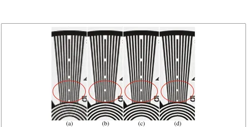
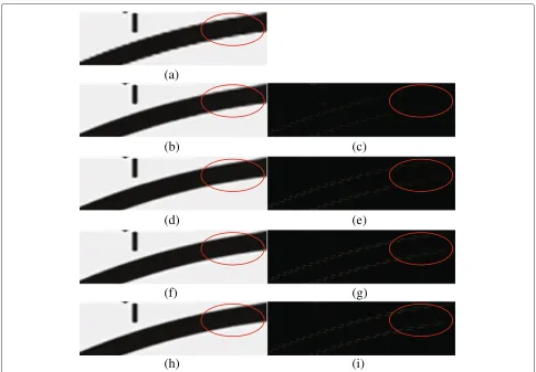
image quality. Figure 11a presents the input image with the vertically patterned edges. In Figure 11b,c,d, it was upscaled by a factor of 2, and different kernel sizes were used for each result. The horizontal kernel sizes were set as 4, 8, and 12 in Figure 11b,c,d, respectively. As shown in the figures, the high-frequency components were recon-structed well as the kernel size increased. In our obser-vations, there was little improvement when the size was larger than 8. Therefore, we set the size as 8, as a com-promise between performance and hardware complexity. In the experiments, we used a smaller interpolation fil-ter in the vertical direction because of the line memory restriction of the hardware structure. Thus,aandbwere set as a = 8 and b = 6, respectively. Also, τ1 in (15) andτ2in (18) represent the predetermined constants for normalization. For 8-bit images,τ1was set as 96 for the mixing process of vertical interpolation, andτ2 was set as 64 for the ringing artifact reduction process. Gener-ally, the window size used for the JEC process is the most important factor in determining performance, and there-fore, a sufficient window size was required to reduce the jagged edge artifacts along the nearly horizontal or ver-tical edges. In Figure 12, we presented the jagged edge corrected images obtained by varying the window size of the JEC process to analyze the effect of the window size on the image quality. Figure 12a presents the input image
with the nearly horizontal edge, which was degraded by the jagged edge artifacts. In Figure 12b,d,f,h, it was cor-rected by the JEC process, and different window sizes were used for each result. The horizontal window size were set as 5, 7, 9, and 11, respectively. As shown in the figures, the jagged edge artifacts were reduced substantially by the JEC process. In order to compare the performance of the JEC process with various window sizes, the difference images between the input image and the reconstruction images are presented in Figure 12c,e,g,i, and the difference image presents the jagged edge artifacts corrected by the JEC process. As shown in the figures, the jagged edge artifacts were reduced well as the window size increased. In our observation, there was little improvement when the size was larger than 7. Therefore,L in (26) and (33) was set as 7 for the horizontal process. However, the vertical win-dow sizeKin (28) and (38) was set as 3 to reduce the line memory required for hardware implementation. We used the same parameter values for all the test images.
In Figure 13, the performance of the proposed method was evaluated for the deinterlacing process. For this experiment, test video sequences were converted into an interlaced format and then the interlaced sequences were deinterlaced again with conventional deinterlacing methods. Figure 13a,b,c,d,e,f,g represents the deinter-laced results of CS, Lanczos, NEDD, LSMD, STCAD,
(a)
(d)
(c)
(b)
Table 5 PSNRs (dB) of various deinterlacing methods with and without the proposed JEC method
CS Lanczos STCAD MAVTF
Initial JEC Initial JEC Initial JEC Initial JEC
BUS 28.44 28.44 28.43 28.44 28.24 28.26 28.78 28.87
Coastguard 29.08 29.15 29.31 29.35 31.38 31.79 31.23 31.67
Container 28.96 29.16 29.08 29.26 35.55 35.80 35.45 35.73
Foreman 34.31 35.46 34.50 36.07 36.43 37.47 36.78 37.88
Hall monitor 32.10 32.22 32.20 32.34 38.25 38.34 37.75 38.31
Mom daughter 33.38 33.39 33.67 33.80 38.14 38.08 38.30 38.46
Silent 34.13 34.26 34.38 34.58 39.93 39.21 40.33 40.76
Rodmap 28.49 28.44 28.09 28.49 30.25 30.50 29.85 30.22
Washdc 32.49 32.39 32.23 32.24 38.14 38.37 37.70 37.43
Mobile 32.54 32.75 32.84 33.11 34.53 34.61 34.90 35.08
Stockholm 32.55 32.66 32.88 32.97 33.83 33.83 33.07 33.29
Shields 30.99 30.96 31.25 31.33 30.92 31.77 30.70 30.78
Average 31.45 31.60 31.57 31.83 34.63 34.84 34.57 34.87
The JEC algorithm was applied to the deinterlaced image obtained by the initial deinterlacing methods. The higher PSNR values are set in italics.
MAVTF, and the proposed method, respectively. As shown in Figure 13, the existing methods produced jagged edge artifacts along the diagonal edges in red circled regions, but the proposed method provided satisfactory outputs without jagged edge artifacts. Tables 1 and 2 show the PSNRs and the MSSIMs of various deinterlac-ing methods, respectively. As described in Table 1, the proposed method recorded higher PSNR values than con-ventional deinterlacing methods in the majority of the test sequences. According to Table 2, the proposed method recorded higher MSSIM values than conventional dein-terlacing methods in the majority of the test sequences. These experimental results demonstrate that the pro-posed method can be used for deinterlacing process to improve image quality.
In Figure 14, the performance of the proposed method was evaluated for the VDFC process. For this experiment, the test video sequences were downsampled by a factor of 2 and then these sequences were converted into an interlaced format. Again, the downsampled and interlaced sequences were deinterlaced with conventional deinter-lacing methods and then progressive sequences were upsampled with conventional image upscaling methods. The STCAD was used to convert the interlaced format into a progressive format because the STCAD achieved high PSNR and SSIM values among the conventional deinterlacing methods (as shown in Tables 1 and 2). Figure 14a,b,c,d represents the results obtained from CS, Lanczos, NEDI, and SAI after performing STCAD. As shown in the red circled regions of Figure 14, LFI-based image upsampling methods in Figure 14a,b suffered from jagged edge artifacts along the diagonal edges, and EDI-based image upsampling methods in Figure 14c,d
provided fine results along the diagonal edges. How-ever, NEDI and SAI introduced some artifacts in the neighborhood regions of the character regions due to an incorrect estimation of covariance. However, the pro-posed method produced high-quality images by connect-ing discontinuous edges and reduced the jagged edge artifacts substantially. Tables 3 and 4 present the PSNRs and the MSSIMs of various VDFC methods, respectively. As described in Table 3, the proposed method recorded higher PSNR values than conventional VDFC methods in
Table 6 PSNRs (dB) of various image upscaling methods with and without the proposed JEC method
CS Lanczos
Initial JEC Initial JEC
Bus 25.85 25.89 26.21 26.32
Coastguard 28.42 28.42 28.87 28.90
Container 26.97 27.06 27.33 27.49
Foreman 33.60 34.03 34.14 35.53
Hall monitor 28.63 28.68 29.15 28.28
Mom daughter 32.22 32.13 32.45 32.75
Silent 31.93 31.90 32.40 32.61
Rodmap 27.37 27.01 27.22 27.76
Washdc 28.46 28.46 28.55 28.71
Mobile 29.86 29.96 30.31 30.56
Stockholm 31.07 31.11 31.57 31.66
Shields 29.15 29.12 29.80 29.92
Average 29.47 29.48 29.83 30.12
Table 7 SSIMs of various deinterlacing methods with and without the proposed JEC method
CS Lanczos STCAD MAVTF
Initial JEC Initial JEC Initial JEC Initial JEC
Bus 0.912 0.912 0.913 0.913 0.910 0.912 0.915 0.917
Coastguard 0.831 0.828 0.838 0.833 0.918 0.923 0.916 0.919
Container 0.911 0.913 0.916 0.917 0.984 0.985 0.982 0.984
Foreman 0.940 0.946 0.944 0.951 0.958 0.961 0.960 0.964
Hall monitor 0.967 0.968 0.968 0.969 0.978 0.978 0.975 0.978
Mom daughter 0.946 0.947 0.949 0.950 0.969 0.967 0.972 0.971
Silent 0.927 0.929 0.931 0.933 0.972 0.970 0.987 0.988
Rodmap 0.938 0.939 0.936 0.940 0.962 0.964 0.964 0.965
Washdc 0.955 0.955 0.950 0.955 0.988 0.989 0.981 0.983
Mobile 0.908 0.912 0.916 0.919 0.932 0.934 0.936 0.938
Stockholm 0.890 0.892 0.898 0.898 0.913 0.911 0.915 0.915
Shields 0.913 0.913 0.918 0.918 0.921 0.922 0.916 0.919
Average 0.919 0.921 0.923 0.924 0.950 0.951 0.951 0.953
The JEC algorithm was applied to the deinterlaced image obtained by the initial deinterlacing methods. The higher SSIM values are set in italics.
the majority of the test sequences. According to Table 4, the proposed method recorded higher MSSIM values than conventional VDFC methods. From Tables 3 and 4, it can be verified that the proposed method outperformed the conventional approaches in terms of numerical values.
The performance of the proposed JEC method was also evaluated. We applied the proposed method to the dein-terlaced images and the upscaled images. Figure 15a,c,e,g represents the deinterlaced results of CS, Lanczos, STCAD, and MAVTF, respectively. Using each figure as an input image, the proposed JEC method was performed to obtain the results in Figure 15b,d,f,h. Figure 16a,c represents the upscaled results of the CS and Lanczos, respectively. Using each figure as an input image, the proposed method obtained the results in Figure 16b,d. As shown in Figures 15 and 16, the jagged edge arti-facts were reduced substantially by the proposed method. Tables 5 and 6 present the PSNRs of various deinter-lacing methods and image upscaling methods, respec-tively. As described in Table 5, the proposed method improved the PSNR of CS, Lanczos, STCAD, and MAVTF by 0.15, 0.26, 0.21, and 0.3, respectively. As described in Tables 6, the proposed method improved the PSNR of CS and Lanczos by 0.01 and 0.29, respectively. In Tables 7 and 8, the MSSIMs of various deinterlacing methods and image upscaling methods are compared. As described in Table 7, the proposed method improved the MSSIM of CS, Lanczos, STCAD, and MAVTF by 0.002, 0.001, 0.001, and 0.002, respectively. According to Table 8, the pro-posed method improved the MSSIM of CS and Lanczos by 0.001 and 0.003, respectively. These experimental results demonstrate that the proposed JEC method can be used
as a postprocessor for various deinterlacing methods and image upscaling methods in order to improve the image quality.
To show the computational requirements, the aver-age run times of various imaver-age formats were calculated (as shown in Table 9). For this experiment, we used a PC equipped with an Intel Core2 Quad Q8200 CPU. Especially, the resampled images of CS, Lanczos, NEDI, and SAI were obtained after performing the SAVTF. Thus, the processing time of SAVTF was added to
Table 8 SSIMs of various image upscaling methods with and without the proposed JEC method
CS Lanczos
Initial JEC Initial JEC
Bus 0.85 0.85 0.856 0.857
Coastguard 0.793 0.792 0.802 0.802
Container 0.872 0.873 0.882 0.884
Foreman 0.923 0.926 0.930 0.938
Hall monitor 0.918 0.919 0.927 0.929
Mom daughter 0.930 0.930 0.933 0.937
Silent 0.887 0.888 0.892 0.895
Rodmap 0.924 0.921 0.922 0.929
Washdc 0.904 0.905 0.907 0.911
Mobile 0.842 0.845 0.854 0.859
Stockholm 0.844 0.845 0.856 0.857
Shields 0.878 0.878 0.885 0.888
Average 0.880 0.881 0.887 0.890
Table 9 CPU times of various VDFC methods including the proposed method for various image formats
Image format CS Lanczos NEDI SAI Proposed method
CPU CIF (352×288) 0.049 0.013 0.898 4.344 0.833
time (s) SD (720×486) 0.198 0.047 2.428 16.662 3.031
HD (1, 280×720) 0.443 0.115 8.498 39.433 7.578
Full HD (1, 920×1, 080) 1.005 0.259 19.829 86.689 16.812
Resampled images of CS, Lanczos, NEDI, and SAI were obtained after performing the STCAD.
the total processing times of the conventional meth-ods. As described in Table 9, the processing times increased depending on the resolution of the image for-mat. Although EDI-based methods needed more time than LFI-based methods due to requiring many oper-ations to estimate the edge direction, the EDI-based methods provided high-quality results and the LFI-based methods suffered from jagged edge artifacts in the diag-onal edge regions. According to Table 9, the process-ing time of the proposed method was similar to that of NEDI. Thus, the proposed method and the NEDI method have similar complexity levels. However, the proposed method provided better objective and subjective perfor-mance than the other methods. Furthermore, the JEC process of the proposed method can be used as a post-processor for performance improvement of many linear filtering interpolation methods. Thus, either the total pro-posed method or the JEC method can be selectively used according to the applications.
5 Conclusions
In this paper, we have proposed a flexible video resam-pling method with the advantages of both the LFI and EDI methods: the capabilities of converting image for-mats, resizing images for arbitrary ratios and improv-ing edge quality. The proposed method converted input interlaced sequences into upscaled progressive sequences simultaneously and improved the image quality of resam-pled images by correcting various interpolation artifacts, such as ringing, blurring, and jagged edge artifacts. In order to reduce the ringing artifacts, the proposed ringing reduction method was combined with Lanczos interpo-lation and spatio-temporal interpointerpo-lation. Also, the pro-posed JEC method was applied to initially upscaled images to correct jagged edge artifacts and to improve the sharp-ness of the images. Especially, this JEC postprocessor can be very useful for various image resampling applications since it is often used in combination with other common LFI techniques. The proposed algorithm was applied to various test images to verify the performance. Simula-tion results show that the proposed method outperformed conventional methods both visually and numerically.
Competing interests
The authors declare that they have no competing interests.
Acknowledgements
This work was supported by the National Research Foundation of Korea (NRF) grant funded by the Korea government (MSIP) (No. 2012R1A2A4A01003732).
Received: 31 July 2013 Accepted: 2 December 2013 Published: 20 December 2013
References
1. G de Haan, Large-video-display-format conversion. J. Soc. Inf. Display8(1), 79–87 (2000)
2. G de Haan, EB Bellers, Deinterlacing - an overview. Proc. IEEE86(9), 1839–1857 (1998)
3. GG Lee, H-Y Lin, M-J Wang, R-L Lai, CW Jhuo, B-H Chen, Spatial-temporal content-adaptive deinterlacing algorithm. IET Image Process.2(6), 323–336 (2008)
4. K Lee, J Lee, C Lee, Deinterlacing with motion adaptive vertical temporal filtering. IEEE Trans. Consum. Electron.55(2), 636–643 (2009)
5. Y-L Chang, S-F Lin, C-Y Chen, L-G Chen, Video deinterlacing by adaptive 4-field global/local motion compensated approach. IEEE Trans. Circuits Syst. Video Technol.15(12), 1569–1582 (2005)
6. Y-R Chen, S-C Tai, True motion compensated deinterlacing algorithm. IEEE Trans. Circuits Syst. Video Technol.19(10), 1489–1498 (2009) 7. Q Huang, D Zhao, S Ma, W Gao, H Sun, Deinterlacing using hierarchical
motion analysis. IEEE Trans. Circuits Syst. Video Technol.20(5), 673–686 (2010)
8. CE Shannon, Communication in the presence of noise. Proc. I.R.E.MI-2, 31–39 (1983)
9. TM Lehmann, C Gönner, Survey: interpolation methods in medical image processing. IEEE Trans. Med. Imaging18(11), 1049–1075 (1999) 10. RG Keys, Cubic convolution interpolation for digital image processing.
IEEE Trans. Acoustics, Speech Signal Process.29(6), 1153–1160 (1981) 11. HS Hou, HC Andrews, Cubic splines for image interpolation and digital
filtering. IEEE Trans. Acoustics, Speech Signal Process.508(6), 517 (1978) 12. T TheuBl, H Hauser, ME Gröller, Mastering windows: improving
reconstruction, inProceedings of the 2000 IEEE Symposium on Volume Visualization(Salt Lake City, 9–10 Oct 2000), pp. 101–108
13. MK Park, MG Kang, K Nam, SG Oh, New edge dependent deinterlacing algorithm based on horizontal edge pattern. IEEE Trans. Consum. Electron.49(4), 1508–1512 (2003)
14. S-J Park, J Jeong, Local surface model-based deinterlacing algorithm. Opt. Eng.50(1), 017004-1–017004-10 (2011)
15. X Li, New edge-directed interpolation. IEEE Trans. Image Process.10(10), 1521–1527 (2001)
16. WS Tam, CW Kok, WC Siu, Modified edge-directed interpolation for images. J. Electron. Imaging19(1), 013011 (2010)
17. X Zhang, X Wu, Image interpolation by adaptive 2-D autoregressive modeling and soft-decision estimation. IEEE Trans. Image Process.17(6), 887–896 (2008)
18. CH Park, J Chang, MG Kang, Kernel-based image upscaling method with shooting artifact reduction. Proc. SPIE 8655 Image Processing: Algorithms and Systems XI (2013). doi: 10.1117/12.2003326
19. X Feng, P Milanfar, Multiscale principal components analysis for image local orientation estimation, inConference record of the 36th Asilomar Conference on Signals, Systems and Computers(Pacific Grove, 3–6 Nov 2002), pp. 478–482
21. H Takeda, S Frsiu, P Milanfar, Kernel regression for image processing and reconstruction. IEEE Trans. Image Process.16(2), 349–366 (2007) 22. P Lin, YT Kim, An adaptive color transient improvement algorithm.
IEEE Trans. Consum. Electron.49(4), 1326–1329 (2003) 23. K Ohara, Digital color transient improvement. U.S. Patent,
5,920,357, 6 July 1999
24. J Chang, GS Shin, JH Park, MG Kang, Color transient improvement for signals with a bandlimited chrominance component. Opt. Eng.46(2), 027002.1–027002.11 (2007)
25. Z Wang, AC Bovik, HR Sheikh, EP Simoncelli, Image quality assessment: from error visibility structural similarity. IEEE Trans. Image Process.13(4), 600–612 (2004)
doi:10.1186/1687-6180-2013-188
Cite this article as:Yooet al.:Video resampling algorithm for simultaneous deinterlacing and image upscaling with reduced jagged edge artifacts.
EURASIP Journal on Advances in Signal Processing20132013:188.
Submit your manuscript to a
journal and benefi t from:
7Convenient online submission
7Rigorous peer review
7Immediate publication on acceptance
7Open access: articles freely available online
7High visibility within the fi eld
7Retaining the copyright to your article