Generalization of a 3-D Acoustic Resonator
Model for the Simulation of Spherical
Enclosures
Davide Rocchesso
Università di Verona, Dipartimento Scientifico e Tecnologico, Strada Le Grazie 15, I-37134 Verona, Italy Email: [email protected]
Pierre Dutilleux
Zentrum für Kunst und Medientechnologie (ZKM), Institute for Music and Acoustics, Lorenzstrasse 19, D-76135 Karlsruhe, Germany Email: [email protected]
Received 20 April 2000 and in revised form 9 October 2000
A rectangular enclosure has such an even distribution of resonances that it can be accurately and efficiently modelled using a feedback delay network. Conversely, a nonrectangular shape such as a sphere has a distribution of resonances that challenges the construction of an efficient model. This work proposes an extension of the already known feedback delay network structure to model the resonant properties of a sphere. A specific frequency distribution of resonances can be approximated, up to a certain frequency, by inserting an allpass filter of moderate order after each delay line of a feedback delay network. The structure used for rectangular boxes is therefore augmented with a set of allpass filters allowing parametric control over the enclosure size and the boundary properties. This work was motivated by informal listening tests which have shown that it is possible to identify a basic shape just from the distribution of its audible resonances.
Keywords and phrases:physically-based sound modelling, spherical resonators, feedback delay networks.
1. INTRODUCTION
The feedback delay network (FDN) of orderN, as depicted in Figure 1 forN=4, is the multivariable generalization of the recursive comb filter, and it has been widely used to simulate the late reverbation of an enclosure [1, 2, 3, 4]. The FDN with a diagonal matrix can be used to simulate a box with perfectly-reflecting walls. Energy absorption at the walls and in air can be accounted for by cascading the delay lines with lowpass filters. In regular rooms, some energy gets transferred from one mode to another due to nonmirror reflection at the walls. This effect is called diffusion [5] and is encompassed by the nondiagonal elements of the feedback matrix. As observed in the time domain, diffusion produces a gradual increase in density of the impulse response. The delay lengths of an FDN are sometimes chosen with number-theoretic considerations in order to minimize the overlapping of echoes, as it was done with classic reverberation structures [6]. A more physical cri-terion is based on the following observation: in a rectangular enclosure, the distribution of normal modes can be obtained as the composition of (infinite) harmonic series, each series being associated with the spatial direction of propagation of the plane wave fronts supporting the modes. For instance,
the longitudinal size of a rectangular box is associated with a low-pitch mode and with all its multiples. Since any har-monic series of resonances can be reproduced by means of a recursive comb filter, a reference FDN can be constructed as a parallel connection of comb filters or, in other words, with a diagonal feedback matrix. For the rectangular enclosure, the delay lengths can be computed exactly from the geometry of the room [3]. Specifically, given a limited number of delay unitsN, it is possible to determine theNdelay lengths such that the model reproduces all the resonances of the room up to a limit frequency that depends onNand the dimensions of the room. Conversely, the numberNof delay units can be determined in such a way that the limit frequency coincides with the Schroeder frequency [7], above which the exact re-production of resonances is not perceptually relevant and it is sufficient to keep the modal density constant.
The fact that different modes are differently excited ac-cording to the position of the sound source can be taken into account by a proper choice of thebcoefficients in Figure 1. Similarly, the pickup point should affect the choice of thec
coefficients.
+
Figure1: Feedback delay network of order 4.
“Ball within the Box” (BaBo), since it can be visualized as a box of mirrors containing a single diffusing object (the Ball) represented by the feedback matrix [3]. Usually the model is completed with the explicit computation of early reflections that uses a geometric description of the acoustical scene.
Non-rectangular enclosures usually do not have an even distribution of resonances. In some relevant cases, however, the modal distribution can be calculated in closed form from the geometric specification of the enclosure. In particular, this paper deals with the spherical resonator, whose reso-nances can be found by computing the local extremal points of Bessel functions. The spherical Bessel functions tend to cosine functions for large values of the argument [8]. A prior realization of the spherical resonator, depicted in Figure 2, exploited the fact that the extremal points are asymptotically equidistant, using recursive comb filters with feedback high-pass filters to reproduce the medium- and high-frequency resonances [9]. On the other hand, a set of low-frequency resonances were individually reproduced by tuned second-order resonant filters. Such prior realization was successfully experimented in the AML, Architecture and Music Labora-tory, a museum installation where the visitor can experience how shapes such as, e.g. a tube, a cube or a sphere imprint a specific signature on the sounds. Informal reports from many listeners convinced us that it is indeed possible to iden-tify basic shapes from the kind of resonance distribution they display.
Whereas the models used within the AML are specific to each shape, we try here, starting from the BaBo model, to design a single model valid for a few shapes. The BaBo model was initially designed for rectangular shapes but we extend it to the simulation of nonrectangular ones, in the hope that we can even feature a “shape control handle.” This paper re-ports the extension of the BaBo model to spherical enclosures and the comparison of audible results with recordings made through acoustical resonators. We also indicate how the sim-ulation of cylinders of various lengths and radii might be achieved by the same structure with the proper parameter design.
2. RECTANGULAR RESONATOR MODEL
The BaBo model provides parametric control over the geo-metric and physical properties of a rectangular enclosure [3]. The kernel of the model is a feedback delay network where the delay lines have length in seconds given by
dl,m,n= 2
c(l/X)2+(m/Y )2+(n/Z)2, (1)
wherecis the speed of sound andl, m, nare triplets of small positive integers sharing no common (nontrivial) divisor. Triplets with two zeros correspond to axial modes. Triplets with one zero correspond to tangential modes. Triplets with no zero correspond to oblique modes [10].
If the feedback matrix is diagonal we have a parallel of comb filters and this corresponds to a perfectly reflecting en-closure. In this case each comb filter represents the triplets
(l, m, n),(2l,2m,2n),(3l,3m,3n), etc., thus giving a per-fectly harmonic series of resonances. In fact, each harmonic series of resonances is provided by a closed plane wave path propagating back and forth along a precise direction in space. If there is diffusion at the walls the plane wave fronts get scat-tered along many directions at every reflection. This diffusion phenomenon is reproduced in the BaBo model by nondiago-nal matrix coefficients. If the elements of the matrix have all the same magnitude we have perfect, so called Lambertian, diffusion. Since the comb filters feed each other as the wave-fronts scatter along several directions, the harmonicity of each comb series is somewhat broken in a diffusive enclosure.
Whereas the BaBo structure is well suited for imitating resonators characterized by overlapping series of harmonic resonances, it seems difficult to adapt it for the simulation of nonrectangular enclosures. Indeed, this is possible with moderate extra effort, as we will explain in Section 5.
3. ACOUSTICS OF THE SPHERE
The modal frequenciesfns of a sphere are proportional to the rootsznsof
jn(x)=0, n=0,1, . . . , (2)
wherejnis the spherical Bessel function (the spherical Bessel function of order0is just the popular sinc functionsinx/x.) of ordernandzns is thesth root of thej
n function. The
theoretical resonance frequencies are
fns= 2πac zns, (3)
wherecis the propagation speed of sound andais the radius of the sphere [11].
The spherical Bessel functionsjncan be studied by ref-erence to the cylindrical Bessel functions Jn, thanks to the relation [8]
In Out vd∼
0.85 1180Hz
−1 361Hz
611Hz
849Hz
vd∼
0.85 1328Hz
1
vd∼
0.95 849Hz
1
Figure2: A first attempt to imitate a spherical resonator of radiusa=0.5m at temperaturet=13◦C. Two filters are used in the feedback loop of each comb filter. A 3rd order Chebychev highpass filter removes the lower resonances that do not match the roots ofj
n(x)=0, and a first order lowpass filter accounts for air absorption and frequency-dependant reflections.
The functionjn(x) has the following property:
j
n(x)=2n1+1!njn−1(x)−(n+1)jn+1(x)". (5)
By substituting (4) in (5) we get
jn(x)
= 2n1+1 2πx!nJn−(1/2)(x)−(n+1)Jn+(3/2)(x)". (6)
Some rootsznsof equation (2), i.e., the zeros of (6), are listed in Table 1. A closer look at the set of roots shows that they are not uniformly distributed, unlike the longitudinal resonances in tubes or between parallel boundaries. The roots are wider apart at low frequencies than at high frequencies. This effect is stronger for higher values ofnbut, as it is clearly visible from Table 2, any series of roots tend to be periodic inπ for high values ofs. This can be interpreted as disper-sion at low frequencies and will give us a hint on how to implement the spherical resonator. Table 3 shows the actual frequency values of the resonances of a sphere having radius
a =0.188m, filled with air at the temperaturet =23◦C.
(For the sake of accuracy, we take into account the fact that the propagation speedcis temperature dependent according to the following relation:c = 331.8(t+273)/273 (m/s) wheret is the temperature◦C of the air contained in the shape.) This particular enclosure will be used throughout the paper as a test case. It should be noticed that the Bessel func-tions of any order give rise to a resonance at dc, except for ordern=1. In the design procedure of Section 6 we neglect
this singularity and we treat all the Bessel orders as if they would provide a resonance at dc. This approximation pro-duces inaudible effects, as humans are insensitive to very low frequencies.
Relation (3) yields the theoretical resonant frequencies of the sphere. Since the envelope of the sphere might be vi-brating as well as dissipating some acoustic energy, these fre-quencies should be corrected for the effects that occur at the boundary [5, 11].
4. MEASUREMENTS
Data are available from 3 experiments: Moldover et al.[11] display a spectrum measured in an argon-filled thick metal shell, and we have measured resonances in a rigid plastic shell
Table1: Roots ofj
n(x)=0for ordern=0, . . . ,9and root number
s=1, . . . ,6.
n s 1 2 3 4 5 6
Table2: Differences of contiguous roots ofj
n(x)=0(normalized toπ) for ordern=0, . . . ,9and root numbers=2, . . . ,6.
n s 2 3 4 5 6
0 1.4305 1.0287 1.0119 1.0065 1.0041 1 1.2283 1.0394 1.0181 1.0106 1.0069 2 1.0640 1.2566 1.0580 1.0289 1.0176 3 1.4370 1.2954 1.0787 1.0414 1.0261 4 1.7976 1.3349 1.0998 1.0548 1.0355 5 2.1508 1.3731 1.1206 1.0684 1.0453 6 2.4992 1.4096 1.1408 1.0821 1.0553 7 2.8442 1.4442 1.1604 1.0956 1.0654 8 3.1866 1.4772 1.1794 1.1089 1.0755 9 3.5268 1.5087 1.1977 1.1219 1.0854
Table3: Resonance frequencies (in kHz) corresponding to roots of j
n(x)=0for ordern=0, . . . ,9and root numbers=1, . . . ,6, for a sphere having radius0.188m at a temperature of23◦C.
n s 1 2 3 4 5 6
0 0.000 1.314 2.260 3.189 4.114 5.037 1 0.609 1.738 2.693 3.628 4.557 5.482 2 0.000 0.977 2.132 3.105 4.050 4.985 3 0.000 1.321 2.511 3.502 4.459 5.402 4 0.000 1.652 2.878 3.889 4.858 5.810 5 0.000 1.976 3.238 4.268 5.249 6.210 6 0.000 2.297 3.592 4.640 5.634 6.604 7 0.000 2.614 3.941 5.007 6.014 6.992 8 0.000 2.928 4.285 5.369 6.388 7.376 9 0.000 3.241 4.627 5.728 6.759 7.756
as well as in an inflatable plastic ball.
In the experiment conducted on the metal shell, many rootsznscan be identified [11]. The series of rootsz1s can
be measured but the amplitudes are very small. The series
z0s shows larger amplitudes but the largest amplitudes are
found atz22,z42, andz62. Due to this observation, these three important resonances were explicitely modelled by second-order filters in the early implementation of Figure 2 [9]. In general, in the experiment done with the metal shell, the se-riesz2p,sare well represented, whereas the seriesz2p+1,shave
lower amplitudes. The relative difference in amplitude be-tween the resonances is due to different sensitivity to wall absorption and to the position of transducers during the mea-surement.
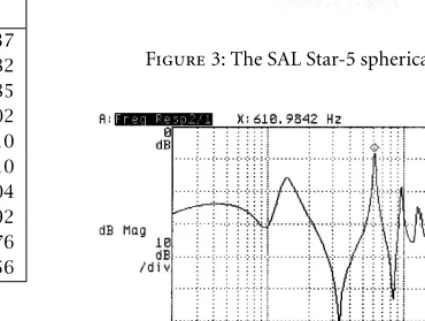
The resonant frequencies of the spherical loudspeaker depicted in Figure 3 were measured. In this loudspeaker 12 low-frequency as well as 20 high-frequency transducers are mounted on a spherical ABS plastic enclosure. (We thank Speaker Array Logic for providing the loudspeaker.) Several resonances could be identified with sufficient accuracy (see Figures 4, 5, and Table 4) [12]).
The resonances of an inflatable plastic ball having a di-ameter of 0.67m were also measured by posing the plastic ball onto a small loudspeaker. The loudspeaker was playing test signals through the ball and a microphone recorded the
Figure3: The SAL Star-5 spherical loudspeaker.
Figure4: Frequency response measured within the enclosure of the spherical loudspeaker.f11can clearly be identified at611Hz.
sound filtered by the ball (Figure 14) at the temperature of 23◦C degrees. The position of the microphone was chosen
in order to balance the amplitude of the various resonances. A spurious resonance showed up at200Hz, probably due to the imperfect coupling between the loudspeaker and the ball, so that it was necessary to prefilter the excitation signal with a parametric notch equalizer tuned at200Hz.
Figure5: Close up of Figure 4 between500Hz and2500Hz. Six resonances can be identified.
Table4: Resonances of the spherical loudspeaker Star-5. (fm)
mea-sured frequency, (fth) is the theoretical value, (up) is the sharpness.
The theoretical values are computed for a radius of0.188m and a temperature oft=25◦C.
fns fm(Hz) fth(Hz) up%
f02 1290 1319 −2
f11 615 611 1
f22 960 981 −2
f32 1350 1325 2
f42 1680 1657 1
f52 2000 1983 1
f62 2240 2304 −3
withf11,f22,f32,f42,f52,f62,f72, andf92.
5. SPHERICAL RESONATOR MODEL
The first attempt to imitate spherical resonators, as shown in Figure 2, has provided audible results that allow users to distinguish simulated spheres from other shapes such as cube, quader or tube just from their specific sound colour. This seems to confirm experiments on object recog-nition performed with blind subjects [13]. From the AML model, we have learnt that the fundamental frequencies (f11, f22, f32, . . . , fn2) should be modelled with a high accu-racy. The periodic spacing of resonances at higher frequencies is an effective parameter but it is difficult to tune. If all the resonances were spaced according to the asymptotic spacing
πof theznsroots, they would imitate a cylinder rather than a sphere. On the other hand, the spacing at low frequencies is much larger than the asymptotic spacing (Table 2), so the spacing was tuned empirically at an intermediate value. In the early experiment, theznswere grouped according to the numbersof the roots rather than to the ordernof the func-tion because we noticed that the spacing in theznsseries was more regular alongsthan alongn.
Building on the experience gathered with this first model,
Table5: Resonances of the0.67m plastic ball. (fm) is the measured
frequency, (fth) is the theoretical value, (up) is the sharpness. The
theoretical values are computed for a diameter of0.673m and a temperature oft=23◦C.
fns fm(Hz) fth(Hz) up%
f11 400 340 17.0
f22 588 546 7.7
f32 772 738 4.6
f42 944 923 2.3
f52 1120 1104 1.5
f62 1306 1283 1.8
f72 1470 1460 0.7
f92 1810 1810 0.0
Frequency
Phase
in
ra
dians
−10π −8π −6π −4π −2π 0
Allpass filter phase response
Pure delay phase response
Target phase response
Target resonance frequencies
Figure6: Simplified view of the phase response of the inharmonic comb filter loop associated with a Bessel function. It is shown how this phase response can be constructed as the sum of the contribu-tion of a pure delay with the phase response of an allpass filter.
we try here to design a more systematic one. Consider the perfectly-reflecting rectangular box and its representation in the BaBo model. Let us see how the model can be extended to spherical enclosures.
Indeed we would like to consider a perfectly reflecting sphere as a parallel connection of nonharmonic comb filters. The resonances of thenth comb filter correspond to the local extremal points of thenth order spherical Bessel function. A first trade-off of our design is the highest ordernof the Bessel functions that is considered.
contribu-+
Figure 7: Inharmonic comb filter reproducing the modal reso-nances associated with a Bessel function of a given order.
(a)
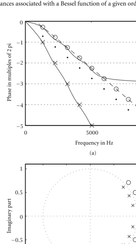
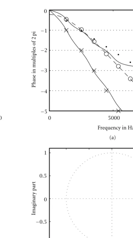
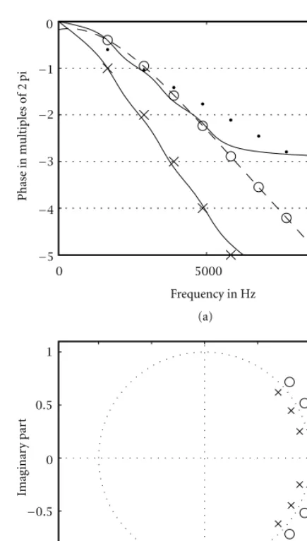
Figure8: (a) Phase response of the feedback loop of a inharmonic comb filter reproducing the resonances of a spherical resonator (r=
0.188m) associated with the Bessel function of order0:×: phase response at resonance points;•: phase provided by the delay (8 samples);◦: target phase residue to be approximated by the allpass filter; dashed line: polynomial curve approximating the target phase points; solid lines: designed allpass filter phase response and overall approximated phase response. (b) Pole-zero plot of the designed allpass filter.
tion (that can be approximated by a stable allpass filter). The scheme of one of the inharmonic comb filters is shown in
(a)
Figure9: Same parameters as Figure 8. Bessel function of order 1.
Figure 7, where the allpass filter and delay line are the main components of the feedback loop. In a practical implemen-tation, one should also include a lowpass filter that accounts for frequency-dependent losses in a modal series. Such a filter can be designed starting from measured modal decay times. Alternatively, its parameters can be left open to user adjust-ment. In any case, we are neglecting losses at this stage, as we are mainly interested in the frequency distribution of reso-nances rather than in their relative strength.
(a)
Figure 10: Same parameters as Figure 8. Bessel function of order 2.
given by a delay line whose length is equal to the slope of the linear ramp, and the nonlinear residual can be provided by an allpass filter.
A second design trade off appears here: up to which num-berSshould thefns,0≤s≤S, be approximated? Measure-ments and computations show that it is rather difficult to identifyfns,s >1resonances since slight inaccuracies suffice to change assignements. The experience gained in the first model (Figure 2) indicates thatS cannot be too small if the “sense of roundness” has to be maintained in the medium and high frequency range. The order chosen for the allpass filter will determine the numberSof resonances that will be accurately imitated.
The nonlinear phase curve can be roughly approximated by a couple of linear segments, a low-frequency slope and a high-frequency slope. With this observation, the allpass filter for the0order Bessel function can be designed by placing the poles on the unit circle according to these two slopes.
(a)
Figure11: Same parameters as Figure 8. Bessel function of order 3.
Figure 8(b) shows a zero-pole distribution that gives the two-slope phase response interpolating the small circles, which is depicted in solid line in Figure 8(a). Figures 9 to 12 show the phase responses and pole-zero plots for the same sphere as in Figure 8, but with a Bessel function order going from 1 to 4. Table 6 shows the designed parameters for radius equal to 0.188m and0.32m, and Bessel functions going from0to2. Reasonably shaped allpass phase responses can be obtained just by controlling two parameters, the argument of the first (low-frequency) pole, and the angular distance between any couple of contiguous poles.
6. DESIGN PROCEDURE AND EXAMPLES
low-(a)
Figure12: Same parameters as Figure 8. Bessel function of order 4.
frequency pole and the relative distance between all the other equidistant poles. The relative contribution of the delay line to the loop phase response is also subject to optimization. The distance of the poles from the centre is kept fixed as it is mainly responsible for the magnitude of the ripples in the phase response. This pole radius plays a minor role be-cause we are not interested in the phase values between the positions of resonance peaks and, therefore, we are not inter-ested in a particular value of the phase ripples. A criterion for choosing the initial inter-pole distance is that the asymptotic distance between the peaks associated with a Bessel func-tion is equal to a period of the ripple. The error that the iterative design procedure tries to minimize is the sum of the square phase differences at the target resonance points, weighted by some monotonically decreasing function that allows a more accurate positioning of resonances in low fre-quency.
If the goal is having a spherical resonator model that can be controlled in its radius, the design procedure should be
run several times, each for a selected value of radius. In this way, a table can be constructed with a complete set of param-eters for the resulting inharmonic comb filters. Notice that, even though a sixth-order allpass filter has six coefficients, the observation made in Section 5 allows us to implement it as three second-order sections that can be controlled by two pa-rameters: the angle of the first pole, and the angular distance of the following poles. The results of the design procedure for two distinct radii are reported in Table 6. Since the precise position of resonances is of some importance only in the first few thousands Hz (say,4kHz) [14], we see that a low order allpass filter is adequate for small spheres, e.g. order6or less for radii smaller than0.5m. However, for larger spheres, the filter order should be increased in order to provide a decent approximation at least under the first kHz.
Table6: Parameters for the inharmonic comb filter. Bessel functions of order 0 to 2.
radius knee slope angle separ. delay fund. freq. [m] [rad/s] (×10−16) 1st pole angle [kHz]
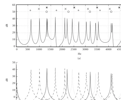
Figure 13(a) shows the frequency response of the par-allel connection of dispersive comb filters, here designed for radius0.188m. The marks represent the ideal modal positions for Bessel functions of order 0 to 3. In order to have a good match between the first resonance of each comb and its theoretical position, we properly shaped a weighting function to be used in the iterative optimization procedure. Maximum weight is used around the first res-onance, while the following resonances become gradually less important. Psychoacoustic investigations should be con-ducted in order to better understand if the approximations introduced can be perceived and if they affect the perceived object shape. However, informal listening seems to indicate that significant deviations from the theoretical partial posi-tions can be tolerated without loosing the “sense of round-ness.” For instance, the sharpness of resonances measured in the plastic ball, and reported in Table 5, does not seem to prevent the listener from identifying the enclosure as a sphere.
lo-(a) Hz
60
50
40
30
20
10
0
dB
0 500 1000 1500 2000 2500 3000 3500 4000 4500 5000
(b) Hz
50
40
30
20
10
0
−10
dB
0 500 1000 1500 2000 2500 3000 3500 4000 4500 5000
Figure13: (a) Frequency response of the parallel of dispersive comb filters designed for radius 0.188. Resonance positions of the ideal sphere are indicated for Bessel functions of order 0 (o), 1 (+), 2 (×), and 3 (*). (b) Superposition of the responses of dispersive comb filters for Bessel functions of order 0 (solid), 1 (dashed), 2 (dash-dotted), and 3 (dotted).
cal result is either a magnification or an attenuation of the peak. As well as with actual enclosures where the shape of the frequency response is dependent on the positions of exciter and pickup, with the FDN we can vary the shape of the re-sponse, without moving the resonances, just by changing the input and output coefficients [3], indicated asbi andci in Figure 1.
7. TRIALS, DISCUSSION, AND TUNING
The ability of a model to simulate actual objects can be checked by comparing sounds played through the real ob-jects with sounds processed by the model. Let us consider two different objects: a cylinder and a ball. Their shapes are far enough from each other to allow for a clear difference between processed sounds.
Figure 14 shows the setup used to record sounds pro-cessed by actual objects. The plastic ball is layed onto a small loudspeaker fed by a CD-player. Since the coupling be-tween loudspeaker and sphere provoques a strong resonance at200Hz, a notch filter is inserted between the sound source
and the loudspeaker. The microphone picks up the sound radiated in the recording room. In a similar fashion, sounds played in a tube closed at one end are recorded. Since the transducers and the room are not completely neutral, a third recording is made that serves as a reference: the sound played through the loudspeaker alone.
bright-CD
200Hz
DAT
CD
200Hz
DAT
CD
200Hz
DAT
1000
mm
1007
mm
E φ600/670mm
P
200 mm
(a) (b) (c)
Figure14: Measurement setup used for Figure 15. A sound is played from a CD-player through a loudspeaker. On top of the louspeaker, a sphere (b) or a tube (c) are posed. The sound modified by the shape, acting as a resonator, is recorded by a microphone. As a reference, the sound without any resonator is also recorded (a). A notch filter tuned at200Hz removes the disturbing resonance that appears when the sphere is coupled to the loudspeaker.
ness of the sounds played through the tube has been ad-justed by modifying the length of the tube until it empir-ically fits the brightness of the sounds played through the sphere.
Some listeners easily recognise the shape of the object just by listening to their sounds [9]. Most listeners agree that each object has a very peculiar sound colour but they fail at describing the differences and at telling one shape from the other. Many of them are capable of making a decision after a few learning trials, as if the knowledge had been available in their brain for a long time (perhaps since childhood) but that this knowledge had to be reacti-vated.
Similar tests were performed with sounds processed through the computer models. The FDN model of the sphere produces sounds with a refined reverberation, but the typical character of the sphere is less prominent. When comparing with FDN simulations of cubes, it is more difficult to tell the shape that is currently being simulated even though prior ex-posure still helps significantly. The fact that a sophisticated model performs worse than a simpler model for specific cases must be interpreted thinking that the initial model of the sphere (Figure 2) was constructed for a specific radius by fine tuning of a few prominent resonances. On the other hand, the FDN model aims at achieving generality and complex behaviour with a compact parametric structure. However, further research in sound perception has to be pursued in
order to understand which are the salient characteristics of a sound spectrum that bring us its shape signature. When such results become available, the design procedure of the FDN spherical model will be improved further.
7.1. Including deviations from the ideal, rigid sphere
The FDN has been optimized according to the theory of the sphere but, in order to compare it with the plastic ball, de-viations from the theoretical tuning had to be implemented. Such deviations (see Table 5) can be introduced in our model just by moving the theoretical resonance positions in the pro-cedure for designing the allpass filters. This can be done fairly easily if the deviations are small, otherwise it can be difficult to assign a certain resonance to an inharmonic comb series. Alternatively, one can start with the filters designed for the ideal sphere and adjust the position of the first pole, as we did to obtain the frequency response of Figure 16, which should be compared with Figure 15. In the feedback loop, we used second-order FIR filters (exhibiting a one-sample delay) to simulate the faster attenuation of higher modes. Moreover, a first-order lowpass filter has been cascaded with the whole structure in order to resemble the lowpass characteristic of Figure 15.
Figure15: Measured frequency response of the plastic ball.
Figure16: Frequency response of the FDN model of the plastic ball
+: resonance positions of the ideal sphere.×: measured resonance positions.
the physical theory of the sphere is not sufficient to drive the design stage, and perceptual issues should be considered. To this end, the issue of identifying a shape from its audible signature should be investigated more deeply in the future.
8. CONCLUSION AND FURTHER RESEARCH
We have shown that the basic structure of the BaBo model can also be used to simulate spherical geometries, just by using properly designed allpass filters within the filtering blocksHi
of Figure 1. The resulting model might be called “Ball within the Ball” (BaBa). We have shown that a simple design proce-dure and, possibly, some manual tweaking, allow an efficient structure to be realized that can be tuned either like an ideal sphere or like a real one. An open question is nevertheless how accurate this design has to be, since it is still unsettled which are the relevant parameters that affect the “perceived roundness” of the object.
An important aspect of the model is that very few param-eters are added to the BaBo model to control the allpass filters
of the spherical model. Even deviations from ideal boundary conditions are reasonably achieved by moving only the posi-tion of one pole per inharmonic series. So far, we have sim-ulated inharmonic series given by Bessel functions of order ranging from0to6. In many cases, higher order inharmonic series are needed to achieve realism, but the fundamental res-onance of those series seems to be most important while the higher resonances get drowned in the dense mixture of res-onances from other series and their position is out of the bandwidth of perceived inharmonicity. So, we suggest to im-plement higher-order series as harmonic comb filters tuned to the fundamental frequency of that series. Some form of delay interpolation [15] might be needed to position such fundamental frequencies with sufficient accuracy.
The same structure used for spherical resonators might be as well used for cylindrical resonators [10]. In this case there is a harmonic series given by longitudinal modes, superimposed with inharmonic series of resonances whose positions are de-termined by the extremal points of cylindrical Bessel func-tions. Therefore, the feedback delay network should have the first delay line accounting for the longitudinal modes, and the remaining lines, cascaded with properly-designed allpass fil-ters, accounting for the inharmonic, transversal modal series. If the inharmonic series, each corresponding to a Bessel function of a certain order, are recreated by comb filters hav-ing a delay line and an allpass filter in the feedback loop, it is conceivable to control the degree of “roundness” of the enclo-sure by changing the relative contribution to the overall phase response given by the delay and by the allpass filter. Namely, if all the delays are increased we gradually move from a sphere to a cube with rounded faces. This continuous shape con-trol, as well as the extension of the BaBo model to cylindrical shapes will be covered in future research.
REFERENCES
[1] J.-M. Jot, Etude et réalisation d’un spatialisateur de sons par modèles physiques et perceptifs, Ph.D. thesis, TELECOM, Paris 92 E 019, 1992.
[2] J.-M. Jot and A. Chaigne, “Digital delay networks for designing artificial reverberators,” inAudio Eng. Soc. Convention, Paris, France, AES, February 1991.
[3] D. Rocchesso, “The ball within the box: a sound-processing metaphor,”Computer Music J., vol. 19, no. 4, pp. 47–57, 1995. [4] D. Rocchesso and J. O. Smith, “Circulant and elliptic feedback delay networks for artificial reverberation,”IEEE Transactions on Speech and Audio Processing, vol. 5, no. 1, pp. 51–63, 1997. [5] H. Kuttruff,Room Acoustics, Elsevier Science, Essex, England,
3rd edition, 1991.
[6] J. A. Moorer, “About this reverberation business,” Computer Music J., vol. 3, no. 2, pp. 13–18, 1979.
[7] M. R. Schroeder and B. Logan, ““Colorless” artificial reverber-ation,”J. Audio Eng. Soc., vol. 9, pp. 192–197, 1961.
[8] P. M. Morse and K. U. Ingard,Theoretical Acoustics, McGraw-Hill, New York, 1968 reprinted in 1986, Princeton Univ. Press, Princeton, NJ.
[10] P. M. Morse, Vibration and Sound, American Institute of Physics for the Acoustical Society of America, New York, 1991. [11] M. R. Moldover, J. B. Mehl, and M. Greenspan, “Gas-filled spherical resonators: theory and experiment,”J. Acoustical Soc. of America, vol. 79, no. 2, pp. 253–272, 1986.
[12] J. Schwörer and P. Dutilleux, “Versuchsaufbau mit dem Kugel-lautsprecher SAL Star-5 in omnidirektionalem Betrieb,” Tech. Rep., ZKM: Zentrum für Kunst und Medientechnologie, Karl-sruhe, Germany, 1998.
[13] R. McGrath, T. Wildmann, and M. Fernström, “Listening to rooms and objects,” inConference on Spatial Sound Reproduc-tion, Rovaniemi, Finland, AES, 1999, pp. 512–522.
[14] D. Rocchesso and F. Scalcon, “Bandwidth of perceived inhar-monicity for physical modeling of dispersive strings,” IEEE Transactions on Speech and Audio Processing, vol. 7, no. 5, pp. 597–601, 1999.
[15] T. I. Laakso, V. Välimäki, M. Karjalainen, and U. K. Laine, “Splitting the unit delay—tools for fractional delay filter de-sign,”IEEE Signal Processing Magazine, vol. 13, no. 1, pp. 30–60, 1996.
Davide Rocchessoreceived the Laurea in In-gegneria Elettronica degree from the Univer-sity of Padova in 1992, and the Ph.D. de-gree from the same university in 1996. His Ph.D. research involved the design of struc-tures and algorithms based on feedback delay networks for sound processing applications. In 1994 and 1995 he was a visiting scholar at the Center for Computer Research in Mu-sic and Acoustics (CCRMA) at Stanford
Uni-versity. Since 1991 he has been collaborating with the Centro di Sonologia Computazionale (CSC) at the University of Padova as a researcher and a live-electronic designer. Since March 1998 he has been with the Dipartimento Scientifico e Tecnologico at the Uni-versity of Verona, as an Assistant Professor. His main interests are in sound processing, physical modeling, sound reverberation and spatialization, multimedia systems. His home page on the web is http://www.sci.univr.it/˜rocchess.
Pierre Dutilleuxgraduated in thermal
en-gineering from the ENSTIMD in Douai in 1983 and in information processing from the ENSERG in Grenoble in 1985. He developed audio and musical applications for the Syter real-time audio processing system designed at INA-GRM by J.-F. Allouis. After develop-ing a set of audio processdevelop-ing algorithms as well as implementing the first wavelet anal-yser on a signal processor, he got a Ph.D. in