A computing method for 3D magnetotelluric modelling directed by polynomials
Pierre-Andr´e Schnegg
Institute of Geology, CH-2007 Neuchˆatel, Switzerland
(Received November 2, 1998; Revised February 23, 1999; Accepted April 12, 1999)
A computational method for automatic 3D MT modelling is described. Making use of a recent publicly available forward algorithm, our method allows unattended search for a 3D conductivity model. The geometry of the conductivity features is described by a set of mathematical functions of the horizontal coordinatesxandyand of a fixed number of parameters. Starting from a presumed conductivity distribution, our scheme automatically varies the parameters in a steepest descent control loop, until the misfit between the model response and the measured data reaches an allowable value. To illustrate the method, we apply it to MT and induction data gathered in the Swiss Alps and determine the depth and lateral extension of a highly conductive, graphite-bearing layer.
1.
Introduction
When an efficient new numerical algorithm to compute two-dimensional (2D) magnetotelluric problems was pub-lished (Wannamakeret al., 1985), it was immediately used by many induction researchers to improve their modelling results. They suddenly had the opportunity to add a new dimension to earlier simplistic 1D models. However, with the then available computing power, 2D modelling was a very lengthy process. At each step of the modelling, after a small variation of the conductivity distribution had been introduced, it was necessary to carefully re-design the finite-element mesh. In the last ten years, however, a wealth of 2D automatic schemes has appeared, relieving the researchers of the most tedious part of their work (Jones, 1993).
Similar situation occurred with the advent of 3D schemes. So far researchers have carried out 3D modelling in very lengthy ways, manually changing the parameters of their conductivity models until they were finally satisfied with the results. To make the search for the best model a smoother, more unattended work, we had the idea of incorporating the code of a forward 3D MT field computation scheme into a main computer programme which would handle most of the repetitive task. Once a model topology has been cho-sen by the operator (number of layers and possibly, number of isolated conductive or resistive features), the programme automatically handles most of the tedious operations like mesh design, calculation of misfit between measured data and model response, and parameter fitting. At each itera-tion our programme calls the forward calculaitera-tion routine. Because all five EM field components can be computed in the forward code, it becomes possible to search conductivity models with any subset of MT parameters (one or two MT polarisations and/or vertical magnetic field) or with all of them in the calculation of the objective function.
Copy right cThe Society of Geomagnetism and Earth, Planetary and Space Sciences (SGEPSS); The Seismological Society of Japan; The Volcanological Society of Japan; The Geodetic Society of Japan; The Japanese Society for Planetary Sciences.
2.
Method Description
The forward calculation used in our 3D MT modelling scheme was developed and made available in the last few years (Mackieet al., 1993, 1994). This calculation is based on the integral form of Maxwell’s equations where acceler-ated conjugate gradient relaxation is used to solve for the magnetic field Hx,HyandHz. Mackie’s new forward tech-nique and the tremendous increase of available PC computing throughput have given rise to numerous studies addressing three-dimensional lithologies. Examples of such studies can be found in (Pous et al., 1995; Livelybrookset al., 1996; Maseroet al., 1997; Park and Mackie, 1997). However, it seems that none of these modelling attempts used fully auto-matic methods. Because they require much control from the operator, their result may be unconsciously biased toward more or less subjective final models. The scheme implied in our method is probably less subjective since it requires less intervention (initial parameterisation must still be done by the operator, however). It differs little from an approach used in a previous work on 2D MT modelling (Schnegg, 1993; Schnegg, 1996), where the shape and resistivity of a conducting structure is bounded by a set of simple polyno-mial functions of the profile distance.
There will be no further mention of the maths involved in the method of Mackieet al. (1993). The idea behind our tech-nique is the control of the construction of a 3D model with a finite set of smoothly varying functions of the space coordi-nates. Useless to say, construction must respect some design rules so that at the end, the model fits the format required by the forward modelling scheme used (Mackie and Madden, 1994). The resistivity of the elementary 3D blocks of the regularisation mesh is controlled by these smooth functions. In this paper, simple polynomial functions of the coordinates are chosen, but obviously other analytic, continuous func-tions could do as well. Our method has certain similarities to Occam’s 2D inversion (de Groot-Hedlin and Constable, 1990). Occam’s inversion seeks structures with minimum roughness in both horizontal and vertical directions. In our
method, the polynomials ensure smoothness within a given layer, but the whole design enforces vertical layering. Keep-ing the number of parameters close to the number of sites avoids overinterpretation of the data, suggesting the real resolving power of the magnetotelluric soundings. In the present scheme, a conductivity distribution will be described by a stack ofNlayers. Although we can easily imagine thick lithologies without any stratification, most of the time the ge-ology of a given area assumes strong layering. Such prior geological knowledge, if it exists, can be used to constrain the minimisation of an objective function based on data-misfit (Ellis and Oldenburg, 1994). The logarithms of the layer thicknesses assume a polynomial form described by a set of
Ngiven functions of the horizontal coordinatesξ andψ.
Fj(ξ, ψ,pi), i=1, nj, j=1, N−1. (1)
Within each layer in turn, the logarithm of the resistivity can be set to afixed value but more generally, will also be varying as a polynomial function of the coordinates
Fj(ξ, ψ,pi), i =1, nj, j =N, 2N−1. (2)
Note that the description of both thickness and resistivity occurs in logarithmic space. The reason for this apparently useless complexity is to avoid zero crossing of the parameters during their variation by the minimising routine, which can only progress stepwise. Working with logarithms has the additional advantage of enabling more rapid (exponential) variations of the parameters than direct values would do.
In the general case, variablesξ andψare curvilinear co-ordinates, but they could also be chosen as simple Cartesian coordinatesxandyon the horizontal surface of the Earth (x
toward theN,ytoward theE). Each functionFjdepends on
nj parameters pi. In the simple case of polynomials, these parameters are the multiplying coefficients of the termsx,y,
x2,x y,. . .. For instance, in the case of a representation with
3rd-degree polynomials the thickness of thefirst layer would be written as
h1 =10p1+p2x+p3y+p4x
2+p
5x y+p6y2+p7x3+p8x2y+p9x y2+p10y3. (3) Let us now consider Mackie’s regularisation mesh. Its central part contains a stack of small 3D blocks of dimensions
x,y,z. There is provision for horizontal variation of the cell dimensions. A given horizontal slice has afixed vertical thickness, but this parameter is allowed to vary vertically from one slice to the next. Three-dimensionality is restricted to the model core. The outer parts are 2D and 1D structures extending the regional features.
Our conductivity model is discretized in the same way, keeping this timexandyconstant within a given slice. The vertical cell dimensionzmay be kept constant or al-lowed to increase exponentially with depth. Two-D and 1D edges are also included in the model. They insure correct boundary conditions both laterally and vertically. Conse-quently, the range of influence of the polynomials is restricted to the inner 3D part of the model. During the successive steps of our directed forward modelling, the shape and dimensions of the 3D regularisation mesh stays unchanged. The model variation is entirely controlled by the resistivity variations of
the building blocks. Each elementary block belongs to one of the N layers and thus can be given the resistivity of that layer, which depends on the polynomialsFj.
Our scheme automatically varies the parameters pi and checks the result improvement in terms of least squares misfit between model response and measured data. Both phaseφ and logarithm of the apparent resistivityρa are used in this computation according to Eq. (4) (Fischer and Le Quang, 1981): where the indicesmandcrefer to measured and calculated data,wρi andwφi represent the data weights andTi are the
N periods for which measured data are available. Misfit
decreases because the search progresses in the direction of steepest descent in the parameter space. After a certain number of iterations we end up with the best model (in terms of data fit) that can be represented with the selected set of functionsFj. In fact, the calculation is stopped once afixed maximum allowable misfit threshold is reached. Unfortu-nately there is no guarantee that the absolute minimum misfit has been obtained. Sometimes it is more convenient tofix a time limit to the modelling. Depending on the assumed topology of the target geology, it is up to the modeller to select the set of functions which he believes will bestfit the problem. These functions can extend from simple polyno-mials of x and y(in the case of distorted dipping layered structure), to any combination of orthogonal polynomials, like spherical harmonics and Legendre polynomials (which would be required for axi-symmetric geometries found in geological features like salt domes, volcanoes with magma chambers, astroblems, etc.). Obviously, once a set of func-tions has been selected, the model will only assume limited freedom of topological variation, since the search is done on the parameterspionly, and not on the kind of function itself. There is an important trade-off in the search for the best model: On one hand, the conductivity distribution must be described by as many parameters as required tofit the data. On the other hand, this number must be kept within rea-sonably small values (practically smaller than 20) to avoid convergence problems caused by computing time limitations. Moreover, too many parameters would smooth out the param-eter space and turn a deep absolute minimum into numerous shallower valleys.
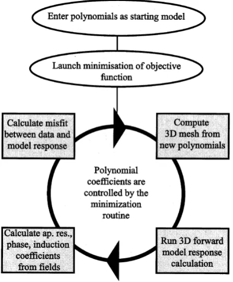
The programmeflowchart is shown in Fig. 1. First thefield data and initial values of the model parameters are read in. At this stage preliminary information delivered by other meth-ods (1D and 2D magnetotellurics, seismic lines, gravimetry) can be advantageously introduced to help design the starting model. Using weights will allow individual adjustment of parameter sensitivities. They can be set to zero to freeze the variation of a given parameter, permitting the application of deliberate constraints on the modelling process.
Fig. 1. Programmeflowchart.
criterion is not met. As usual, the misfit is the error between the measured data and the model response, summed over all measuring sites, periods, and MT parameters (2 MT polari-sations and/or vertical magneticfield), including apparent re-sistivities, induction coefficients and their respective phases. Weights computed from the error bars can be attributed to individualfield data to take their quality into account.
At the end of each cycle, a new conductivity model is de-signed by the programme. This step is carried out according to Mackie’s recommendations for mesh design. Mackie’s method divides space into cells of parallelepiped shape. To design the new model, the value of the resistivity of the cells at coordinatesxandyare computed by the proper selected set of functions Fj. These functions, in turn, can be com-puted with the parameters proposed by the minimising rou-tine. Then a forward calculation of the model response can be performed. In terms of computing time, this last step is effectively the most demanding part of the code. Once avail-able, model responses are compared to measured data and a misfit value is derived. Finally the minimising routine can use the information on the misfit variation to modify the pa-rameter set and determine the direction of steepest descent toward convergence in parameter space. Since there is no need for human control during the process, the computation can run unattended for several hours or days.
3.
Minimisation Routine
Our minimisation procedure MINDEF (Beiner, 1970) al-lows tofind a relative minimum of any real functionFof as many as 30 variables. The procedure is optimised in such a way that the number of calls of the function F is kept to
a minimum. Moreover, the derivative of F is not required. The search for a minimum is carried out in three steps: 1) varying the parameters around the starting point until a di-rection of descent is found. 2) progression in the descent direction. 3) as soon as the progression fails, parameters are varied into the space perpendicular to the progression, try-ing thus tofind a breakthrough. The same ternary strategy is repeated automatically from the last point as long as an acceptable minimum is not found. In our application we use the RMS value computed between the measured data and the model function as the objective functionFto minimise.
4.
Field Example
To illustrate the method on real MT and GDSfield data, we use the results of a recent survey carried out in the Penninic Alps of Valais, Switzerland (Schnegg, 1998). MT and ver-tical magneticfield data were recorded at 24 sites scattered over an area of 60×40 km. The Rhone valley represents a natural separation between the external,“helvetic”and in-ternal “penninic” zone of the Central Alps. The helvetic domain corresponds to the South-eastern edge of the former European continent. The penninic zone, on the other hand, consists of a complex stack of basement scales and cover nappes. Of particular interest to our study is the deepest, northernmost nappe called“Zone Houill`ere”. The high car-bon content of this nappe makes it a good candidate for a conductivity anomaly. Moreover, this lithology crops out at the surface along the Rhone river. Laboratory study of drill cores from a nearby borehole confirmed the presence of low-grade carbonated material. Sample measurements revealed resistivities of as low as 0.6m. Conductivity increase with hydrostatic pressure is likely to indicate reconnection of car-bonfilms at the grain boundaries (Glover and Vine, 1992).
Using our 2D modelling method (Schnegg, 1993), a pre-liminary search for a 2D model was carried out with a sub-set of sites selected in the neighbourhood of a well-centred profile line. This revealed the shape and extension of a
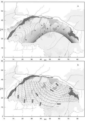
Fig. 3. 3D MT/GDSfinal model after 400 iterations. (a) Isolines of the depth to the 0.2m body (km). (b) Isolines of the lateral resistivity distribution in the top layer (solid line) and third layer (broken line) inm. Graphite-bearing Zone Houill`ere outcrop is represented in dark.
ducting dipping slab, embedded in a resistive rock matrix. We used this 2D model to built the starting model of a 3D modelling. Figure 2 represents the polynomial envelope of the conductive slab. The region of study was subdivided into 24×14×20 parallelepipedic cells of size 3×3×0.5 km. Three columns and three rows were appended on each external face of the model, with increasing width of 6, 12 and 24 km, thus dividing the space into 30×20×20 blocks. Each vertical slice of this model was embedded in a larger 2D model which extended the regional features. A 1D structure (a half-space in this case) was added at the bottom. This mesh geometry did not vary during the entire modelling process. Only the cell resistivities were allowed to change.
According to the results of the 2D modelling, we restricted
would have been very difficult to resolve simultaneously the thickness and the resistivity of such a high conducting layer. This difficulty already appeared while carrying out the 2D modelling. Hence, the parameters which were automatically
fitted by our programme are the pi,qi andri which appear in the decimal logarithms of
1) the slab depth (or the thickness of first layer),
f1(x,y,pi,i =1,n1),
2) the resistivity of the rock matrix above the slab,
f2(x,y,qi,i =1,n2),
3) the resistivity of the rock matrix beneath the slab,
f3(x,y,ri,i =1,n3).
We used logarithmic values instead of the values themselves to prevent the resistivity and the thickness from becoming negative during the parameter control by the minimising rou-tine. These model parameters have been chosen to be simple polynomials of the coordinatesxandywith degrees set as high as possible with regard to the available computing re-sources, to 3, 2 and 2 respectively. If computing time would not be an issue, the upper limit of the polynomial order should have beenfitted to the measuring site density. No vertical resistivity variation was allowed within a given layer. As ini-tial values, f1was set to the logarithm of the 2D slab depth,
whereas constant polynomials were chosen for f2 and f3.
Thus, the three polynomials
have been selected to describe the conductivity distribution of the 3D part of our model.
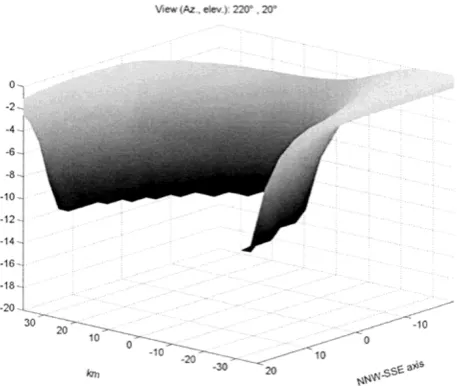
We carried out a joint modelling of the induction coeffi -cients of the measured vertical magneticfield, and the appar-ent resistivities and phases computed from the MT matrix rotated into the directions of the axes of Fig. 2. Because computing time is proportional to the number of periods at which the misfit is computed, we had to restrict the dataset to periods of 1 and 100 seconds. However, these periods could be shown in the 2D modelling to be well suited and representative of the studied conductivity environment. Iso-lines of the depth of the conducting slab after 400 iterations are shown in Fig. 3 and a 3D view in Fig. 4. Note that the smooth surface displayed in Fig. 4 is not an image of the true conductivity distribution of the model, but rather its poly-nomial envelope. It should be reminded that the model is a juxtaposition of small blocks. However, we have some reason to believe that the real shape of the conductive slab resembles more a smooth structure than a blocky one. The
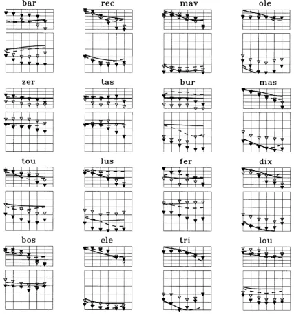
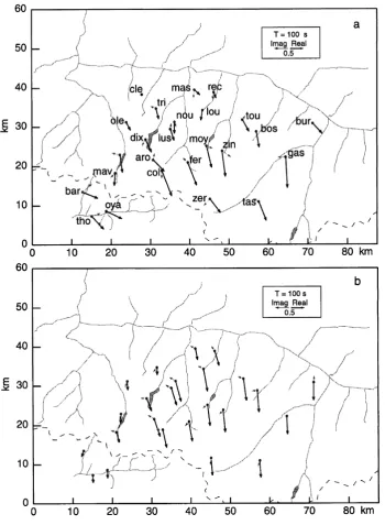
final model response is compared with thefield data in Fig. 5 (MT apparent resistivities and phases) and Fig. 6 (induction arrows). Note that Fig. 5 displays data points at all mea-sured periods, in spite of the limitation to only two of them which were effectively used in the modelling. The full lines denote the model response calculated at periods of 1, 3, 10, 30, 100 and 300 seconds and interpolated. On the contrary,
Fig. 4. Polynomial envelope of the high-conducting (0.2m) slab of
final model after 400 iterations. Logarithm of thickness offirst layer is described by a 3rd-degree polynomial ofxandy:
p1+p2x+p3y+p4x2+p5x y+p6y2+p7x3+p8x2y+p9x y2+p10y3. Logarithmic scale is used to prevent the thickness from being negative. Slab thickness was keptfixed at 1 km, according to the results of an existing seismic line.
Fig. 6 shows only the results at one period (100 s), although a second period (1 s) was also used in the search.
Obviously, the result of our 3D modelling must be re-garded as semi-quantitative only, since many simplifications were required to lighten the computing task (constant thick-ness and constant resistivity of the slab). However thefinal model clearly indicates that the shape of the conducting slab strongly departs from the cylindrical geometry suggested by the 2D model, closely matching the uppermost crustal boundary as determined by seismic profiles (Valasek, 1997). Moreover, a recent airborne gravimetric survey of the area (Klingel`e et al., 1996) shows a deep (30 mgal) local max-imum with a lateral extension exactly matching the bowl-shaped depression of our model. There is no doubt that the real shape of the conducting body is more complicated than can be described by our 3D model. In particular, a higher polynomial degree would be required tofit data from the SW edge. However, the general trend should not differ signif-icantly from reality, since it displays the same curvature as the Alpine arc, showing a marked depression. These match the large scale geometry of tectonic units bordered by fea-tures such as the external crystalline massif domes, the Rawil saddle to the NW, and the Insubric backfold to the SE.
Fig. 5. Measured apparent resistivity and phase (triangles) compared tofinal model response (lines) for two polarisations. Logarithm of period ranges from 0 to 3 (abscissa). Logarithm of apparent resistivity varies between 0 and 5. Phase axis varies between 0 and 90. Filled symbols and dashed lines denote the mode in which electric currentsflow parallel to the Rhone valley. Site locations are shown on the map of Fig. 6a.
5.
Programming Considerations
As was discussed already, continuous geological features can be described by simple polynomials, which are smoothly varying functions. Horizontal boundaries are easily repre-sented by such functions. Lateral variations of the resistivity can also be approximated by polynomials, provided there are no sharp resistivity variations as would result from the occur-rence of dikes, faults and similar tectonic features. Known lithologies with such high resistivity gradients can neverthe-less be modelled, at the expense of additional parameters. However, the number of freely varying parameters must be kept within reasonable limits for computing time considera-tions. Geological features with a vertical axis of symmetry (salt domes, volcanoes, astroblems, etc.) should be manage-able targets in an approach based on the use of Legendre
polynomials. Thefinal result of the present method is a set of parameters which control continuous functions of the co-ordinates, such as polynomials. The 3D forward modelling scheme does not compute the response of the continuous conductivity distribution specified by the polynomials, but the response of the blocky model inscribed in them.
6.
Conclusion
Fig. 6. Real and imaginary induction arrows at 100 s for (a) measured data and (b) response of model shown in Figs. 3 and 4.
Every smooth geological situation without lateral discon-tinuities of the resistivity can be approximated by simple polynomial expressions. This is particularly the case for structures produced in collisions (or extensions; suture zones, crustal d`ecollements and shear zones). Discontinuities can be dealt with by combining several polynomials, or by adding appropriate boundary conditions, at the expense of an en-hanced computing task, however. Finally, problems with axes of symmetry can also be treated. In each case, a proper choice of primitive functions is mandatory to obtain success-ful modelling results.
References
Beiner, J.,FORTRAN Routine MINDEF for Function Minimization, 5 pp., Institut de Physique, Univ. of Neuchatel, Switzerland, 1970.
de Groot-Hedlin, C. D. and S. C. Constable, Occam’s inversion to generate smooth, two-dimensional models from magnetotelluric data,Geophysics,
55(12), 1613–1624, 1990.
Ellis, R. G. and D. W. Oldenburg, Applied geophysical inversion,Geophys. J. Int.,116, 5–11, 1994.
Fischer, G. and B. V. Le Quang, Topography and minimization of the stan-dard deviation in one-dimensional magnetotelluric modelling,Geophys. J. R. astr. Soc.,67, 279–292, 1981.
Glover, P. W. J. and F. J. Vine, Electrical conductivity of carbon-bearing granulite at raised temperatures and pressures,Nature,360, 723–726, 1992.
Jones, A. G., The Coprod2 Dataset: Tectonic Setting, Recorded MT Data, and Comparison of Models,J. Geomag. Geoelectr.,45, 933–955, 1993. Klingele, E., M. Cocard, M. Halliday, and H.-G. Kahle,´ The Airborne
Gravi-metric Survey of Switzerland, Mat´eriaux pour la G´eologie de la Suisse, 31, 104 pp., Swiss Geophysical Commission, 1996.
Livelybrooks, D., M. Mareschal, E. Blais, and J. T. Smith, Magnetotelluric delineation of the Trillabelle massive sulfide body in Sudbury, Ontario, Geophysics,61(4), 971–986, 1996.
Mackie, R. L., T. R. Madden, and P. E. Wannamaker, Three-dimensional magnetotelluric modeling using difference equations—theory and com-parison to integral equation solutions,Geophysics,58, 215–226, 1993. Mackie, R. L., J. T. Smith, and T. R. Madden, Three-dimensional
electro-magnetic modeling usingfinite difference equations: the magnetotelluric example,Radio Sci., 923–935, 1994.
Masero, W., G. Fischer, and P.-A. Schnegg, Crustal deformation in the region of the Araguainha impact, Brazil,Phys. Earth Planet. Inter.,101, 271–289, 1997.
Park, S. K. and R. J. Mackie, Crustal structure at Nanga Parbat, northern Pakistan, from magnetotelluric soundings,Geophys. Res. Lett. (USA), 24(19), 2415–2418, 1997.
Pous, J., C. Ayala, J. Ledo, A. Marcuello, and F. Sabat, 3D modelling of magnetotelluric and gravity data of Mallorca island (Western Mediter-ranean),Geophys. Res. Lett. (USA),22(6), 735–738, 1995.
Schnegg, P.-A., An Automatic Scheme for 2-D Magnetotelluric Modelling, Based on Low-Order Polynomial Fitting,J. Geomag. Geoelectr.,45(9), 1039–1043, 1993.
Schnegg, P.-A., Comparison of 2D modelling methods: rapid inversion vs polynomialfitting, inElektromagnetische Tiefenforschung, edited by K. Bahr and A. Junge, pp. 74–79, Deutsche Geophysikalische Gesellschaft, Burg Ludwigstein, 1996.
Schnegg, P.-A.,The Magnetotelluric Survey of the Penninic Alps of Valais, Materiaux pour la G´ ´eologie de la Suisse,32, 76 pp., Swiss Geophysical Commission, 1998.
Valasek, P. and St. Mueller,A 3D Crustal Model of the Swiss Alps Based on an Integrated Interpretation of Seismic Refraction and NRP 20 Seis-mic Reflection Data, Deep structure of the Swiss Alps, pp. 305–326, Birkhauser Verlag, 1997.¨
Wannamaker, P. E., J. A. Stodt, and L. Rijo, PW2D-finite element program for solution of magnetotelluric responses of two-dimensional earth resis-tivity structure,Earth Science Laboratory, University of Utah, Salt Lake City, 1985.