R E S E A R C H
Open Access
On muting mobile terminals for uplink
interference mitigation in
HetNets—system-level analysis via
stochastic geometry
Francisco Javier Martín
3, Xiaojun Xi
2, Marco Di Renzo
2*, Mari Carmen Aguayo-Torres
1and Gerardo Gomez
1Abstract
We investigate the performance of a scheduling algorithm where the mobile terminals (MTs) may be turned off if they cause a level of interference greater than a given threshold. This approach, which is referred to as interference aware muting (IAM), may be regarded as an interference-aware scheme that is aimed to reduce the level of interference. We analyze its performance with the aid of stochastic geometry and compare it against other interference-unaware and interference-aware schemes, where the level of interference is kept under control in the power control scheme itself rather than in the scheduling process. IAM is studied in terms of average transmit power, mean and variance of the interference, coverage probability, spectral efficiency (SE), and binary rate (BR), which accounts for the amount of resources allocated to the typical MT. Simplified expressions of SE and BR for adaptive modulation and coding schemes are proposed, which better characterize practical communication systems. Our system-level analysis unveils that IAM increases the BR and reduces the mean and variance of the interference. It is proved that an operating regime exists, where the performance of IAM is independent of the cell association criterion, which simplifies the joint design of uplink and downlink transmissions.
Keywords: Cellular networks, Scheduling, Stochastic geometry
1 Methods/experimental
The methods used in the paper are based on the mathe-matical tools of point processes and stochastic geometry. A new analytical framework for performance analysis is introduced. The theoretical frameworks are validated against Monte Carlo simulations.
2 Introduction
Interference awareness can be exploited at both the physical and medium access control (MAC) layers to boost the performance of mobile networks. It is espe-cially useful in the uplink (UL) of heterogeneous cellular networks (HCNs) for interference mitigation and perfor-mance enhancement.
*Correspondence:[email protected]
2Laboratoire des Signaux et Systèmes, CNRS, CentraleSupelec, Univ Paris-Sud, Université Paris-Saclay, Paris, Gif-sur-Yvette, 91192 Paris, France
Full list of author information is available at the end of the article
In current HCNs, the mobile terminals (MTs) are asso-ciated with the same base station (BS) in the UL and downlink (DL) [1]. The cell association is performed based on DL pilot signals and the serving BS is chosen based on a given criterion, e.g., the highest average received power in the DL. In the UL, the same BS is used [1] which leads to a situation where MTs are associated with distant BSs. In this context, the use of fractional power control (FPC) accentuates the detrimental effect of the MTs that cause strong interference to neighboring BSs.
2.1 UL analysis: state-of-the-art
The aforementioned complex interactions between power control and association in the UL require accurate math-ematical frameworks to gain insights about the perfor-mance trends and limitations of existing and future net-works. Unfortunately, the mathematical analysis of the UL of HCNs is more involved than the analysis of the DL for
two main reasons: (i) due to the use of power control, the transmit power of the MTs depends on the distance to their serving BSs and (ii) even though the locations of BSs and MTs are drawn from two independent Pois-son point processes (PPPs), the locations of the interfering MTs scheduled in a given orthogonal resource block (RB) do not follow a PPP. These two peculiarities, as com-pared to the DL, make the mathematical analysis of the UL intractable without resorting to approximations [2]. In [3], the case of homogeneous cellular networks with FPC is studied. To avoid such a mathematical intractability, it is assumed that the MTs that are scheduled on a given RB form a Voronoi tessellation, and a single BS is available in each Voronoi cell. However, such an approach does not consider HCNs.
The case of the UL of HCNs is accurately modeled in recent works like [2,4–6], where the spatial correlation between the location of the probe BS and those of the interfering MTs is considered.
In [4], a framework to model HCNs with a truncated channel inversion power control under the smallest path loss association is introduced. In this work, a homoge-neous PPP is used as a generative process for the loca-tions of the interfering MTs, but the spatial correlation is accounted for by means of an indicator function that dis-cards interfering MTs’ locations based on their received powers.
The case of UL and DL with decoupled access is considered in [2]. The association is based on maxi-mum weighted received powers and FPC is considered in the UL. To account for the spatial correlations, a non-homogeneous PPP is considered to model the locations of the interfering MTs.
A framework for the UL of HCNs with multi-antenna BSs is studied in [5]. In this work, FPC is considered under a generalized association criteria and two extreme detection techniques in terms of complexity and per-formance: maximum-ratio combining (MRC) and opti-mum combining (OC). It is demonstrated that OC, which can be regarded as an interference-aware detec-tion technique for multi-antenna receivers, greatly out-performs MRC when MTs use aggressive power control, i.e., when the interference is high. The spatial corre-lation is imposed by means of a conditional thinning that takes into account the generalized cell association procedure.
Interference-awareness is also studied in [6], which considers HCNs with single-antenna BSs. In this work, a power control mechanism [7] is studied, which is referred to as interference aware fractional power con-trol (IAFPC). This approach consists of introducing a maximum interference level, i0, that the
transmis-sion of each MT is allowed to cause to its most interfered BS.
In simple terms, the MTs adjust their transmit power in order to cause a maximum interference level ofi0to their
most interfered BS.
In the present paper, we investigate another option for interference mitigation in the UL and compare it with previously reported schemes. The approach consists of exploiting interference-awareness when scheduling the transmission of the MTs, rather than in the power con-trol scheme itself (IAFPC) or in the detection process of the receiver (OC). As a result, interference management is conducted at the MAC layer rather than at the physical layer. The considered approach is referred to as interfer-ence aware muting (IAM) and consists of turning off, i.e., muting, the MTs whose interference towards the most interfered BS is above a given threshold.
The main difference between IAFPC and IAM can be summarized as follows. In IAFPC, all the MTs are active and adjust their transmit power for interference mitiga-tion. In IAM, on the other hand, the transmit power of the MTs does not account for any interference constraints but some MTs may not be allowed to transmit if they produce too much interference. As a result, IAM has the potential of reducing the aggregate interference in the UL and of enabling the active MTs to better use the available resources, i.e., the transmission bandwidth.
On the other hand, it reduces the fairness of allocat-ing the resources among the MTs, since some of them may be turned off. Nevertheless, thanks to mobility and shadowing, the muted MTs are only inactive for a given period of time. Hence, from the perspective of MTs, the question to answer is whether this muting increases its achievable binary rate (BR), taking into account both the active and inactive periods. In the present paper, this issue is analyzed as well, and some conclusions are drawn.
2.2 Technical contribution
The main objective of the present paper is to quantify the advantages and the limitations of IAM and compare it against the IAFPC scheme. This issue is, however, math-ematically challenging. In this paper, we overcome this mathematical intractability by using an approach similar to [5] and [6], which is referred to as conditional thin-ning. In simple terms, the locations of the active MTs are assumed to be drawn from a PPP but spatial con-straints (correlations) are introduced, which account for the location of the serving BS, for the location of the most interfered BS, and for the maximum level of interference allowed. Based on these modeling assumptions, which are validated against extensive Monte Carlo simulations, we provide the following contributions.
that IAM is capable of reducing the three latter performance metrics compared with IAFPC, which results in several advantages for practical
implementations.
Reducing the variance of the interference, e.g., is beneficial for better estimating the SINR and, thus, for reducing the error probability of practical decoding schemes, e.g., turbo decoding, [8], and for making easier the selection of the most appropriate modulation and coding scheme (MCS) to use in LTE systems [7].
• To make our study and conclusions directly applicable to current communication systems that are based on adaptive modulation and coding (AMC) transmission, we provide tractable expressions of SE and BR based on practical MCSs that are compliant with the LTE standard and whose parameters are obtained from a link-level simulator [9,10].
• With the aid of the proposed mathematical frameworks, we compare IAFPC and IAM schemes in terms of SE and BR, which provide information on their strengths and weaknesses. The SE provides information on how well the MTs exploit the available resources (e.g., bandwidth) that are shared among the MTs served by the same BS, whereas the BR accounts for the specific fraction of resources that is allocated to each MT served by a given BS. While the IAFPC scheme is superior in terms of SE, the IAM scheme is superior in terms of RB. This implies that IAM provides service to fewer users, which get better performance compared with IAFPC. To characterize this trade-off, we investigate the fairness of both schemes, which is defined as the probability that a randomly chosen MT gets access to the resources, and provide a tractable frameworks for its analysis.
• In light of the emerging UL-DL decoupling principle, we develop the mathematical frameworks for a general cell association (GCA) criterion, whose association weights may be appropriately optimized for performance enhancement. By direct inspection of the mathematical frameworks, we prove that three operating regimes can be identified as a function of the interference thresholdi0: (i) the first, where the
performance is independent ofi0, (ii) the second,
where the performance depends oni0but it does not
depend on the cell association, and iii) the third, where the performance depends oni0and the cell
association. Of particular interest in this paper is the second regime, which highlights that UL-DL decoupling may not be an issue for some system setups, which in turn simplifies the design of HCNs.
• As for the relevant case study for the UL where the serving BS of the typical MT is identified based on the smallest path loss association (SPLA) criterion
with channel inversion power control [1], we provide simple and closed-form frameworks for relevant performance indicators and prove that two operating regimes exist: (i) the first, where the performance depends oni0(interference-aware) and (ii) the
second, where the performance is independent ofi0
(interference-unaware). We prove, in addition, that (i) the scaling law of the average transmit power of the MTs, the mean interference, and the probability that a MT gets access to the resources is a polynomial function ofi0whose exponent depends on the path
loss exponent, (ii) the distance towards the serving BS gets smaller asi0increases, and (iii) the CCDF of the
SINR is independent of the density of BSs.
To the best of authors’ knowledge, all these contri-butions are new in the literature and are not included in previous works. For instance, the muting mechanism introduces further correlations that do not exist in [6] and need to be taken into account. This muting makes the whole analysis different. New metrics like the BR, which accounts for the amount of resources allocated by the scheduler, are obtained and a new framework to compute the SE and BR with AMC, which is closer to real sys-tems than Shannon formula, is introduced as well. Finally, closed-form expressions and remarks are obtained which provide important insights about system performance, fairness, and cell association.
The remainder of this paper is organized as fol-lows. Section 3 introduces the system model and the approach for system-level analysis. In Sections 4 and5, the analysis of IAM is presented for GCA and SPLA criteria, respectively. The BR of AMC schemes is ana-lyzed and discussed in Section 6. In Section 7, we introduce and study a hybrid scheme that allows us to overcome some fairness issues introduced by the IAM scheme. In Section 8, IAM and IAFPC schemes are compared against each other via numerical simu-lations and the main findings and performance trends derived in the paper are substantiated with the aid of Monte Carlo simulations. Finally, Section 9 concludes this paper.
Notation: A summary of the main symbols and
func-tions used throughout the present paper is provided in Table1for the convenience of the readers.
3 System model
We consider the UL of a HCN composed of two tiers,j∈
Table 1Summary of main symbols and functions used throughout the paper
Symbol/function Definition
2F1(·,·,·,·) Gauss hypergeometric function
K= {1, 2} Tier set: tier 1 is related to macro BSs, and tier 2 is related to small cell BSs
˜j= {k∈K:k=j} Complementary tier, i.e.,1˜ = 2 and2˜ = 1
(j),λ(j) PPP and its density related to the locations of
macro (j = 1) and small cell BSs (j = 2)
λMT Density of the PPP of MTs’ positions
,λ PPP and its density related to the locations of all BSs
t(j) Association weight for tierj
i0,p0,,pmax Interference threshold, target receive power, partial
compensation factor, and maximum transmit power
τ,α Path loss slope and path loss exponent
MT0, MTi Position of the probe MT and position of a generic
MT, e.g., an interfering MT
(k) PPP of interfering MTs’s locations R(xj,)(q) Distance (including shadowing) between
locationxand theqth nearest BS from tierj RMTi,UMTi,DMTi Distances (including shadowing) between MTi and
its serving BS, its most interfered BS and the probe BS
HMTi Power gain of the multi-path fading which is
exponentially distributed
pMT(r)=p0(τr)α Transmit power for a given distance towards the
serving BS for active MTs. Muted MTs has 0 transmit power
σ2
n,I Noise power and aggregate interference
according toAssumption1
X(j)
MTi Event defined as MTiis associated with tierj Q(m)
MTi Event defined as the most interfered BS of MTi belongs to tierm
X(j,m)
MTi Event defined as MTiis associated with tierj and the most interfered BS of MTibelongs to tierm
AMTi Event defined as MTiis active, i.e., non-muted AMTi Event defined as MTiis muted
O(j,k)
MTi Event defined as the interfering MTiof tier kreceives higher weighted average power from its serving BS than from the probe BS that belong to tierj
ZMTi Event defined as the interfering MTicauses a level of interference less thani0to the probe BS fX(·) PDF (Probability Density Function) of random
variableX
¯
FX(·) CCDF (Complementary Cumulative Distribution
Function) of random variableX LX(·) Laplace transform of random variableX
f(x0),f(x0) First and second derivatives of functionf(x)
evaluated atx=x0
E[·] , Pr(·),1(·) Expectation operator, probability measure and indicator function
(z), (a,z) Euler gamma function and incomplete gamma function
α >21. The cell association among MTs and BSs is based
on the weighted average received power criterion, similar to [2], where the association weights are denoted byt(j)for tierj∈K. Hence, theith MT is associated with thenth BS of tierjif the MT is in the weighted Voronoi cell of BS(nj)
with respect to = j∈K(j). With these assumptions, shadowing can be modeled as a random displacement [11] of(j)[6,12].
For ease of writing, we introduce the event XMT(j) i as follows:
Definition 1The eventXMT(j)
iis defined as “MTiis
asso-ciated with tier j.”
In mathematical terms, therefore, the association crite-rion can be formulated as follows:
X(j)
MTi=
t(j)
τR(MTj)
i,(1)
−α
>t(˜j)
τR(MT˜j)
i,(1)
−α
(1)
where(τRMT)−αis the path loss at a distance2RMTfrom
the transmitter,˜j=k∈K:k=jis the complementary tier ofj, i.e.,1˜ = 2, and2˜ = 1,R(x˜j,)(q)is the distance from
xto theqth nearest BS of tier˜j, i.e.,Rx(˜j,)(1)is the distance to the nearest BS. The association weightst(1)andt(2)allow us to model the GCA criterion, which encompasses the SPLA criterion fort(1)=t(2).
Throughout this paper, the analysis is performed for the probe or typical MT, i.e., for a randomly chosen MT, which is denoted by MT0. Its serving BS is referred to as the
probe BS.
3.1 Scheduling
We consider full-frequency reuse, where all the BSs share the same bandwidth. Each BS has available a bandwidth ofbwHertz that is shared among the MTs that are in its
Voronoi cell. In practice,bwis divided in orthogonal RBs
and each scheduled MT in each cell transmits in one (or several) of these RBs. Thus, no intra-cell interference is available. This implies that a single MT per BS can inter-fere with the probe MT. The set of active interfering MTs of tier k that are scheduled for transmission in a given RB is denoted by (k). For tractability, we assume that the number of RBs is large enough to be regarded as a continuous resource by the scheduler.
Based on these assumptions, the scheduling process of every BS consists of two steps:
1 To determine the set of active MTs. The active transmitters are the MTs that, simultaneously, cause less interference thani0to any BSs and that transmit
2 Resource allocation. Once the active MTs in each cell are identified, the bandwidth of each BS is equally divided among the active MTs associated with it. Let
NA
This scheduling process characterizes the IAM scheme and makes it different from the IAFPC scheme in [6]. In [6], all the MTs are active and power control is responsible for controlling the level of interference, by making sure that the interference level at any BS is less thani0.
To better understand the implications of interference awareness on turning off (muting) some MTs, we analyze the case study i0 → ∞as well, which is referred to as
interference-unaware muting (IUM)4.
For ease of writing, we introduce some definitions that are useful for mathematical analysis.
Definition 2The event Q(MTm)
i is defined as “the most
interfered BS of MTibelongs to tier m.”
Definition 3The eventXMT(j,m)
i =X (j) MTi∩Q
(m)
MTiis defined
as “MTiis associated with tier j and the most interfered BS of MTibelongs to tier m.”
In mathematical terms, XMT(j,m)
i can be formulated as follows:
According to IAM, the MTs that either cause higher interference thani0or transmit with higher power than pmaxare kept silent. The set of active MTs is defined as
follows:
Definition 4The event AMTi is defined as “MTi is
active.”
In mathematical terms, AMTi can be formulated as follows:
they are described in Table1,RMTiis the distance between MTiand its serving BS, andUMTiis the distance between MTiand its most interfered BS. If the probe MT is
asso-ciated with tierj, i.e., the eventXMT(j) to capture the spatial correlation between the position of a given MT, its serving BS, and its most interfered BS, which follows from the muting process.
As far as IAM is concerned, fractional power control is applied at the physical layer and is interference-unaware, i.e., the transmit power of the MTs that are not turned off depends only on path loss and shadowing and it can be expressed as pMT
RMT0
. If the MTs are muted, on the other hand, their transmit power is equal to zero. This implies that their associated SINR, BR, etc. are, by definition, equal to zero as well.
3.2 SINR
The SINR of the typical active MT that is measured at the probe BS can be formulated as
SINRMT0 =
whereHMT0is the channel gain,RMT0is the distance from
the serving BS,pMT
RMT0
is the transmit power,Iis the other-cell interference, andσn2is the noise power.
In the UL, as discussed in Section2, the set of interfer-ing MTs does not constitute a PPP, even though the MTs and BSs are distributed according to a PPP. Further details can be found in [5] and [6]. This makes the mathematical analysis intractable. In the present paper, the distinctive scheduling process of IAM negatively affects the mathe-matical tractability of the problem at hand even further. To make the analysis tractable, some approximations for modeling the set of active MTs are needed. In [5] and [6], it is shown that a tractable approximation consists of assum-ing that the set of active MTs can still be modeled as a PPP, provided that appropriate spatial constraints on the locations of the MTs are introduced. Stated differently, the set of active MTs is modeled as a spatially-thinned PPP or equivalently as a non-homogeneous PPP.
Before introducing the approach to model interfering MTs’ locations, the following events need to be defined:
Definition 5The eventOMT(j,k)
iis defined as “the
interfer-ing MTi of tier k receives higher weighted average power from its serving BS than from the probe BS that belongs to tier j.”
In mathematical terms, O(MTj,k)
Definition 6The eventZMTiis defined as “the
interfer-ing MTi causes a level of interference less than i0 to the probe BS.”
In mathematical terms, ZMTi can be formulated as follows:
Hence, inspired by [5] and [6], our mathematical frame-work is based on the following approximation.
Assumption 1The other-cell interference of the typical active MT is approximated as[6]
I≈ tute the locations of the interfering MTs that are scheduled for transmission in the same RB as that of the typical MT, the eventsOMT(j,k)
iandZMTitake into account the necessary
spatial constraints imposed by the cell association crite-rion and the maximum interference and power constraints, respectively, RMTiand DMTiare the distances from MTito
its own serving BS and to the probe BS, respectively.
More specifically, (i) the event O(MTj,k)
i is necessary to account for the spatial correlation that exists between the locations of the probe BS, the interfering MTs and their serving BSs, since the interfering MTs must lie out-side the Voronoi cell of the probe BS by definition of cell association, and (ii) the event ZMTi is necessary to account for the fact that the interfering MTs need to cause less interference thani0according to the IAM scheduling
process.
The next two sections provide mathematical expres-sions of the CCDF of the SINR and of the mean and variance of the other-cell interference for GCA and SPLA cell association criteria respectively.
4 General cell association criterion
We start introducing some enabling results for proving the main theorems of this section.
Proposition 1The probability that the typical MT is active and is associated with tier j is
PrAMT0
Proposition1is useful for understanding and quantify-ing the fairness of the IAM scheme. The higher PrAMT0
is, in fact, the higher the probability that a randomly cho-sen MT is served in a given RB and, thus, the higher the fairness that it gets access to the available resources is5.
Proof See AppendixA.
Lemma 1 The probability density function (PDF) of the distance between the typical MT and its serving BS by con-ditioning on the eventXMT(j,m)
fRMT0
ProofThe Cumulative Distribution Function (CDF) of
the distance between the typical MT and its serving BS by conditioning on the MT being active and onXMT(j,m)
0 is
obtained by using steps similar to AppendixA. The PDF is obtained from the CDF by computing the derivative.
In the UL, an important performance metric to study is the average transmit power of the typical MT, which is related to its power consumption. Since some MTs may be turned off in the IAM scheme, this implies that some MTs may transmit zero power, which results in reducing their power consumption. The following proposition provides the average transmit power of the typical MT, by taking into account that the typical MT may be a MT that is turned off as it does not fulfill either the maximum power constraint or the maximum interference constraint.
Proposition 2The average transmit power of the typical MT can be formulated as follows:
E!PMT0
is defined in AppendixA.
ProofIt follows by computing the average transmit
power by conditioning on the events AMT0 and X (j,m) MT0.
The final result is obtained from the total probability theorem.
Remark 1 (Exact analysis) The previous propositions and lemmas are exact, since they do not depend on the set of active interfering MTs but depend only on the locations of the BSs, which constitute a PPP, and on the typical MT. In other words,Assumption1is not applied.
The next lemma provides the Laplace transform of the other-cell interference based on its mathematical formu-lation in (7), which exploitsAssumption1.
Lemma 2Assume that the typical MT is associated with a BS of tier j. The Laplace transform of the (conditional) interference in(7)can be formulated as follows:
LI
is the PDF of the distance between the ith interfering MT and its serving BS, which is provided in Lemma1,χ(s,r)is defined as follows:
is defined as follows:
Pr
ProofSee AppendixB.
Proposition 3The mean and variance of the interfer-ence can be formulated as follows:
E[I]= −
where the following definitions hold:
β(j)(0)= −
ProofIt directly follows from the first and second
derivative of47evaluated ats=0.
Remark 2(Impact ofi0)By inspection ofPropositions2
and 3, we evince that the average transmit power, the mean, and variance of the interference decrease by decreas-ing i0. Since the interference-unaware setup is obtained by setting i0 → ∞, this implies that IAM is beneficial in terms of reducing the power consumption of the MTs and of implementing AMC schemes. The system fairness may, however, be negatively affected if i0decreases, as more MTs are muted.
The next theorem provides a tractable expression of the coverage probability of HCNs.
Theorem 1 The CCDF of the SINR of the typical MT can be formulated as follows:
¯
Proof With the aid of the total probability theorem, we have:
The proof follows by computing the two remaining expec-tations.
Corollary 1 Assume = 1, i.e., the active MTs apply a power control scheme based on full channel inversion. The CCDF inTheorem1simplifies as follows:
¯
Proof It follows from (21) by setting = 1 and some
algebra.
Remark 3 (Operating regimes as a function of i0)By direct inspection ofCorollary1, three operating regimes as a function of i0can be identified: (i) interference-unaware, where the CCDF of the SINR is independent of i0. This occurs if i0 > p0 and p0/i0 < min
t1/t(2),t(2)/t(1), (ii) interference-aware and cell association independent,
where the CCDF of the SINR depends on i0but does not
depend on the cell association weights t(1) and t(2). This occurs if i0<p0and p0/i0>maxt(1)/t(2),t(2)/t(1), (iii) interference-aware and cell association dependent, where the CCDF of the SINR depends on i0 and t(˜j)/t(j), ∀j ∈
K. This occurs if the conditions above are not
satis-fied. The same operating regimes can be identified from
ProofIt follows by inspection of PrXMT(j,m)
0,AMT0
, ν(j)(v)andη(j)(v).
The second operating regime, i.e., the performance is independent of the cell association weights, is of partic-ular interest for making the design of HCNs easier: it implies that, for some system parameters, optimizing the DL results in optimizing the UL as well.
It is worth mentioning, in addition, that the conditions that identify the three operating regimes in Remark 3
can be conveniently formulated in decibels as well, which provides further information for system design. More pre-cisely, regime (i) emerges ifi0 > p0 dB and t(1)/t(2) ∈
[−i0/p0,i0/p0] dB and regime (ii) emerges ifi0 < p0dB
andt(1)/t(2)∈[−p
0/i0,p0/i0] dB.
5 Smallest path loss association
In this section, tractable mathematical frameworks under the SPLA scheme are provided. In this case, the condi-tion t(1) = t(2) holds and simplified formulas can be obtained. Under the assumption that the path loss expo-nents of all the tiers of BSs are the same, in fact, multi-tier HCNs reduce to an equivalent single-tier cellular network of intensityλ=#j∈Kλ(j)[2].
Proposition 4The probability that the typical MT is active can be formulated as follows:
PrAMT0
ProofThe proof is similar to that ofProposition1. The difference is that only the joint PDF of the distance of the nearest and second nearest BSs needs to be used (see AppendixA).
Corollary 2If = 1, PrAMT0
in (24) simplifies as follows:
ProofIt directly follows from (24) by setting = 1 and computing the integral.
Remark 4 (Operating regimes as a function of i0) From (25), two operating regimes can be identified: (i) interference-unaware, i.e.,PrAMT0
is independent of i0,
which occurs if i0 > p0 and (ii) interference-aware, i.e.,
PrAMT0
depends on i0, which occurs if i0<p0.
Remark 5 (Unlimited transmit power of the MTs)
Assume pmax → ∞, i.e., the MTs have no maximum
transmit power constraint. From(25), the following holds: (i) under the interference-unaware regime (i0 > p0),
PrAMT0
→ 1, and (ii) under the interference-aware regime (i0 < p0),Pr
is independent of the density of BSsλ.
Lemma 3The PDF of the distance between the typical MT and its serving BS is as follows:
fRMT0
ProofThe proof is similar to that ofLemma1. The dif-ference is that only the joint PDF of the distance of the nearest and second nearest BSs needs to be used (see AppendixA).
Remark 6(Interference-awareness is equivalent to net-work densification ifpmax→ ∞)If the system operates in the interference-aware regime (i0 < p0) and pmax → ∞,
(54)reduces to
fRMT0
This implies that IAM’s impact is equivalent to increasing the density of BSs fromλtoλ(p0/i0)
2
α, since the PDF of the distance from the nearest BS in Poisson cellular networks is2πλve−πλv2. Hence, the distance between probe MT and probe BS is reduced, resulting in better performance.
Proposition 5If = 1, the average transmit power of the typical MT is as follows:
E!pRMT0
ProofIf follows fromProposition2, by setting = 1
Remark 7 (Impact of interference-awareness)If pmax → ∞and i0< p0(interference-aware regime),(28) simplifies as follows:
E!pMT
which implies that the average power consumption of the
MTs scales polynomially with exponent 2/α + 1, as a
function of the maximum interference constraint i0.
Lemma 4Assume = 1. The Laplace transform of the aggregate interference can be formulated asLI(s) =
exp(β(s)), where β(s) = − 2πλθμ(s) and the following
Proposition 6 Assume = 1. The mean and variance of the interference can be expressed as
E[I]=2πλθ
ProofIt follows fromLemma 4 evaluating the
deriva-tives of the Laplace transform at zero.
Remark 8(Trends of mean and variance of the interfer-ence as a function ofi0)Assume pmax→ ∞and consider the interference-aware regime, i.e., i0<p0. Then,(30) sim-plifies toθ = πλ1 i0
p0
4
α
and the mean and variance of the
interference can be formulated as follows:
E[I]= 2
which implies that the mean and variance of the
inter-ference scale polynomially with exponents α +2/α and
2(α+1) /αas a function of i0, respectively, and they do not depend on the BSs’ density.
Finally, the following theorem provides the coverage probability under the SPLA criterion.
Theorem 2Assume = 1, pmax → ∞and that the system operates in the interference-aware regime (i0<p0). The CCDF of the SINR can be formulated as follows:
¯
Proof The proof follows from Theorem 1 by setting
t(1) = t(2) and = 1, and fromLemma 4 by letting
pmax→ ∞and consideringi0<p0.
Remark 9 (SINR invariance as a function of λ)From
(34), we evince that the CCDF of the SINR is independent ofλ, but it depends on the ratio i0/p0 and the path loss exponentα.
Interestingly, the SINR in such a setup is invariant with the BSs’ density. Intuitively, this means that both the desired received power and the interference does not vary with the BSs’ density. On the one hand, the desired power does not vary thanks to full channel inversion power con-trol ( = 1,pmax → ∞). Furthermore, although the
distances towards the nearest interfering MTs decrease with λ, their transmit power also decrease withλ, mak-ing the received interference invariant withλ, as it can be observed from its moments in (33). This density invari-ance has been also reported in [2, 13] for the case of the SIR.
6 Spectral efficiency and binary rate
(BLER) rather than their theoretically achievable counter-parts under the assumptions of unlimited decoding com-plexity and arbitrarily small BLER. We show, remarkably, that more tractable expressions of SE and BR can be pro-vided, compared to those that can be obtained based on the Shannon definition. The BR accounts for the amount of bandwidth allocated to the typical MT by the scheduler and, thus, accounts for the BS’s load, i.e., the number of MTs that need to be simultaneously served in the cell to which the typical MT belongs to. Accordingly, SE and BR provide information on the advantages and limitations of transmission schemes and, as such, are both employed for assessing the performance of practical LTE systems [14].
SE and BR, however, are related to each other and, in mathematical terms, we have
BRMT0 = bw NBA
MT0
SEMT0 (bps) (35)
where bw is the available bandwidth per BS and NBAMT0
denotes the number of active MTs associated with the probe BS, which is commonly referred to as the cell load [15].
As extensively discussed in, e.g., [15–17], the distribu-tion of NBA
MT0 is not available for cell association
cri-teria that are not based on the shortest distance, and, thus approximations need to be used. For mathematical tractability, but without loosing in accuracy, we exploit the approximation in [16] which, for the convenience of the readers, is reported in what follows.
Assumption 2The probability mass function (PMF) of the number of active MTs, NBA
MT0, associated with a BS of
tier j, is approximated as follows:
Pr
where, for notational simplicity, the short-hand p =
PrXMT(j)
0,AMT0
is used.
6.1 Adaptive modulation and coding
In modern cellular systems [14], AMC is aimed to adapt the MCS to be used to the channel conditions. This is needed for maximizing the BR while providing a BLER below a desired threshold BLERT. In practice, AMC is
implemented as follows. In the UL, the MTs transmit
sounding reference signals that are used by the BSs for estimating the SINR. Based on these estimates, the BSs choose the MCS to use (usually identified by an index), which corresponds to a given Channel Quality Indicator (CQI),iCQI∈[ 1,nCQI], that maximizes the SE while
main-taining the BLER below BLERT. The choice of the best
MCS to use is made based on lookup tables that pro-vide the SINR thresholds,γiCQI, associated to each value
of CQI. Finally, the BSs inform each scheduled MT of the MCS index to use for its subsequent transmission. To reduce the reporting overhead associated with the CQIs, the LTE standard assumes that the number of bits used for reporting the CQI is equal to 4, which impliesnCQI = 15.
Based on this working principle, the BR can be obtained from (35) and the SE is as follows:
SEMT0 =
Based on (37), the spatially average SE can be obtained from the CCDF of the SINR provided in previous sections for GCA and SPLA criteria, respectively. More precisely, we have
With similar arguments, the average BR of the probe MT can be written as follows:
×SEiCQI
3.53.5bw3.5λ(j)+λMTp
λMTp
1− λMTp λ(j)
3.5
×
1−
1−λMTp λ(j)
3.5
×F¯SINR
γiCQI|X (j,m) MT0,AMT0
− ¯FSINR
γiCQI+1|X (j,m)
MT0,AMT0
(39)
where (a) is obtained by computing the summation over
n = NBA
MT0 in closed-form with the aid of the PMF
in (36).
The mathematical expressions of SE and BR of AMC schemes are easier to compute than the corresponding formulas obtained from the Shannon definition of SE, since the latter definition requires an extra integral to be computed [15]. This is remarkable, since the SE and BR in (38) and (39) account for feedback’s overhead and limited-complexity receivers.
In the present paper, as a sensible case study, we con-sider the range of CQI values and a target BLER equal to 10%, as recommended by LTE specifications [14]. The SINR thresholdsγiCQI are obtained from link-level
simu-lations conducted with an accurate LTE simulator [9,10]. More precisely, the considered simulator assumes MTs of limited computational complexity, where decoding is performed by using a 1-tap zero forcing equalizer and a turbo decoder based on the soft output Viterbi algo-rithm. Numerical illustrations are reported in Section8. For completeness, Table 2reports the input parameters that are needed for computing the SE and BR in (38) and (39). It is worth emphasizing, however, that (38) and (39) are general enough for being used for analyzing different wireless standards and receiver implementations.
7 On fairness—a hybrid muting scheme
In this section, we introduce a new hybrid interference-aware muting scheme in order to overcome some of the limitations of the IAM scheme, especially in terms of fair-ness among the MTs. Due to the specific operations of the IAM scheme, some MTs may be muted for long time, which is unfair for them compared to the MTs that are scheduled for transmission. To overcome this limitation, we propose a transmission scheme whose operation is split into two time slots. In time slot 1, the IAM is applied as described in the previous sections. This implies that
some MTs are muted and do not transmit. In time slot 2, the MTs that are muted during the first time slot are the only ones allowed to transmit signals. The rationale for this scheme is that the first time slot is optimized for transmission based on the IAM scheme, while the sec-ond time slot allow us to avoid unfairness among the MTs. The duration of each time slot is an optimization vari-able, which allows us to identify the best transmission scheme to use. If the duration of the first time slot is 100% of the entire time allocated for transmission, then the hybrid scheme boils down to the IAM scheme. If, on the other hand, the duration of the second time slot is 100% of the entire time allocated for transmission, then the hybrid scheme boils down to the conventional scheme where all the MTs are allowed to transmit, which avoids fairness issues. The optimization of the duration of each time slot, given the total time allocated for transmission, is an important parameter to trade-off performance and fairness. In this section, we analyze the performance of this hybrid scheme.
The average coverage probability, SE and BR for the hybrid scheme can be formulated, respectively, as follows:
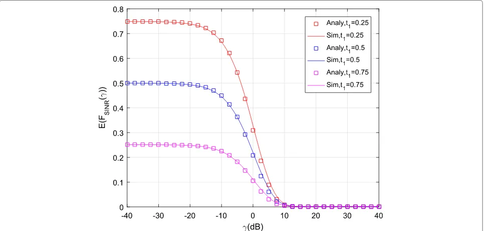
E!F¯SINR(γ ) "
=t1F¯SINR(γ )+(1−t1)F¯SINR(γ ) (40)
E!SEMT0 "
=t1SEMT0+(1−t1)SEMT0 (41) E!BRMT0
"
=t1BRMT0+(1−t1)BRMT0 (42)
where t1 denotes the duration of the first time slot, and
the entire time allocated for transmission is normalized to 1 for simplicity. This implies that the duration of the second time slot is 1−t1. The symbols with the “overline”
denote the performance metrics during the second time slots, where the MTs that are muted in the first time slot are the only ones allowed to transmit.
Since the network operation during the first time slot coincides with the IAM scheme that is studied in the previous sections, in this section, we analyze only the per-formance during the second time slot. In this case, we need to replaceAMTiwithAMTi, based on the notation in Table1.
7.1 General cell association criterion
We start introducing some enabling results to prove the main theorems.
Table 2SINR thresholds and SE values obtained from the LTE link-level simulator in [9,10]
iCQI 1 2 3 4 5 6 7 8 9 10 11 12 13 14 15
Proposition 7The probability that the typical MT is muted and is associated with tier j is
Pr
ProofSee AppendixC.
Lemma 5The probability density function (PDF) of the distance between the typical MT and its serving BS by con-ditioning on the eventXMT(j,m0)∩AMT0can be formulated as
(10), (45), and(46)respectively.
ProofThe Cumulative Distribution Function (CDF) of
the distance between the typical MT and its serving BS by conditioning on the MT being muted and onXMT(j,m)
0 is
obtained by using steps similar to AppendixA. The PDF is obtained from the CDF by computing the derivative.
Lemma 6Assume that the typical MT is associated with a BS of tier j. The Laplace transform of the (conditional) interference in time slot 2 can be formulated as follows:
LIM
is the PDF of the distance between the ith interfering MT and its serving BS for all the MTs,
χall(s,r)is defined as follows:
is defined as follows:
Pr
Theorem 3 The CCDF of the SINR of the typical MT in time slot 2 can be formulated as follows:
¯
7.2 Smallest path loss association
In this section, we study the smallest path loss cell asso-ciation criterion. In this case, the condition t(1) = t(2)
holds and simplified formulas can be obtained. Under the assumption that the path loss exponents of all the tiers of BSs are the same, in fact, multi-tier HCNs reduce to an equivalent single-tier cellular network of intensity# λ=
j∈Kλ
(j)[2].
Proposition 8The probability that the typical MT is muted can be formulated as follows:
PrAMT0
ProofThe proof is similar to that ofProposition7.
Corollary 3If = 1, PrAMT0
in(52)simplifies as follows:
ProofIt directly follows from52by setting = 1 and computing the integral.
Lemma 7The PDF of the distance between the typical MT and its serving BS is as follows:
fRMT0
Proof The proof is similar to that of Lemma 5. The
difference is that only the joint PDF of the distance of nearest and second nearest BSs needs to be used (see AppendixC).
Lemma 8Assume = 1. The Laplace transform of the aggregate interference can be formulated asLI(s) =
exp(βall(s)−β(s)), whereβ(s)is defined in Lemma4and system operates in the interference-aware regime (i0<p0). The CCDF of the SINR in time slot 2 can be formulated as follows:
Proof With the aid of the total probability theorem, we have: The proof follows by computing the two remaining expec-tations.
8 Numerical results and discussion
In this section, we validate the mathematical frameworks and findings derived in the previous sections with the aid of Monte Carlo simulations, as well as compare the IAM scheme against IAFPC and IUFPC schemes. The following setup compliant with LTE specifications is con-sidered. The bandwidth is equal to 10 MHz, which implies
bw = 9 MHz by excluding the guard bands. The noise
power spectral density is nthermal = − 174 dBm/Hz,
and the noise figure of the receiver is nF = 9 dB.
Both GCA and SPLA criteria are studied, and the asso-ciation weights are, unless otherwise stated, t(1)/t(2) =
t(1)/t(2) = 9 dB is related to a cell association based on
the average DL received power criterion, where the first tier of BSs (macro) has transmit power equal to 46 dBm and the second tier of BSs (small-cell) has transmit power equal to 37 dBm, which agrees with ([18], Annex A: Simu-lation Model). Other simuSimu-lation parameters are provided in Table 3. As far as Monte Carlo simulations are con-cerned, they are obtained by considering 104realizations of channels and network topologies. In all the figures, ana-lytical and Monte Carlo simulation results are represented with solid lines and markers, respectively.
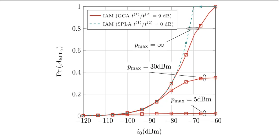
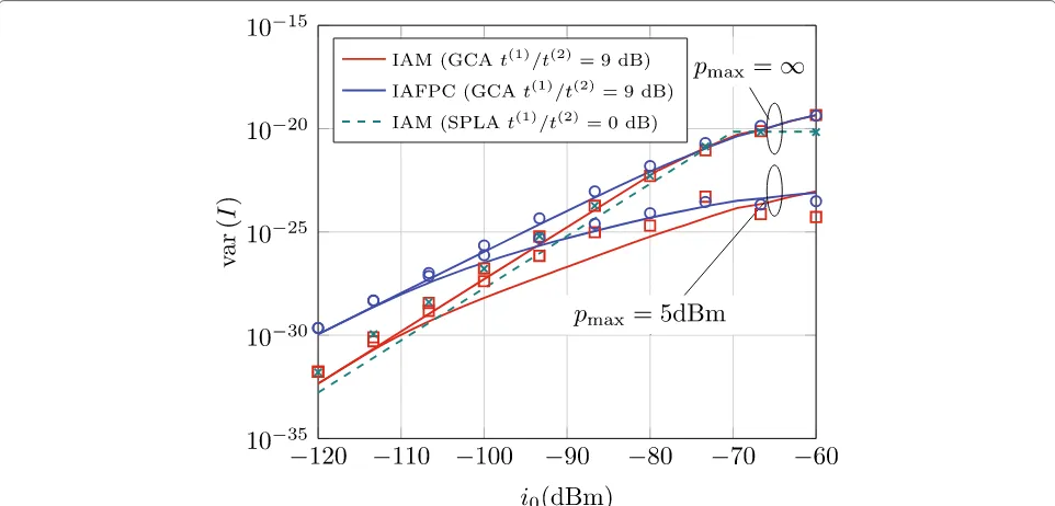
8.1 Average transmit power, probability of being active, mean, and variance of the interference
In this section, we analyze the average transmit power of the MTs, the probability that the typical MT is active, which provides information on the system fairness, and the mean and variance of the interference.
Figures 1, 2, 3, and 4 confirm the conclusions drawn inRemark1, i.e., the mathematical frameworks of aver-age transmit power and probability of being active are exact while those of mean and variance of the interfer-ence are approximations that exploitAssumption1. Such an assumption considers that the position of interfering MTs can be modeled as a conditionally thinned (i.e., homogeneous) PPP. The difference between such a non-homogeneous PPP, and the actual point process, which is on the other hand not tractable, explains also the differ-ence between simulation and analytical results in all the metrics that depend on the interference (SINR, SE, BR). The conclusions drawn in Remark 2 are confirmed as well: the mean and variance of the interference decrease by decreasingi0, which provide important advantages for
implementing AMC schemes.
In the figures, IAM and IAFPC are compared as well. We observe that IAM reduces the average transmit power and the mean and variance of the interference.
Consider the SPLA criterion, which is illustrated with dashed lines in the figures. We observe that the findings in Remark4are confirmed: the system is interference-aware and interference-uninterference-aware ifi0 < p0andi0 > p0,
respectively. As expected, the crossing point occurs at
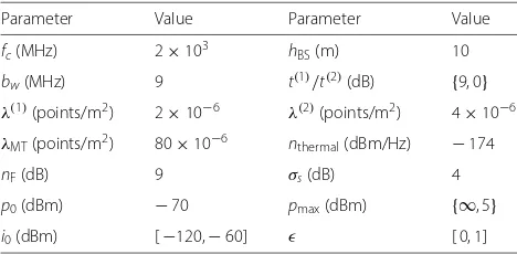
Table 3Simulation setup
Parameter Value Parameter Value
fc(MHz) 2×10³ hBS(m) 10
bw(MHz) 9 t(1)/t(2)(dB) {9, 0}
λ(1)(points/m2) 2×10⁻⁶ λ(2)(points/m2) 4×10⁻⁶ λMT(points/m2) 80×10−6 nthermal(dBm/Hz) −174
nF(dB) 9 σs(dB) 4
p0(dBm) −70 pmax(dBm) {∞, 5}
i0(dBm) [−120,−60] [ 0, 1]
p0 = − 70 dBm based on the simulation
parame-ters used. In addition, the scaling laws of average transmit power and average interference are in agreement with the findings inRemark7andRemark8.
All in all, the numerical illustrations reported in Figs.1, 2, 3, and 4 confirm all the conclusions and per-formance trends discussed in the previous sections and highlight the advantages of IAM.
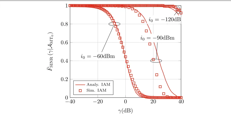
8.2 Complementary cumulative distribution function of the SINR
In this section, we analyze the coverage probability (CCDF of the SINR) of the active MTs. The results are illustrated in Figs.5and6for = 1 and =0.75, respectively, and by assumingpmax→ ∞.
In both figures, we observe a good agreement between mathematical frameworks and Monte Carlo simulations. In particular, the figures confirm, once again, that the coverage probability of IAM increases as i0 decreases.
In Fig. 5, for example, almost all the active MTs have a SINR greater than 20 dB if i0 = − 120 dBm. This
good SINR is obtained because IAM keeps under con-trol the interference by muting the MTs that create more interference. Based on Fig.2, in fact, we note that only a small fraction of the MTs are allowed to be active for
i0= −120 dBm. The active MTs, however, better exploit
the available bandwidth. Similar conclusions can be drawn for = 0.75 shown in Fig.6. The main difference is that, in this latter figure, IAM provides almost the same cover-age probability fori0 = − 60 dBm andi0 = − 90
dBm. The reason is that the MTs transmit with less power if = 0.75 and, thus, there is almost no difference between the two interference constraints. This brings to our attention that the design of the UL of HCNs requires to jointly optimizei0,p0,pmax, and, in order to identify
the desired operating regime that fulfills the requirements in terms of system fairness and interference mitigation. The proposed mathematical frameworks can be used to this end.
8.3 Spectral efficiency and binary rate
In this section, the average SE and average BR are ana-lyzed, as well as the IAFPC and IAM schemes are com-pared against each other for several system setups.
In Fig.7, the average SE of IAFPC and IAM schemes is analyzed and three conclusions can be drawn. By comparing the average SE of the IAPFC scheme (i.e., for AMC schemes) and on the Shannon formula, we note, as expected, that the latter formula provides optimistic esti-mates of the average SE. By comparing the average SE of the IAM scheme for typical (active and muted) MTs and active (only) MTs, we note a different performance trend as a function ofi0. As for the active MTs, the average SE
Fig. 1Average transmit power versusi0for IAM and IAFPC methods with=1,pmax→ ∞, andpmax = 5 dBm
other hand, the average SE decreases asi0decreases. This
is because the loweri0is the more MTs are turned off,
which on average, contributes to reduce the SE of the typ-ical MT. By comparing the average SE of IAPFC and IAM schemes, we evince that IAFPC outperforms IAM for all relevant values of the maximum interference constraint
i0, since all the MTs are active under the IAFPC scheme.
The average SE of the active MTs under the IAM scheme
is, however, much better than that of the IAFPC scheme, since the other-cell interference is reduced.
The SE, however, does not provide information on the amount of bandwidth that the scheduler allocates to each active MT.
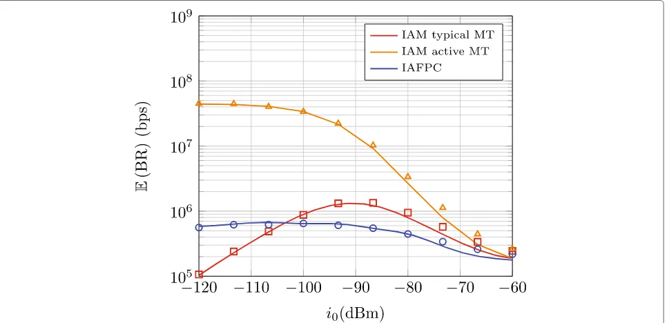
This trade-off is captured by the average BR, which is shown Fig.8. As far as the average BR is concerned, in particular, we note that IAFPC and IAM schemes provide
Fig. 3Mean of the interference versusi0for IAM and IAFPC methods with = 1,pmax→ ∞, andpmax = 5 dBm
opposite trends compared to those evinced from the anal-ysis of the average SE of the typical MT. More precisely, IAM provides a better average BR than IAFPC, and there exists an optimal value ofi0that maximizes it. This
opti-mal value ofi0 emerges if the typical MT is considered,
i.e., the MT may be either active or inactive. The figure, however, shows the average BR achieved only by the active MTs. In this case, we note that the MTs that satisfy both
power and interference constraints achieve a very high throughput due to the reduced level of interference that is generated in this case. In a nutshell, IAM outperforms IAFPC in terms of average BR because the available band-width is shared among fewer MTs (only those active), which results in a higher throughput for each of them. Even though some MTs may be turned off in IAM, this may not necessarily be considered as a downside from the
Fig. 5CCDF of the SINR for the typical MT conditioned on being active for IAM with = 1,t(1)/t(2) = 9 dB,pmax→ ∞, and i0 = {−120,−90,−60}dBm
user’s perspective: in high-mobility scenarios, for exam-ple, some MTs may prefer to be muted for some periods of time if their reward is achieving a higher throughput once they are allowed to transmit. In Fig.9, we study the impact of pmax for a given maximum interference
con-strainti0. We observe thatpmaxplays a critical role as well
and highly affects the average BR. This figure confirms, once again, that bothpmax andi0constraints need to be
appropriately optimized in order for IAM to outperform IAFPC.
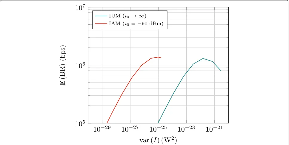
In Fig.10, we illustrate the potential of IAM of reduc-ing the variance of the interference compared with IUM,
Fig. 7Comparison of average SE of IAFPC and IAM for=1,t(1)/t(2)=9 dB andpmax→ ∞. As for IAFPC, the average SE based on the Shannon
formula is shown as well
while still guaranteeing the same average BR. As discussed in the previous sections, this is beneficial for implement-ing AMC schemes. The figure shows a four-order magni-tude reduction of the variance of the interference for the considered setup of parameters.
8.4 Impact of the association weights: on UL-DL decoupling
As shown in [2] and [5], optimizing the performance of HCNs for DL transmission does not necessarily results in optimizing their performance in the UL. Based on
Fig. 8Comparison of average BR of IAFPC and IAM for = 1,t(1)/t(2) = 9 dB, andpmax→ ∞. As for IAM, two cases are considered: the typical
Fig. 9Comparison of average BR of IAFPC and IAM for=1,t(1)/t(2)=9 dB andi0= −90 dBm
the GCA criterion, this implies that different cell associ-ation weights (i.e., a different ratio t(1)/t(2) for two-tier HCNs) may be needed in the DL and in the UL. However, this approach, which is referred to as UL-DL decoupling, introduces additional implementation challenges, which require the modification of the existing network architec-ture and control plane.
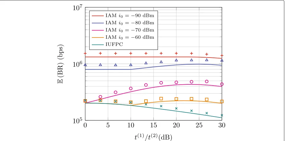
In this section, motivated by these considerations, we analyze and compare IAM, IAFPC, and IUFPC schemes as a function oft(1)/t(2). The setupt(1)/t(2) = 0 dB cor-responds to the SPLA criterion. Some numerical illustra-tions are provided in Figs.11and12, where the probability that the typical MT is active and the average BR are shown, respectively.
Fig. 11Probability the typical MT is active as a function oft(1)/t(2)for IUFPC (i0→ ∞) and IAM withi0 = {−90,−80,−70,−60}dBm. pmax→ ∞for both schemes
In Fig.12, in particular, we compare the average BR of IUFPC and IAM schemes. The figure highlights impor-tant differences between these two interference manage-ment schemes for improving the performance of the UL of HCNs. First of all, we note that the average BR of the IUFPC scheme decreases as the ratiot(1)/t(2) increases. More specifically, the best average BR is obtained if
the SPLA criterion is used, which is in agreement with previously published papers [16]. This originates from the fact that the largert(1)/t(2) is, the more MTs are asso-ciated with more distance BSs, which, due to the use of power control, results in increasing the interference in the UL. The performance trend is, on the other hand, different if the IAM scheme is used. In this case, there are
Fig. 12Average BR as a function oft(1)/t(2)for IUFPC (i
several values ofi0that provide a better average BR
com-pared with IUFPC. In addition, the average BR increases ast(1)/t(2)increases, since the excess interference that is generated under the IUFPC scheme is now kept under control by imposing the maximum interference constraint
i0. As observed in previous figures, Fig.11confirms that
this gain is obtained since more MTs are turned off. Figures11and12confirm the findings inRemark3and, in particular, the existence of an operating regime where the performance of IAM is independent of the associa-tion weights. Let us consider, for example, the setup for
i0 = − 60 dBm. In this case,i0>p0and hence,
accord-ing to Remark 3, the system is interference-unaware if t(1)/t(2) ∈[− 10,+ 10] dB. Figure 12, more
specifi-cally, confirms that IAM is interference-unaware since it provides the same average BR as IUFPC for t(1)/t(2) ∈
[− 10,+ 10] dB6. Similar conclusions can be drawn for other values ofi0, where different operating regimes can
be identified as predicted inRemark3. Ifi0 = −90 dBm,
in particular, theni0 <p0and the system is independent
of the cell association criterion fort(1)/t(2)∈[−20,+20], which is confirmed in Figs.11and12. It is worth men-tioning that the values oft(1)/t(2)for which the considered system model is cell association independent are usually adopted in practical engineering applications. In partic-ular, the authors of [2,19] have shown that the optimal cell association ratio that optimizes the DL is usually less than 20 dB. This is in agreement and compatible with the findings in Figs.11and12.
In view of the numerical results and theoretical insights derived in this work, it is possible to state the following arguments in favor of IAM:
1 Taking into account the periods where the typical MT is active and those where it is muted, the average BR is increased with IAM compared to IAFPC and IUFPC.
2 Thanks to mobility and shadowing, MTs are only muted for a given period of time.
3 Since the muted MTs do not transmit, their average transmitted power is reduced compared to IAFPC and IUFPC. This has been studied with Fig.1. 4 With IAM, there is a regime where the UL
performance is independent of cell association, which eases the joint design of UL and DL transmissions as it have been discussed above. 5 The IAM scheme can be further enhanced as
discussed in Section7. Some numerical illustrations are provided in the next section.
8.5 Hybrid scheme—complementary cumulative distribution function of the SINR
In this section, we analyze the coverage probability (CCDF of the SINR) of the hybrid scheme introduced in Section7.
The results are illustrated in Figs. 13, 14, and 15for
i0 = − 70,i0 = − 90, andi0 = − 120, respectively,
and by assuming = 1 andpmax→ ∞.
In these figures, we observe a good agreement between analytical frameworks and Monte Carlo simulations.
In Fig.13, it can be observed that the coverage prob-ability of the hybrid scheme increases as t1 increases.
In Fig. 14, it can be observed that the coverage prob-ability of the hybrid scheme decreases first and then increases as t1 increases. In Fig. 15, it can be observed
that coverage probability of the hybrid scheme decreases ast1decreases. As for highi0, these trends are obtained
because the coverage probability in time slot 1 is better than in time slot 2 for highi0since more MTs are active.
Then, increasingt1improves the coverage probability. As
for lowi0, the trend is opposite for similar reasons. The
comparison of these figures also shows that the coverage probability of the hybrid scheme decreases asi0increases
for small value of t1 because time slot 2 dominates the
performance. On the contrary, the coverage probability of the hybrid scheme increases as i0 increases for large
value oft1.
8.6 Hybrid scheme—spectral efficiency and binary rate In this section, the average SE and average BR are ana-lyzed.
In Fig. 16, the average SE of the hybrid system is reported. By comparing the average SE of the typi-cal MTs, we note a different performance trend as a function of i0 for different values of t1. If t1 = 1,
which is the IAM scheme, the average SE increases as
i0 increases as discussed in the previous sections. If t1 = 0, only the muted MTs transmit signals and the
average SE decreases as i0 increases. If, e.g., t1 = 0.5,
the average SE increases first and then decreases as i0
increases.
This result is reasonable because the lower i0 is the
fewer MTs transmit in time slot 1 and more MTs transmit in time slot 2, which on average, contributes to reduce the SE ift1 = 1 and to increase the SE ift1 = 0. As for the
hybrid scheme, the SE is somehow in between.
The average BR for different values of t1 is
illus-trated in Fig. 17. We note that the average BRs are quite similar if t1 = 0, while the gap increases if t1 = 1. We observe a quite large gap as a
func-tion of t1. This highlights that t1 should be carefully
allocated in order to fulfill system fairness and interfer-ence mitigation. The proposed mathematical frameworks can be used to optimize these competing performance metrics.
9 Conclusion
Fig. 13CCDF of the SINR of the hybrid scheme for the typical MT with=1,t(1)/t(2)=9 dB,pmax→ ∞andi0 = − 70 dBm
throughput of HCNs. With the aid of stochastic geome-try, we have developed a general mathematical approach for analyzing and optimizing its performance as a function of several system parameters. Simplified and insightful expressions of the throughput and other relevant per-formance indicators have been proposed for simplified but relevant case studies, such as in the presence of
channel inversion power control and equal cell association weights. Among the many performance trends that have been identified, we have proved that, while optimiz-ing the DL and the UL of HCNs necessitates, in gen-eral, to use different cell association weights, there exist some operating regimes where IAM is cell associa-tion independent. This is shown to simplify the design
Fig. 15CCDF of the SINR of the hybrid scheme for the typical MT with = 1,t(1)/t(2) = 9 dB,pmax→ ∞, andi0 = −120 dBm
of HCNs, since no changes in their control plane is needed compared with conventional cellular networks. The mathematical frameworks and findings have been substantiated against Monte Carlo simulations, as well as the achievable performance of IAM has been compared against other IAFPC and IUFPC schemes, by highlighting
several important trade-offs in terms of system fair-ness and system throughput. Finally, we have intro-duced a hybrid scheme that overcomes some fairness issues associated with the operating principle of the IAM scheme, and have highlighted important performance trade-offs.
![Table 2 SINR thresholds and SE values obtained from the LTE link-level simulator in [9, 10]](https://thumb-us.123doks.com/thumbv2/123dok_us/910141.1109967/12.595.57.541.690.734/table-sinr-thresholds-values-obtained-lte-level-simulator.webp)