R E S E A R C H
Open Access
Wideband UHF and SHF long-range
channel characterization
Edward Kassem
1, Jiri Blumenstein
1*, Ales Povalac
1, Josef Vychodil
1, Martin Pospisil
1, Roman Marsalek
1and Jiri Hruska
2Abstract
This paper presents an outdoor long-range (from 315 m up to 5.3 km) fixed channel campaign for both ultra high frequency and super high frequency bands with co-polarized horizontal and vertical antenna configurations. It investigates the channel characteristics of device to device communication scenarios underlaying the 5th generation networks by providing detailed research. Both line of sight and non-line of sight measurements in 1.3 GHz and 5.8 GHz frequency bands with bandwidth up to 600 MHz were conducted. The path loss, root mean square delay spread, coherence bandwidth, and channel frequency response variation are characterized. We observed that the variation is negligible in microcell line of sight environment for both above mentioned frequencies, whereas it significantly increases with frequency in different macrocell non-line of sight environments. The distance dependency of path loss was also derived. It was observed that the root mean square delay spread decreases with frequency for both line of sight microcell and non-line of sight macrocell measurements. A dependency between the root mean square delay spread and transmitter-receiver distance in non-line of sight environments was also captured. The relation between the coherence bandwidth and the root mean square delay spread was depicted. It demonstrates an exponential function in all considered channel combinations.
Keywords: Channel model, Device to device, Line of sight, Non-line of sight, Super high frequency, Ultra high frequency
1 Introduction
Device to device communication [1, 2] is an important technology which enables data flow not only between humans but also between machines without human inter-vention. It can be used underlying the available cel-lular networks. The 5th generation system technology, 3rd Generation Partnership Project Release 15, will have to support high performance in spectral efficiency and throughput measurements. The 5th generation network is one of the most suitable environments for device to device communication since it is an IP-based network that enables to control any connected devices using inter-net protocols. Moreover, it is able to send large amounts of data with a high rate and low latency and support a large amount of connected devices. It is a good solution to reduce the eNB traffic load and the end to end delay. In
*Correspondence:[email protected]
1Department of Radio electronics, Brno University of Technology, Technicka 12, Brno, Czech Republic
Full list of author information is available at the end of the article
order to develop a reliable wireless device to device com-munication network [3,4], an accurate description of the wireless channel impulse response measurements should be presented. The channel impulse response describes spreading, echoing, multipath propagation, and Doppler effects that occur when an impulse is sent between the transmitter and the receiver. Knowledge of the channel impulse response characteristics enables system designers to ensure that inter symbol interference does not dominate and hence lead to an excessive irreducible bit error ratio [5].
1.1 Literature review
As mentioned above, propagation measurements are nec-essary for creating statistical channel models that support the development of new standards and technologies for wireless communications systems. Channel models that predict signal strength and multipath time delays are required for a proper system design. There have been a number of studies for channel sounding using different input signals over the past 10 years.
As a sample of typical work, there is a paper which studied the frequency dependence of the channel charac-teristics at the 2–4 GHz frequency band [6]. Line of sight and obstructed line of sight scenarios were considered. Angle of arrival and delay of arrival of the main paths were investigated. A rich multipath environment was observed, with intensive path components existence in both angle and delay domains.
Outdoor measurements were conducted in an open-area test site at the National Metrology Institute of Germany [7], to study the scattering effects of a traffic sign on vehi-cles moving along the road. The outputs are analytical modeling, simulation, measurement, and implementation of the bi-static radar cross section of the traffic signs.
A paper on outdoor sounding [8] highlighted the prop-agation path loss models for 5th generation urban micro and macro cellular scenarios. It compares the alpha-beta-gamma and the close-in free space reference dis-tance models. A wide range of frequencies 2–73.5 GHz over 5–1429 m distances were used. The output showed very comparable modeling performance between close-in and alpha-beta-gamma models. The close-close-in model offers simplicity and a conservative non-line of sight path loss estimate at large distances, whereas the alpha-beta-gamma model is more complex and offers a fraction of a decibel smaller shadow, less loss near the transmitter, and more loss far from transmitter.
Another paper [9] described the achieved results for line of sight and non-line of sight measurements between the User Equipment and the base station in Nanjing Road, Shanghai. The received signals were 20 MHz band-width with 2.1376 GHz carrier frequency. The delays and the complex attenuations of multipath components have been estimated by applying the space-alternating gener-alized expectation-maximization algorithm. The distance between transmitter and receiver in line of sight/non-line of sight scenarios, the life-distance of the sight/non-line of sight channel, the power variation at line of sight to non-line of sight transition, and the transition duration were extracted.
The authors in [10] presented a sounding system that uses an orthogonal frequency division multiplexing signal at 5.6 GHz with 200 MHz bandwidth. The power delay profiles and the excess delay were presented.
An open-pit mine campaign performed a 25-MHz wide frequency band sounding immediately below the unli-censed 2.4-GHz ISM band [11]. A continuously repeat-ing maximum-length or m-sequence with K = 2047 sequence length was adopted as a transmitted signal. It was transmitted at a rate of 25 MS/s. Four measure-ment realizations of the impulse response with different transmitter-receiver separations that vary between 425– 1670 m were recorded. The calculated delay spread of the channel was often more than 10μs.
A channel measurement campaign was conducted to study the frequency dependence of the propagation chan-nel for a wide range of frequencies 3–18 GHz [12]. Urban macro and micro cellular environments were covered. The root mean square delay spreads, coherence bandwidth, path loss, shadow fading, and Ricean factor were charac-terized. It is mentioned that the path loss exponents vary significantly with frequency (from 1.8 to 2 dB in a line of sight environment and from 2.71 to 4.34 dB in non-line of sight). Shadow fading and the Ricean factor increase with frequency, whereas the root mean square delay spread val-ues decrease with frequency in a line of sight environment. However, the root mean square delay spread in a non-line of sight environment and the coherence bandwidth values in both line of sight and non-line of sight environments do not show significant changes.
An outdoor wideband channel sounding at 2.4 GHz is described in [13]. The distance between the transmitter and the receiver varied from 50 to 150 m. The distance-power gradient is 2.532, path loss (with 9 dB standard deviation), small-scale or multipath fading (with 5 dB standard deviation) are reported. The maximum observed multipath fade is 28 dB.
Another campaign was conducted in Seoul [14]. The measurements were done using a wideband channel sounder at 3.7 GHz with a 100 MHz bandwidth. Both line of sight and non-line of sight environments are investi-gated. The output was presented as a spatial correlation coefficient of low-height links in an urban environment.
A wideband propagation channel at 2.45 and 5.2 GHz was presented in [15]. Channel characteristics as power delay profile, the mean delay, and the delay spread were studied. It was mentioned that the parame-ters are frequency-independent, whereas the higher frequency signal shows considerably larger path loss than the lower one. Both the correlator-based and recursive Bayesian filter-based ranging estimators were evaluated; both of them provide better performances at 2.45 GHz compared with 5.2 GHz. The perfor-mance difference increases with decreasing the received power.
Measurement campaign [17] at the center frequency of 2.35 GHz with 50 MHz bandwidth was conducted in order to evaluate the performance in an outdoor propa-gation environment. Signal to noise ratio, spatial diversity, and capacity of different transmission schemes (direct transmission, amplify and forward, and decode and for-ward relaying) were investigated. Both line of sight and non-line of sight scenarios were involved. The results were depicted in terms of signal to noise ratio, spatial diversity, and capacity. Both amplify and forward, and decode and forward schemes improve the Signal to Noise Ratio, whereas direct transmission improves the capacity in small distances of a line of sight environment. However, by increasing transmitter-receiver distance, the capacity provided by the decode and forward exceeds that provided by the direct transmission. The spatial diversity was also significantly improved by applying the decode and for-ward scheme. Most of the abovementioned papers depict indoor channels or even outdoor channels but only up to 2 km and with only vertical co-polarization. There-fore, we filled these gaps by considering both line of sight and macro non-line of sight scenarios over 1.3 GHz and 5.8 GHz frequencies with longer distances 2.089 km, 4.11 km, and 5.429 km and both vertical and horizon-tal co-polarization dependence of multipath propagation channel measurements.
1.2 Contribution of the paper
We analyzed the channel frequency response variation, the path loss, the root mean square delay spread, and the coherence bandwidth with all above mentioned scenar-ios. Our achieved results expand the achieved results in [18] which were performed in an indoor environment. The main contributions of this paper are described in the following few points:
• Test the ability of deploying a device to device communication underlay 5th generation network in a wideband long-range channel for both ultra high frequency and super high frequency bands as a part of 5th
generation new radio frequency bands allocation [19]
• For a microcell line of sight environment (with 315 m distance), we provided the channel frequency response variation, the path loss, and the root mean square delay spread distribution in the case of vertical and horizontal polarizations for both 1.3 GHz and 5.8 GHz center frequencies.
• For macrocell non-line of sight environments (with 2.089, 4.11, and 5.429 km distances), in additional of all previous mentioned parameters, distance dependence of the path loss and the root mean square delay spread are analyzed. The root mean square delay spread dependence of the coherence bandwidth is also investigated.
This paper is organized as follows. The “Materials and methods” section describes the channel measurement campaign of outdoor long-range environments and the sounder systems for ultra high frequency and super high frequency bands. The data processing procedure and channel characteristics calculation are also depicted. In the “Results and discussion” section, the channel mea-surement results are captured for line of sight and non-line of sight outdoor environments with different polar-ization combinations. Based on channel measurement results, the root mean square delay spread, the path loss, the channel frequency response variation, and the coher-ence bandwidth are analyzed. The last section concludes the paper.
2 Materials and methods
2.1 Measurement environments and setup
Our measurements were conducted in the South Moravian region, Czech Republic. Two types of setups: microcell and macrocell were considered.
In the microcell setup, the TX1 was placed on a small hill near the Faculty of Electrical Engineering and Communication building, Brno University of Technology (BUT) and mounted on a mast of 10 m height, whereas the receiver was allocated on the rooftop of the building (19-m height). The distance between the transmitter and the receiver for route R1 is 315 m. Both the transmitter and the receiver are surrounded by a rich scattering environment which consists of buildings, parked cars, moving cars, and people. However, because of the highly mounted anten-nas above the ground, line of sight measurements were realized.
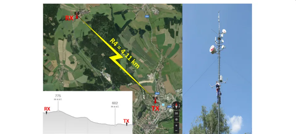
In the macrocell setup, three different non-line of sight routes (R2, R3, R4) were tested. On the first two routes (R2, R3), the receiver was placed on the rooftop of the Faculty of Electrical Engineering and Communication building. The transmitter was allocated 2.089 km from the receiver (8-m height) for the R2 route, and 5.429 km from the receiver (3 m height) in the case of the R3 route. For the fourth route, R4, both the transmitter and the receiver were allocated in a rural area where the transmitter was surrounded with different building heights (up to 12-m height) and placed on the rooftop of the Racom company building (12-m height) mounted on a mast of 5-m height. The receiver was mounted on a mast of 19-m height in a pure rural area. Examples of transmitting antennas in the case of R2 and R3 and receiving antenna with their surrounding environments are presented on the left-hand side, the right-hand side, and the center of Fig.1, respec-tively. The mast of the received antenna of the fourth route, R4, is captured on the right-hand side of Fig.2.
Fig. 1Measurement locations for R1, R2, and R3 routes. Line of sight route R1 = 315 m and non-line of sight route R2 = 2.089 km with super high frequency band TX2 position on the left-hand side, R3= 5.429 km with ultra high frequency band TX3 position on the right-hand side and the position of the sector receiver antenna used for the super high frequency signal of TX2-RX measurements. Map source: Google.com, Mapy.cz
implemented. These sounders together with MATLAB and LabVIEW programs were used for channel evaluation up to 120 MHz and 600 MHz bandwidths for both 1.3 and 5.8 GHz, respectively.
The basis of the transmitting station is a programmable radio frequency generator (R&S SMU200A vector signal generator). The generated signal was filtered using a band
pass filter, amplified by a power amplifier, and directed to the directional antenna transmitter using a circular con-nector. The amplifier module for the ultra high frequency band (MD220L-1296-48V) was modified to be used as a linear amplifier class A. However, the super high fre-quency band transmitter uses Hittite HMC408LP3 and DG0VE PA6-1-8W amplifying modules. The generated
ultra high frequency (1.3 GHz) signal was transmitted using 35-element Yagi Tonna antenna 20365 with 20 dBi of gain. The super high frequency (5.8 GHz) signal was transmitted by a parabolic RD-5G30-LW RocketDish with a gain equaling 30 dBi.
The receiver consists of a directional antenna, low-noise amplifier, and signal analyzer (National Instruments PXIe-5665) with three basic modules: PXIe-5653 RF synthe-sizer, PXIe-5605 downconverter, and PXIe-5622 150 MS/s 16-bit digitizer. The ultra high frequency and super high frequency signals were received by 35-element Yagi Tonna antenna 20365 (20 dBi gain) and sector antenna AM-V5G-Ti (21 dBi gain), respectively.
The developed software in LabVIEW environment for National Instruments PXIe-5665 was used for record-ing and processrecord-ing the raw data received by the channel sounder. This software is able to record up to 600 MHz of bandwidth via stepped re-tuning by 50 MHz blocks with the ability to be synchronized with the transmitted signal. In order to save the achieved data with 50 MHz instance bandwidth and 16-bits precision, a redundant array of inexpensive disks with capacity of 12 TB and 16-bit dynamic range was used. MATLAB was also used for final data processing. Our in-house developed channel sounder operates with frequency modulated continuous wave, i.e., as a sounding sequence; we utilize frequency modulation chirps with a maximal measurement speed of 40 MHz/ms. Figure 3 depicts the schematics of the sounder for ultra high frequency (white blocks) and super high frequency (gray blocks) bands, whereas the charac-teristics (E and H planes) of both parabolic and sector antennas for vertical and horizontal co-polarizations are captured in Fig.4.
2.2 Data processing 2.2.1 Channel response
The radio channel is commonly characterized by scat-tering, attenuation, reflection, refraction, and fading [20]. In both the wired and wireless communications, the Additive White Gaussian Noise channel is assumed as a basic channel model. More advanced models includ-ing fadinclud-ing effects, e.g. the International Telecommunica-tion Union path loss models like Flat Rayleigh, Pedes-trian (Ped), and Vehicular (Veh) [21]. The Flat Rayleigh fading channel has a constant attenuation factor during the subframe time and the whole allocated bandwidth. Other two models define two different test environ-ments: outdoor to indoor pedestrian and vehicular well-established channel models used for research purposes in mobile communication systems. The impulse responseh of the multipath channel can be calculated according to Eq. (1), where βw, τw, and ϕw represent the amplitude, arrival time, and phase that characterize the Np
num-ber of individual paths between the transmitter and the receiver [21].
h(t,τ)=
Np
w=1
βw(t)·δ (t−τw(t))e−jϕw(t) (1)
The frequency response can be measured directly by collecting the measurements of thes21scattering
parame-ter of a radio channel in the frequency domain. It can also be calculated by applying the Fourier transformation on the time domain measurements expressed in Eq. (1). The result could be given by Eq. (2) [22].
Fig. 4Parabolic and sector antennas rectangular radiation. Both E and H planes in the case of vertical and horizontal co-polarizations are captured
H(f,t)=
∞
−∞h(t,τ)·e −jωτdτ
=
Np
w=1
βw(t)e−jϕw(t)e−jωτw(t)
(2)
In a slowly time-varying channel, the multipath parame-ters of the channel remain constant during fractions of the coherence time of the channel; so the frequency response can be presented in Eq. (3).
H(f)=H(f, 0)=
Np
w=1
βwe−jϕwe−jωτw (3)
In practice, however, the measurement systems are band-limited. Therefore, the frequency response is defined in Eq. (4).
H(f)=H(f, 0)=W(f)·
Np
w=1
βwe−jϕwe−jωτw (4)
where W(f) represents the frequency domain RF filter characteristics in the frequency domain.
2.2.2 Path loss
The generalized form of the path loss model can be con-structed from path loss offset PLoffset, the distance d
between transmitter and receiver, the reference distance d0, and the random shadowing effectχσ which is
calcu-lated as the deviation of the measured path loss from the linear model [12].
PL(d)=PLoffset+10n·log
d d0
+χσ (5)
wherenis a path loss exponent andd0 =100 m for long
outdoor distances [20].
2.2.3 Root mean square delay spread
fading channels and a guideline to design a wireless trans-mission system. Ifτwis the channel delay ofwth path and P(τw)is its power, then the root mean square delay spread can be formulated in Eq. (6).
Coherence bandwidth is a statistical measure of range of frequencies over which the channel can be considered as a flat channel. In other words, coherence bandwidth is the range of frequencies over which two frequency compo-nents have a strong potential for amplitude correlation. In the case where the coherence bandwidth is defined as a bandwidth with correlation of 0.5 or above, it can be cal-culated using the frequency correlation function depicted in Eq. (10) [12].
S( f)∼=
∞ −∞H(f)H
∗(f + f).df (9)
H(f)is the complex transfer function of the channel, f is frequency shift and * denotes the complex conjugate.
Bc,0.5≈min
2.2.5 Channel frequency response variation
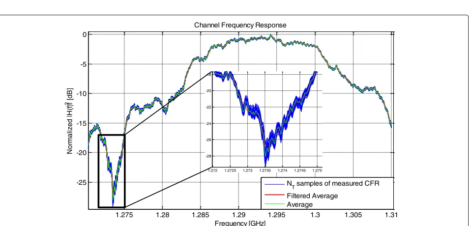
Let us consider that Hs(fk), k = 1, 2,· · ·NF, s = 1, 2,· · ·,NT is the wideband channel frequency response at specific time for a specific frequency. Figure5depicts a sample (NT = 200) of normalized channel frequency response in dB wheref1 = 1.2702 GHz,f2 = 1.31 GHz,
therefore f = f2−f1 = 39.758 MHz, andNF = 1554. The influence of variation and small-scale fading can be removed by averaging consecutiveNT channel frequency response characteristics [23] according to Eq. (11).
H(fk)2=
However, as is mentioned in [24], averaging keeps some small-scale fluctuations in the frequency domain; there-fore, the median filter is applied. The median filter is a non-linear filter used to discard the noise from the signal. The main idea is to run through the whole signal and calculate the median of each window [25]. Note that in order to get a well-filtered signal, a proper window size of median filter (that keeps the deep fades effect) should be chosen. In our research, the window size will depend primarily on the deep fades where the signal strength can drop for more than 15 dB. Therefore, the window size of 10 is chosen as the average frequency distance of the deep
1.275 1.28 1.285 1.29 1.295 1.3 1.305 1.31 -25
NT samples of measured CFR Filtered Average
Average
1.272 1.2725 1.273 1.2735 1.274 1.2745 1.275 -28
fades. Finally, the channel frequency response variation is obtained through subtracting the filtered average channel frequency response from the measured channel frequency response.
3 Results and discussion 3.1 Path loss
Figure6presents the cumulative distribution function of the path loss for a line of sight environment. The cumu-lative probability of path loss values fit well with the nor-mal distribution withμmean andσ standard deviation parameters.
The path loss values of the R1 line of sight route are in the range of 87.6–88.5 dB with a mean value 88.1 dB and standard deviation 0.22 dB for 1.3 GHz with horizontal co-polarization, 88.2–89.9 dB with a mean value 89.04 dB and standard deviation 0.33 dB for 1.3 GHz with vertical co-polarization, 114.9–116.1 dB with a mean value 115.49 dB and standard deviation 0.23 dB for 5.8 GHz horizontal co-polarization, and 116.5–117.9 dB with a mean value 117.1 dB and standard deviation 0.24 dB for 5.8 GHz with vertical co-polarization.
The distribution shape is also depicted in Fig. 6 and presented in black, blue, magenta, and cyan colors for ultra high frequency horizontal co-polarization, ultra high
frequency vertical co-polarization, super high frequency horizontal co-polarization, and super high frequency ver-tical co-polarization, respectively. The shape can provide useful information about the density of the calculated path loss. It can be observed that in the case of both 1.3 and 5.8 GHz, the path loss for vertical co-polarization exceeds the path loss of the horizontal one. This small difference (1– 2 dB) is explained by the effect of suppression which can influence either the vertical or the horizontal polarization. That depends on the distance between transmitter and receiver, their heights, and the type of ground [26,27]. It is also clear that the path loss increases with frequency as the higher frequencies tend to suffer greater signal absorp-tion and scattering. The same characteristics are observed in [6,8,20] higher frequencies tend to suffer greater signal absorption.
Figure7presents the measured path loss for 1.3 GHz sounding system in the case of horizontal and vertical co-polarizations. Black circles represent the measured path loss values for horizontally transmitted and received signals, whereas blue circles represent the measured path loss values for vertically transmitted and received signals. The best line fit have been produced using a MATLAB function with path loss exponents equal to 3.9 and 3.7 for horizontal and vertical polarization cases, respectively. These results are comparable with the results specified in [8], where the path loss exponent value for distances up to 1.4 km varies between 2.9 and 3.1 for 2 GHz
10−1 100 101 60
80 100 120 140 160 180
Distance [km]
Path loss [dB]
UHF Measured path loss for horizontal pol. n=3.9, PLoffset=81.1 dB
Measured path loss for vertical pol. n=3.7, PL
offset=89.9 dB
n=2 n=5
n=4
n=3
Fig. 7The measured path loss for 1.3 GHz center frequency of the outdoor non-line of sight environment. The black and blue circles represent the measured non-line of sight path loss values for horizontal and vertical co-polarization, respectively
frequency. The path loss exponent value was also captured in an urban environment [16] for 800 MHz frequency and reached the value ofn=3.3.
Figure8depicts the measured path loss for a 5.8-GHz sounding system in the case of horizontal and vertical co-polarizations, represented by black and blue circles, respectively. The best line fit has been produced using a MATLAB function with path loss exponentsn equal to 4.6 and 4.1 for horizontal and vertical polarization cases, respectively. These values can be compared with val-ues achieved in [12], for frequencies 3–6 GHz where the path loss exponents between 3.92 and 4.7 were achieved. According to outdoor measurements presented in [28], the path loss exponent value changes fromnequal to 2 tonequal to 4 at the breakpoints distance near 2.85 km.
The dashed gray lines represent the theoretical path loss model in the case of different exponents. Note that the path loss exponent represents the slope of the path loss line, whereasPLoffset = PLF + PLNLOS where PLF and PLNLOS are free space path loss and the path loss offset
due to non-line of sight environment effects. More infor-mation about the path loss values for different line of sight and non-line of sight scenarios are listed in Table1.
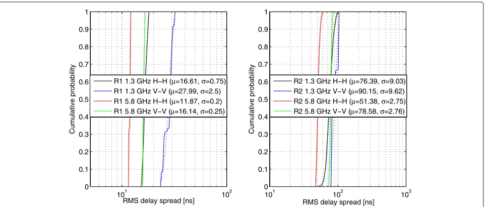
3.2 Root mean square delay spread
Figures 9 and 10 display the cumulative probability of the root mean square delay spread for the line of sight environment presented as R1 route and 2.089, 5.429, and 4.11 km non-line of sight environments presented as R2, R3, and R4 routes, respectively. The root mean square
10−1 100 101
80 100 120 140 160 180 200
Distance [km]
Path loss [dB]
SHF Measured path loss for horizontal pol. n=4.6, PLoffset=106.2 dB
Measured path loss for vertical pol. n=4.1, PL
offset=110.6 dB
n=2 n=5
n=3 n=4
Table 1The path loss mean, standard deviation, minimum, and maximum values for different frequencies and co-polarizations in both line of sight and non-line of sight environments
Path loss
Route Env. Freq. Pol. μ[dB] σ[dB] Min [dB] Max [dB]
R1 LOS
1.3 GHz H-H 88.1 0.22 87.6 88.5
V-V 89.04 0.33 88.2 89.9
5.8 GHz H-H 115.49 0.23 114.9 116.1
V-V 117.1 0.24 116.5 117.9
R2
NLOS
1.3 GHz H-H 130.84 0.37 129.77 132.31 V-V 137.54 0.62 136.74 138.39
5.8 GHz H-H 162.34 1.92 160.5 165.13 V-V 163.93 0.421 163.24 164.51
R3
1.3 GHz H-H 144.6 0.72 143.37 146.54 V-V 150.48 0.64 148.89 152.92
5.8 GHz H-H 184.48 2.88 179.68 189.86 V-V 180.95 0.38 180.08 181.76
R4
1.3 GHz H-H 145.61 1.46 143.55 147.54 V-V 149.9 0.44 149.23 150.67
5.8 GHz H-H 183.34 1.33 180.41 187.17 V-V 180.55 0.56 178.89 181.08
delay spread values for all routes and frequencies fit well with the normal distribution withμmean andσstandard deviation parameters.
It can be distinguished that the R1 line of sight route offers smaller root mean square delay spread compared with all plotted root mean square values for non-line
of sight environments in both 1.3 and 5.8 GHz. This behavior is expected. On the one hand, it can be due to a very strong line of sight component compared with the reflected or scattered path, leading to lower root mean square delay spread. On the other hand, in the case of a non-line of sight environment, the transmitted signal is blocked or severely attenuated causing mul-tipath to arrive at the receiver over a large propaga-tion time interval. Similar characteristics are observed in [12,29].
The wideband root mean square delay spread for the R1 route is in the range of 15.11–18.42 ns for 1.3 GHz with horizontal co-polarization, 23.18–32.58 ns for 1.3 GHz with vertical co-polarization, 11.53–12.21 ns for 5.8 GHz horizontal co-polarization, and 15.82– 16.62 ns for 5.8 GHz with vertical co-polarization.
It can be seen from Fig. 9 that in the case of the first route R1 line of sight, the higher frequency pro-vides smaller mean root mean square delay spread in both horizontal and vertical polarization settings. This behav-ior was also mentioned in [12, 30]. It is also clear that in the case of both ultra high frequency and super high frequency frequencies, the vertical co-polarization shows higher mean root mean square delay than horizontal co-polarization.
For the R2 route, the root mean square delay spread is in the range of 52.99–99.70 ns for 1.3 GHz with horizontal co-polarization, 77.44–104.82 ns for 1.3 GHz with vertical polarization, 46.43–60.67 ns for 5.8 GHz horizontal co-polarization, and 72.15–87.63 ns for 5.8 GHz with vertical co-polarization.
RMS delay spread [ns]
Cumulative probability
RMS delay spread [ns]
Cumulative probability
Fig. 9R1 and R2 root mean square delay spread. Cumulative Distribution Function of the root mean square delay spread in [ns] for different frequencies and both horizontal and vertical co-polarizations of the first and second measurement routes (R1 and R2) in line of sight and non-line of sight scenarios, respectively. The colored dotted lines represent the Normal distribution of the corresponding frequency and polarization
101 102 103
RMS delay spread [ns]
Cumulative probability
RMS delay spread [ns]
Cumulative probability
Fig. 10R3 and R4 root mean square delay spread. Cumulative distribution function of root mean square delay spread in [ns] for different
frequencies and both horizontal and vertical co-polarizations captured for the third and fourth measurement routes (R3 and R4). The colored dotted lines represent the normal distribution of the corresponding frequency and polarization combinations
In the case of the R3 route, the root mean square delay spread is in the range of 95.21–215.39 ns for 1.3 GHz with horizontal co-polarization, 137.24–151.27 ns for 1.3 GHz with vertical co-polarization, 157.7–189.54 ns for 5.8 GHz horizontal co-polarization, and 163.33–176.58 ns for 5.8 GHz with vertical co-polarization. For the R4 route, it is in the range of 66.85–119.73 ns for 1.3 GHz with hor-izontal co-polarization, 78.73–147.76 ns for 1.3 GHz with vertical co-polarization, 44.12–89.91 ns for 5.8 GHz hor-izontal co-polarization, and 70.44–119.11 ns for 5.8 GHz with vertical co-polarization. It can be observed that the horizontal co-polarization shows smaller mean root mean square delay spread than the vertical co-polarization for 1.3 and 5.8 GHz. However, the third route, R3, shows dif-ferent characteristics. This can be due to the building’s metal roof between the transmitter and the receiver, that cause depolarization. Table2combines all needed infor-mation about the root mean square delay spread values.
The effect of transmitter-receiver distance on the mean values of root mean square delay spread is also investi-gated. The mean root mean square delay spread values increase with the increasing distance between the trans-mitter and the receiver. A similar trend is observed in [31]. The relation between the mean root mean square delay spread and the distance can be fitted with linear mode
στUHF,H =20d+27 for ultra high frequency with horizon-tal co-polarization,στUHF,V =15d+55 for ultra high fre-quency with vertical co-polarization,στSHF,H =34d−33 for super high frequency with horizontal co-polarization, and στSHF,V = 25d + 15 for super high frequency with vertical co-polarization, where d is the distance
between the transmitter and the receiver in kilometers. This characteristic is comparable with results published in [32,33].
From these functions, it can be noticed that the line slope of the root mean square delay spread of super high
Table 2The mean, standard deviation, minimum, and maximum
values of root mean square delay spread for different frequencies and co-polarizations in both line of sight and non-line of sight environments
RMS delay
Route Env. Freq. Pol. μ[ns] σ[ns] Min [ns] Max [ns]
R1 LOS
1.3 GHz H-H 16.61 0.75 15.11 18.42
V-V 27.99 2.50 23.18 32.58
5.8 GHz H-H 11.87 0.20 11.53 12.21
V-V 16.14 0.25 15.82 16.62
R2
NLOS
1.3 GHz H-H 76.39 9.03 52.99 99.70
V-V 90.15 9.62 77.44 104.82
5.8 GHz H-H 51.38 2.75 46.43 60.67
V-V 78.58 2.76 72.15 87.63
R3
1.3 GHz H-H 148.19 35.69 95.21 215.39 V-V 143.40 4.07 137.24 151.27
5.8 GHz H-H 173.96 3.95 157.70 189.54 V-V 168.32 1.48 163.33 176.58
R4
1.3 GHz H-H 91.67 10.67 66.85 119.73 V-V 109.81 18.05 78.73 147.76
5.8 GHz H-H 67.25 12.70 44.12 89.91
frequency frequencies greater than the line slope of root mean square delay spread of ultra high frequency frequen-cies. Therefore, the mean root mean square delay spread for super high frequency frequencies more extremely increases compared with the mean root mean square delay spread of ultra high frequency frequencies. The same characteristics were captured in the case of com-paring horizontal and vertical co-polarization where the horizontally polarized signal is more sensitive to distance changes. All above mentioned properties are depicted in Fig.11.
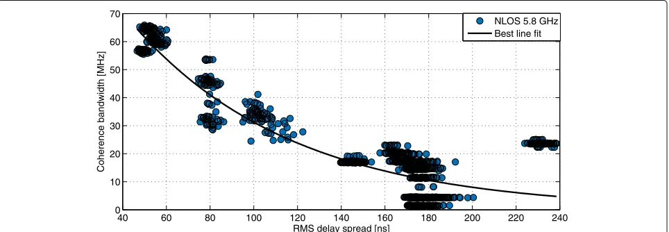
3.3 Coherence bandwidth
Figure 12 depicts the root mean square delay spread dependency of the coherence bandwidth in 1.3 GHz non-line of sight environments where the coherence band-width in MHz and the root mean square delay spread in ns. This relation is fitted with an exponential model Bc,0.5 = 18.34· e−0.002στ.
Figure13depicts root mean square delay spread depen-dency of the coherence bandwidth in 5.8 GHz non-line of sight environments where the coherence bandwidth is in megahertz and the root mean square delay spread is in nanoseconds. The measurements represented by blue circles, which were achieved from R2, R3, R4 route mea-surements, fit with the exponential modelBc,0.5 =121.5·
e−0.014στ. A similar relation was observed in [34,35].
3.4 Channel frequency response variation
Figure14depicts the cumulative probability of the mea-sured wideband channel frequency response variation for different routes (R1, R2, R3, R4) of 1.3 GHz center fre-quency and horizontal and vertical co-polarizations. It can be observed that the channel frequency response vari-ation values fit well with the Normal distribution which is plotted as a dotted curve colored according to a par-ticular route. The channel frequency response variations have mean values of 0.044, 0.25, 0.288, and 0.182 dB and
standard deviation of 0.036, 0.291, 0.403, and 0.196 dB in the case of horizontal co-polarization, whereas the mean values of 0.06, 0.127, 0.377, and 0.295 dB and standard deviation of 0.078, 0.172, 0.537, and 0.289 dB in the case of vertical co-polarization. It can be noticed that the chan-nel frequency response variations have the smallest mean and standard deviation values in the case of the R1 route which corresponds to the line of sight scenario.
Figure 15 presents the cumulative probability of the measured wideband channel frequency response variation for different routes (R1, R2, R3, R4) of 5.8 GHz center frequency and horizontal and vertical co-polarizations. It can be seen that the channel frequency response variation values also fit well with the Normal distribution which is plotted as a dotted curve colored according to a particu-lar route. The channel frequency response variations have mean values of 0.041, 3.083, 1.246, and 2.296 dB and stan-dard deviation of 0.119, 2.902, 1.686, and 2.3 dB in the case of horizontal co-polarization, whereas the mean values of 0.044, 3.48, 1.621, and 1.491 dB and standard deviation of 0.119, 2.952, 1.621, and 1.478 dB in the case of verti-cal co-polarization. The same feature of lowest mean and standard deviation values appears for the first route R1 which represents the line of sight scenario.
It is also clear from Figs.14and15that the channel fre-quency response variations increase with frefre-quency. This merit becomes more visible in the case of the non-line of sight scenario. The second route R2 shows the highest channel frequency response variation due to higher fre-quency signals which tend to scatter more than the lower ones. These scatter objects can be moving people and cars.
4 Conclusion
In this paper, a device to device outdoor long-range com-munication channel was utilized for a measurement cam-paign. Both ultra high frequency and super high frequency channels were sounded using Yagi Tonna antennas as a
2 3 4 5 6
50 100 150
Distance [km]
RMS delay spread [ns]
1.3 GHz signal
2 3 4 5 6
50 100 150
Distance [km]
RMS delay spread [ns]
5.8 GHz signal Horizontal co−polarization Vertical co−polarization Horizontal co−polarization
Vertical co−polarization
50 100 150 200 250 300 350 6
8 10 12 14 16 18 20
RMS delay spread [ns]
Coherence Bandwidth [MHz]
NLOS 1.3 GHz signal
NLOS 1.3 GHz Best line fit
Fig. 12Coherence bandwidth versus root mean square delay spread for 1.3 GHz. Scatter plot of the coherence bandwidthBc,0.5against the root
mean square delay spread in the case of a transmitted signal with 1.3 GHz center frequency in non-line of sight environments
transmitter and a transmitter at 1.3 GHz and a parabolic RD-5G30-LW RocketDish antenna transmitter and AM-V5G-Ti sector antenna receiver at 5.8 GHz. The vertical and the horizontal co-polarizations were presented in both line of sight and non-line of sight scenarios. As out-put, channel characteristics such as root mean square delay spread, path loss, coherence bandwidth, and channel frequency response variation were extracted.
In the case of microcell LOS environment (with 315-m distance), the mean path loss value for vertical co-polarization exceeds the mean path loss value of the horizontal one by 0.93 dB and 1.62 dB in the case of ultra high frequency and super high frequency bands, respec-tively. It was observed that the path loss increases with frequency about 27 and 28 dB in the case of horizontal and vertical co-polarizations, respectively. Moreover, the
higher frequency provides smaller mean root mean square delay spread in both horizontal and vertical polariza-tions settings. It was also mentioned that the vertical co-polarization shows higher mean root mean square delay than horizontal co-polarization. Finally the channel fre-quency response variations were negligible in the case of ultra high frequency and super high frequency channel sounding with horizontal and vertical polarization cases.
In the case of macrocell non-line of sight environments (with 2.089, 4.11, and 5.429 km distances), the path loss exponents for ultra high frequency aren = 3.9 for hor-izontal and n = 3.7 for vertical polarizations, and for super high frequency n = 4.6 for horizontal and n = 4.1 for vertical polarizations. All non-line of sight routes offer larger root mean square delay spread compared with the line of sight scenario. The vertically polarized
40 60 80 100 120 140 160 180 200 220 240 0
10 20 30 40 50 60 70
RMS delay spread [ns]
Coherence bandwidth [MHz]
NLOS 5.8 GHz Best line fit
Fig. 13Coherence bandwidth versus root mean square delay spread for 5.8 GHz. Scatter plot of the coherence bandwidthBc,0.5against the root
−2 0 2
Channel frequency response variation [dB]
Cumulative probability
Horizontal polarized 1.3 GHz signal
−2 0 2
Channel frequency response variation [dB]
Cumulative probability
Vertical polarized 1.3 GHz signal
R1 (μ=0.044,σ=0.036)
Fig. 14Cumulative distribution function of channel frequency response variation of 1.3 GHz center frequency for both horizontal and vertical co-polarizations. The curve colored in red, black, blue, and green represent the calculated channel frequency response variation for the first to the fourth routes, respectively. The colored dotted lines represent the normal distribution of the corresponding measured channel frequency response variation values
signal shows higher mean root mean square delay than the horizontally polarized one in the case of ultra high frequency and super high frequency bands for R1, R2, R4 routes. However, an inverse relation was observed in the case of R3 which is explained by depolarization effects caused by the metal roof of the building between the transmitter and the receiver. It was also noticed that the mean root mean square delay spread values increase with
the increasing distance between the transmitter and the receiver for all above-tested combinations. Furthermore, the relation between the coherence bandwidth and the root mean square delay spread was investigated. The rela-tion is described by the exponential equarela-tion Bc,0.5 =
k·e−aστ where the coherence bandwidth is in megahertz and the root mean square delay spread is in nanoseconds. The channel frequency response variations were also
−200 −10 0 10 20
Channel frequency response variation [dB]
Cumulative probability
Horizontal polarized 5.8 GHz signal
−200 −10 0 10 20
Channel frequency response variation [dB]
Cumulative probability
Vertical polarized 5.8 GHz signal
R1 (μ=0.041,σ=0.119)
studied. It was observed that the variation increases with frequency and becomes more critical in the case of non-line of sight scenarios.
Abbreviations
3GPP: 3rd generation partnership project; 5G: 5th generation; ABG: Alpha-beta-gamma; AF: Amplify and forward; AoA: Angle of arrival; AWGN: Additive white gaussian noise; BER: Bit error ratio; BS: Base station; CDF: Cumulative distribution function; CFR: Channel frequency response; CFRV: Channel frequency response variation; CI: Close-in; CIR: Channel impulse response; D2D: Device to device; DF: Decode and forward; DoA: Delay of arrival; DT: Direct transmission; FM: Frequency modulation; FMCW: Frequency modulated continuous wave; ISI: Inter symbol interference; ITU: International Telecommunication Union; LOS: Line of sight; MIMO: Multiple-input multiple-output; NLOS: Non-line of sight; NR: New radio; OLOS: Obstructed line of sight; RAID: Redundant array of inexpensive disks; RCS: Radar cross section; RF: Radio frequency; RMS: Root mean square; RX: Receiver; SAGE: Space-alternating generalized expectation-maximization; SCC: Spatial correlation coefficient; SHF: Super high frequency; SNR: Signal to noise ratio; TX: Transmitter; UE: User equipment; UHF: Ultra high frequency
Acknowledgements
Not applicable.
Authors’ contributions
EK was involved in analyzing, processing the measured data, deriving the results, and writing the manuscript. JB was responsible for proofreading this work and providing a meaningful feedback. JB, AP, JV, MP, RM, and JH were responsible for carrying out the measurement campaign. All authors read and approved the final manuscript.
Funding
Research described in this paper was financed by the Czech Ministry of Education within the frame of the National Sustainability Program under grant LO1401. It was also financed by the Czech Science Foundation, Project No. 17-27068S. For research, infrastructure of the SIX Center was used.
Availability of data and materials
The datasets used and/or analysed during the current study are available from the corresponding author on reasonable request.
Competing interests
The authors declare that they have no competing interests.
Author details
1Department of Radio electronics, Brno University of Technology, Technicka
12, Brno, Czech Republic .2RACOM s.r.o, Mírova, Nove Mesto na Morave, Czech
Republic .
Received: 23 December 2018 Accepted: 3 July 2019
References
1. C. Yu, K. Doppler, C. B. Ribeiro, O. Tirkkonen, “Resource sharing optimization for device-to-device communication underlaying cellular networks”. IEEE Trans. Wirel. Commun.10(8), 2752–2763 (2011) 2. K. Doppler, M. Rinne, C. Wijting, C. B. Ribeiro, K. Hugl, “Device-to-device
communication as an underlay to lte-advanced networks”. IEEE Commun. Mag.47(12), 42–49 (2009)
3. J. Wang, K. Liu, K. Xiao, C. Chen, W. Wu, V. C. S. Lee, S. H. Son, “Dynamic clustering and cooperative scheduling for vehicle-to-vehicle
communication in bidirectional road scenarios”. IEEE Trans. Intell. Transp. Syst.19(6), 1913–1924 (2018)
4. J. Harding, G. Powell, R. Yoon, J. Fikentscher, C. Doyle, D. Sade, M. Lukuc, J. Simons, J. Wang,“Vehicle-to-vehicle communications: Readiness of v2v technology for application”, (2014)
5. A. H. Kemp, S. K. Barton, “The impact of delay spread on irreducible errors for wideband channels on industrial sites”. Wirel. Pers. Commun.34(3), 307–319 (2005).https://doi.org/10.1007/s11277-005-5230-2
6. W. Fan, I. Carton, J. Ø. Nielsen, K. Olesen, G. F. Pedersen, “Measured wideband characteristics of indoor channels at centimetric and millimetric bands”.EURASIP Jo. Wirel. Commun. Netw.2016(1), 58 (2016). https://doi.org/10.1186/s13638-016-0548-x
7. K. Guan, B. Ai, M. L. Nicolás, R. Geise, A. Möller, Z. Zhong, T. Kürner, “On the influence of scattering from traffic signs in vehicle-to-x communications”. IEEE Trans. Veh. Technol.65(8), 5835–5849 (2016)
8. Sun, Shu, et al., in“Propagation path loss models for 5g urban micro- and macro-cellular scenarios”. 2016 IEEE 83rd Vehicular Technology Conference (VTC Spring). IEEE, 2016
9. J. Chen, X. Yin, L. Tian, N. Zhang, Y. He, X. Cheng, W. Duan, S. Ruiz Boqué, “Measurement-based los/nlos channel modeling for hot-spot urban scenarios in umts networks”. Int. J. Antennas Propag.2014(Article ID 454976) (2014), pp. 12.https://doi.org/10.1155/2014/454976
10. J. li, Y. Zhao, C. Tao, B. Ai, “System design and calibration for wideband channel sounding with multiple frequency bands”. IEEE Access.5, 781–793 (2017) 11. R. Nilsson, J. van de Beek, in2016 IEEE Wireless Communications and
Networking Conference. “Channel measurements in an open-pit mine using usrps: 5g – expect the unexpected”, (Doha, 2016), pp. 1–6.https:// doi.org/10.1109/WCNC.2016.7564672
12. V. Kristem, C. U. Bas, R. Wang, A. F. Molisch, “Outdoor wideband channel measurements and modeling in the 3–18 GHz band”. IEEE Trans. Wirel. Commun.17(7), 4620–4633 (2018)
13. A. Healey, C. H. Bianchi, K. Sivaprasad, in2000 IEEE-APS Conference on Antennas and Propagation for Wireless Communications (Cat. No.00EX380). “Wideband outdoor channel sounding at 2.4 GHz”, (Waltham, 2000), pp. 95–98.https://doi.org/doi:10.1109/APWC.2000.900150 14. J. Liang, J. Lee, M. Kim, J. Kim, in2014 International Conference on
Information and Communication Technology Convergence (ICTC). “Experimental wideband spatial correlation measurements of low-height mobiles in outdoor urban environments”, (Busan, 2014), pp. 854–857. https://doi.org/10.1109/ICTC.2014.6983312
15. W. Wang, T. Jost, U. Fiebig, “A comparison of outdoor-to-indoor wideband propagation at s-band and c-band for ranging”. IEEE Trans. Veh. Technol.64(10), 4411–4421 (2015)
16. E. Suikkanen, L. Hentilä, J. Meinilä, in2010 Future Network Mobile Summit. “Wideband radio channel measurements around 800 mhz in outdoor to indoor and urban macro scenarios”, (Florence, 2010), pp. 1–9
17. X. Nie, J. Zhang, Z. Liu, P. Zhang, Z. Feng, in2010 IEEE Wireless Communication andNetworkingConference. “Experimental investigation of MIMO relay transmission based on wideband outdoor measurements at 2.35 GHz”, (Sydney, 2010), pp. 1–6.https://doi.org/10.1109/WCNC.2010.5506459
18. E. Kassem, R. Marsalek, J. Blumenstein, in2018 25th International Conference on Telecommunications (ICT). “Frequency domain zadoff-chu sounding technique for USRPs”, (St. Malo, 2018), pp. 302–306.https://doi. org/10.1109/ICT.2018.8464940
19. T.S.G.R.A.N., 3rd Generation Partnership Project, “User equipment (UE) radio transmission and reception, part 1: range 1 standalone (rel. 15)”. 3GPP TS.38(V1.0.0), 101–1 (2018)
20. T. S. Rappaport, et al.,Wireless communications: principles and practice, vol. 2. (Prentice hall PTR, New Jersey, 1996)
21. I.-R. Recommendation,“Guidelines for evaluation of radio transmission technologies for imt-2000 Rec. ITU-R M. 1225,”(1997), pp. 1–60
22. K. Pahlavan, A. H. Levesque,Wireless information networks, vol. 93. (John Wiley & Sons, 2005)
23. J. M. Molina Garcia Pardo, M. Lienard, P. Degauque, “Propagation in tunnels: Experimental investigations and channel modeling in a wide frequency band for MIMO applications”. EURASIP J. Wirel. Commun. Netw.
2009(1), 560571 (2009)
24. M.-G. Di Benedetto (ed.),UWB communication systems: a comprehensive overview, vol. 5 (Hindawi Publishing Corporation, 2006)
25. D. C. Stone, “Application of median filtering to noisy data”. Can. J. Chem.
73(10), 1573–1581 (1995)
26. R. G. Vaughan, “Signals in mobile communications: A review”. IEEE Trans. Veh. Technol.35(4), 133–145 (1986)
27. W. C. Y. Lee, Y. Yeh, “Polarization diversity system for mobile radio”. IEEE Trans. Commun.20(5), 912–923 (1972)
28. G. R. MacCartney, T. S. Rappaport, “Rural macrocell path loss models for millimeter wave wireless communications”. IEEE J. Sel. Areas Commun.
29. H. Hashemi, D. Tholl, “Statistical modeling and simulation of the rms delay spread of indoor radio propagation channels”. IEEE Trans. Veh. Technol.
43(1), 110–120 (1994)
30. T. S. Rappaport, G. R. MacCartney, M. K. Samimi, S. Sun, “Wideband millimeter-wave propagation measurements and channel models for future wireless communication system design”. IEEE Trans. Commun.
63(9), 3029–3056 (2015)
31. S. Sangodoyin, S. Niranjayan, A. F. Molisch, “A measurement-based model for outdoor near-ground ultrawideband channels”. IEEE Trans. Antennas Propag.64(2), 740–751 (2016)
32. L. Rubio, J. Reig, H. Fernández, M. R. P. Vicent, “Experimental uwb propagation channel path loss and time-dispersion characterization in a laboratory environment”. Int. J. Antennas Propag.2013, 1–7 (2013) 33. S. M. Yano, inVehicular Technology Conference. IEEE 55th Vehicular
Technology Conference. “Investigating the ultra-wideband indoor wireless channel”, vol. 3 (IEEE, VTC Spring, 2002), pp. 1200–1204
34. Y. Wang, W. Lu, H. Zhu, “Propagation characteristics of the lte indoor radio channel with persons at 2.6 GHz”. IEEE Antennas Wirel. Propag. Lett.12, 991–994 (2013)
35. A. M. Tonello, F. Versolatto, B. Bejar, “A top-down random generator for the inhome plc channel”. 2011 IEEE Global Telecommun. Confer. -GLOBECOM.2011, 1–5 (2011)
Publisher’s Note


![Fig. 10 R3 and R4 root mean square delay spread. Cumulative distribution function of root mean square delay spread in [ns] for differentfrequencies and both horizontal and vertical co-polarizations captured for the third and fourth measurement routes (R3 a](https://thumb-us.123doks.com/thumbv2/123dok_us/908490.1109719/11.595.305.539.481.734/cumulative-distribution-function-differentfrequencies-horizontal-polarizations-captured-measurement.webp)