Correction of Misclassifications Using
a Proximity-Based Estimation Method
Antti Niemist ¨o
Institute of Signal Processing, Tampere University of Technology, P.O. Box 553, 33101 Tampere, Finland Email:[email protected]
Department of Pathology, The University of Texas M.D. Anderson Cancer Center, 1515 Holcombe Boulevard, Houston, TX 77030, USA
Ilya Shmulevich
Department of Pathology, The University of Texas M.D. Anderson Cancer Center, 1515 Holcombe Boulevard, Houston, TX 77030, USA
Email:[email protected]
Vladimir V. Lukin
Department 504, National Aerospace University, 17 Chkalova Street, 61070 Kharkov, Ukraine Email:[email protected]
Alexander N. Dolia
Department 504, National Aerospace University, 17 Chkalova Street, 61070 Kharkov, Ukraine
School of Electronics and Computer Science, University of Southampton, Southampton SO17 1BJ, England, UK Email:[email protected]
Olli Yli-Harja
Institute of Signal Processing, Tampere University of Technology, P.O. Box 553, 33101 Tampere, Finland Email:[email protected]
Received 14 October 2003; Revised 17 December 2003; Recommended for Publication by John Sorensen
An estimation method for correcting misclassifications in signal and image processing is presented. The method is based on the use of context-based (temporal or spatial) information in a sliding-window fashion. The classes can be purely nominal, that is, an ordering of the classes is not required. The method employs nonlinear operations based on class proximities defined by a proximity matrix. Two case studies are presented. In the first, the proposed method is applied to one-dimensional signals for processing data that are obtained by a musical key-finding algorithm. In the second, the estimation method is applied to two-dimensional signals for correction of misclassifications in images. In the first case study, the proximity matrix employed by the estimation method follows directly from music perception studies, whereas in the second case study, the optimal proximity matrix is obtained with genetic algorithms as the learning rule in a training-based optimization framework. Simulation results are presented in both case studies and the degree of improvement in classification accuracy that is obtained by the proposed method is assessed statistically using Kappa analysis.
Keywords and phrases:misclassification correction, image recognition, training-based optimization, genetic algorithms, musical key finding, remote sensing.
1. INTRODUCTION
Automatic classification of data is a standard problem in sig-nal and image processing. In this context, the overall ob-jective of classification is to categorize all data samples into different classes as accurately as possible. The selection of
misclassifications. The main reason for this is the inherent presence of noise in data as well as the structure of the sig-nals and images themselves. Usually, the larger the noise level (variance), the greater the probability of misclassifications.
This problem, however, is almost always approached from the point of view of feature selection and classifier de-sign. For example, the emphasis is usually placed on the syn-thesis of powerful one-stage classification methods. Unfortu-nately, in many cases, the original data or the classifier itself may not be made available and hence cannot be improved upon. Thus, there is a need to be able to correct misclassifi-cations.
We propose a nonlinear estimation method for the mis-classification correction task. Some preliminary results have been published earlier in our conference papers [4,5,6,7,8]. The idea is that the classification procedure consists of two separate stages: the primary classification (recognition) stage and the misclassification correction stage. The basic philoso-phy behind the proposed method is that contextual informa-tion should be utilized, implying that neighboring samples can carry useful information about each other. This is the conventional view in most signal/image processing applica-tions, especially in filtering, where information in a sliding window is used to estimate the central pixel. Markov ran-dom field modeling approaches to image processing are also based on utilization of spatial dependencies and have been successfully used for classification of images [3].
The fundamental difference between the proposed esti-mation method and traditional signal/image filtering meth-ods is that the latter are essentially quantitative in that they operate on sample values or other quantitative information, whereas the proposed method is applied to categorical data in which every sample may belong to one of a number of pos-sible classes. As such, categorical data contain structural in-formation, but can be thought of as taking values drawn from some finite alphabet representing class membership. One ob-vious approach might be to map these symbols to integers and then subsequently employ traditional signal/image pro-cessing methods designed for numerical data. The difficulty with such an approach is that the choice of the mapping can have a drastic effect on the subsequent analysis. Another ap-proach is to remain entirely in the symbolic or categorical do-main. There have been very few totally symbolic signal pro-cessing approaches, with the notable exception of [9], where the authors show how to compute spectrograms with an ap-plication to DNA sequence analysis. The proposed method also operates entirely in the categorical domain.
The proposed method makes use of the notion of class proximities. Informally speaking, two classes are close to each other if the samples belonging to these classes are likely to be found in temporal proximity to each other in a one-dimensional (1D) signal or in spatial proximity to each other in a two-dimensional (2D) image. In this way knowledge of the classes themselves can be used, which is a fundamental advantage over simpler approaches, such as weighted ma-jority filters. The mathematical formulation of the proposed method is closely related to the so-called median function on graphs [10], which plays a role in consensus theory [11].
The proposed estimation method is discussed in detail in Section 2. This is followed by two case studies. The case study ofsection 3illustrates the use of the proposed method in 1D signal processing and takes its example from musi-cal key-finding, whereas the case study of section 4applies the method in 2D to correct misclassifications in classifica-tion of remotely sensed images. The use of training-based optimization for finding the optimal proximity matrix em-ployed by the method is also discussed, and Kappa analy-sis is employed to statistically assess the degree of improve-ment in classification accuracy that is obtained by the pro-posed method. Finally, some concluding remarks are given inSection 5.
2. ESTIMATION METHOD
It is well known that in the case of real numbers, theLp-norm estimate of X = {x1,x2,. . .,xN},xi ∈ Ris the valueβthat
For example, the median operator can be defined as
med(X)=arg min
whenNis odd. Similarly, the mean operator can be defined as
Suppose that instead of a set of real numbers we have some multiset of samples of class dataB= {b1,b2,. . .,bN}. Then, analogous to theLp-norm, we can define
Cp(B)=arg min
where w is a proximity function. The value p = 1 corre-sponds to the “median” andp=2 to the “mean” of the sam-ples inB. Note that the estimate (4) is necessarily one of the samples inB.
The proximity function can be represented by a proxim-ity matrix Wwith each entry wi j equal tow(vi,vj). Then, the power pcan be incorporated into the proximity matrix by replacing each entrywi jbywi jp. This makes (4) similar to a result stemming from the theory of median graphs [10]. In that context, a profile of length N on a weighted graph G(V,E) (whereV is the vertex set andEis the edge set) is a finite sequenceπ = {v1,v2,. . .,vN}of vertices ofG(V,E), and the median ofπis defined as
med(π)=arg min
where d is the usual shortest path distance between two vertices. The vertex set V corresponds to the set of possi-ble classes. IfG(V,E) is a complete graph with nonnegative weights, this definition is identical to (4) with the power p incorporated into the proximity function.
The following example demonstrates the calculation of Cp. The example also illustrates how samples may be re-peated inB, and thusBis a multiset.
Example1. Consider the proximity matrix
W=
where the first row refers to the classv1, the second tov2, and the third tov3. Suppose that we have the multiset of samples
B=b1,b2,b3,b4,b5=v1,v1,v2,v2,v3. (7) We computeC1(B). The proximity fromv1to itself is 1, the proximity fromv1tov2is 2 and tov3is 3. Thus, the sum of proximities fromv1to all the samples inBis 1+1+2+2+3=
9. Similarly, the sum of proximities fromv2to all the samples inBis 3+3+1+1+4=12, and fromv3the sum of proximities is 2+2+4+4+2=14. Therefore, since the sum of proximities is minimum fromv1,C1(B)=v1.
Similarly to the running median and mean filters based on (2) and (3), we can define a sliding-window processing operation based on (4). This can be done by simply choosing Bto be the contents of the sliding window at each position. Then, we only need to calculateCp(B) and consider the result as the output of the operator at that window position. In 1D, the processing operator can be expressed as
y(i)=Cpx(i−k),. . .,x(i),. . .,x(i+k), (8) where{x(i)}is the sequence of input data,{y(i)}is the se-quence of output data, and the width of the sliding window is 2k+ 1. The generalization to 2D is straightforward. This definition leads to a nonlinear estimation method for class data. Analogously to median and mean filters, the obtained operator is a smoothing operator. Therefore, it is only appli-cable in situations where some continuity in the class data is expected.
It is also possible to weight the samples in the sliding win-dow differently. This enables us to treat each sample diff er-ently depending on its location. The weighted modification of (4) can be written as
whereai is the weight ofbi. This definition is analogous to the definition of the weighted median filter [12]. If the spatial weights are natural numbers, weighting can also be thought of as duplication of samples in the same way as in weighted median filtering.
In some classification tasks the set of classes can be di-vided into two distinct subsets: the basic classes and the sup-plementary classes. The actual division of classes into basic and supplementary ones is dependent on the application. We call supplementary such classes that are needed only for pro-viding additional information for the misclassification cor-rection stage. The basic classes are then the proper classes, and they appear only in the final classification result that is obtained after correction of misclassifications. A simple modification to (9) provides this property. LetBbbe the mul-tiset of samples in the window that represent the basic classes and letBsbe the multiset of samples in the window that rep-resent the supplementary classes. Then B = Bb ∪Bs and Bb∩Bs= ∅, and we can define
One alternative approach to postclassification smoothing is to use weighted majority filters [13]. In fact, the proposed method can be thought of as a generalization of this filter class. If the proximity matrix is a matrix of ones with a main diagonal of zeros, the output is the same as the output of the basic (unweighted) majority filter. However, determining the corresponding proximity matrix for a weighted majority fil-ter may not be straightforward, and not all proximity matri-ces have a corresponding weighted majority filter. Moreover, it is in general not possible to select the weights of a weighted majority filter such that the filter preserves fine details and re-moves misclassifications at the same time. The following case studies illustrate how this can be achieved using the proposed method.
3. CASE STUDY 1: CORRECTION OF
MISCLASSIFICATIONS IN MUSICAL KEY FINDING
center, compositions often move away from the fundamental key and shift into other keys. Here, our goal is to detect these shifts and to establish the key in a local region in a piece of music.
The key-finding algorithm and the obtained data are dis-cussed inSection 3.1. The algorithm can be applied to a mu-sical composition to find a sequence of local key assignments. However, such a sequence typically contains many oscilla-tions and impulses. As is discussed inSection 3.2, the keys can be thought of as classes, and the proposed estimation method is directly applicable for smoothing the obtained sig-nal.
3.1. Musical key finding
Automated key finding in music is a prerequisite to success-ful automation of music analysis. Specifically, the determina-tion of key is necessary for meaningful coding of melodic and harmonic events [14]. A number of approaches have been shown to be successful for assigning a key signature to a mu-sical composition [14,15,16,17]. A review of several other approaches can be found in [14]. Our objective, however, is not to find the key signature of a musical composition, but rather to trace the varying tonal orientations and modula-tions throughout the composition. Here, only information that is localized around the desired regions is used in deter-mining the key. The motivation in this kind of local key find-ing is that information on the local key is needed in recog-nition of musical patterns [18,19,20]. Such a recognition system is useful in automatic retrieval of music information from large music databases.
Specifically, our goal is to be able to determine the pri-mary key in a region centered around an arbitrary position in the score. An obvious approach is to determine the key of each region of a given length and then assign it to the note around which the region is centered. This does not mean that we are determining the key of a given note, which would be meaningless. Rather, we are merely using notes as location markers of regions. In this case study, the primary key is de-termined by using an algorithm proposed by Krumhansl [14] with the modification of using it in a sliding-window fashion instead of using it with nonoverlapping windows. The details of our approach can be found in [19].
The algorithm results in a sequence of class data. The classes correspond naturally to the 24 possible keys (12 ma-jor and 12 minor). The sequence of key assignments pro-duced by sliding a key-finding window of length 7 notes over the right-hand part of Bach’s Invention No. 8 in F-Major is shown inFigure 1. The keys are numbered arbitrarily from 1 to 24, where the numbers 1 to 12 correspond to chromatic ordering of the major keys (C, C#, D, etc.) and 13 through 24 correspond to minor keys. In a graphical depiction of a sequence of key assignments, such asFigure 1, a modulation appears as a step.
As can be seen, there is a lot of variation in certain re-gions of the sequence of key assignments. These artifacts of-ten take the form of impulses or oscillations, especially in the regions of modulations. It must be stressed here, however, that the amplitudes of these impulses and oscillations do not
0 50 100 150 200 250
Note number
To
n
al
co
n
te
xt
0 5 10 15 20 25
Figure1: The sequence of key assignments for Bach’s Invention No. 8 in F Major. The length of the key-finding window is 7 notes.
have a real meaning, because we are dealing with class data and the numerical representation of classes was chosen ar-bitrarily. Nonetheless, these artifacts certainly mean that the sequence exhibits undesired variability, which indicates that there are misclassifications. This is a fundamental property of the key-finding algorithm, especially if the key-finding win-dow is small. In other words, the algorithm cannot be tuned to produce smooth sequences of key assignments without sacrificing specificity, and therefore we are forced to correct the misclassifications by some subsequent smoothing opera-tion.
3.2. Correction of misclassifications
One approach for smoothing the obtained sequences of key assignments is to use the numerical representation of keys and to resort to the use of nonlinear filters such as the recur-sive median filter [21]. However, the obvious disadvantage in this approach is that the numerical representation was cho-sen arbitrarily and does not have a real meaning. In fact, there is no natural ordering of the keys since we are dealing with purely nominal class data. The result of smoothing by using a (nonlinear) filter thus depends on the artificial numbering of keys, and therefore a method based on filtering cannot be considered as a method providing correction of misclassifi-cations.
approach provides a more perceptually valid solution than the use of median-based filters.
In [22], correlations between the key profiles were used as a measure of interkey distance. A high correlation corre-sponds to a high degree of similarity between two keys while a low or negative correlation corresponds to a low degree of similarity. Then, the correlations can be used to produce a spatial representation of distances between keys by using multidimensional scaling [23]. Specifically, in this case mul-tidimensional scaling results in a set of coordinates in a four-dimensional Euclidean space for each of the keys. Two keys that have a high degree of similarity correspond to points which are close to each other. More precisely, the Euclidean distances in the spatial configuration represent interkey dis-tances.
The obtained interkey distances define the proximity ma-trix used by the estimation method. For example, the coor-dinate of C major is
[0.567,−0.633,−0.208, 0.480] (11) and the coordinate of A minor is
[0.206,−0.781,−0.580, 0.119]. (12) Then, the Euclidean distance between these two keys is 0.6488, which is equal to the corresponding element in the proximity matrix.
The following example illustrates the application of the proposed estimation method to correction of misclassifica-tions in musical key finding.
Example2. Suppose that the sliding window contains the fol-lowing five key assignments: [C major, C major, C# major, C major, A minor]. We estimate the key assignment using (4) withp=1. For each of the five keys, the sum of the distances to each key is calculated. In order, they are
[2.4491, 2.4491, 7.0923, 2.4491, 3.6377]. (13)
Then, the output is the key corresponding to the vertex which has the minimum sum of distances. In this case the estimated key is C major.
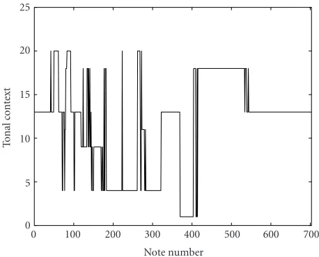
To test the effectiveness of the proposed estimation method in correcting misclassifications in the case of se-quences of key assignments, we apply it to Bach’s Prelude in C Minor from Book II of the Well-Tempered Clavier, which was also studied by Krumhansl [14]. The sequence of key-assignments that is produced by the key-finding algorithm with a window length of 75 is shown inFigure 2. This win-dow length is approximately equal to three measures, a choice that was also made by Krumhansl. The result of applying the proposed estimation method to the sequence of key assign-ments generated by the key-finding algorithm is shown in
Figure 3. A window length of 99 was used. This choice en-ables us to remove any modulations that last less than 50 notes, or approximately two measures. Also, we choosep=1 in (4) in order to directly use the interkey distances and avoid
0 100 200 300 400 500 600 700
Note number
To
n
al
co
n
te
xt
0 5 10 15 20 25
Figure2: The sequence of key assignments for Bach’s Prelude in C Minor from Book II of the Well-Tempered Clavier. The length of the key-finding window is 75.
0 100 200 300 400 500 600 700
c G#
D# c
f
c
Note number
To
n
al
co
n
te
xt
0 5 10 15 20 25
Figure3: The result of applying the proposed estimation method to the sequence of key assignments for Bach’s Prelude in C Minor from Book II of the Well-Tempered Clavier. Upper-case and lower-case letters represent major and minor keys, respectively. The length of the window is 99.
introducing any biases toward small or large distances. Note that while no ordering of the keys was assumed, for purposes of visualizationFigure 3displays the output in the same way asFigure 2.
it usually agrees with their indicated keys of lesser strength. Thus, we can conclude that this approach to localized key finding produces sensible assignments of keys. It also has the advantage that it allows the determination of the key in an ar-bitrary position in the score, that is, the algorithm does not depend on any subdivisions such as measures.1
4. CASE STUDY 2: CORRECTION OF MISCLASSIFICATIONS IN PRIMARY
LOCAL RECOGNITION OF IMAGE FEATURES
In this case study, the proposed estimation method is ap-plied in 2D for correction of misclassifications following clas-sification (primary local recognition) of simulated remotely sensed data. First, in Section 4.1, classification of remotely sensed data is discussed and a method for performing this task is introduced. Then, the requirements for correction of misclassifications are discussed inSection 4.2. In contrast to the case study ofSection 3, in this case there appears to be no theory from which the proximity matrix employed by the es-timation method could be deduced directly, and therefore, in
Section 4.3we employ training-based optimization with ge-netic algorithms as the learning rule for finding the optimal proximity matrix. The accuracy of the obtained classification results is assessed inSection 4.4.
4.1. Classification of remotely sensed data
Remote-sensing systems are widely used for various applica-tions providing valuable data for ecology, hydrology, agricul-ture, and other fields [13,24,25]. These systems commonly include several subsystems that operate in different bands of electromagnetic waves (optical, infrared, microwave). Since the obtained images can cover earth terrains with areas of thousands of square kilometers and the linear resolution of the imaging system is typically of the order of a few me-ters, the obtained images usually contain a very large num-ber (millions) of pixels. Moreover, during many space mis-sions the obtained remotely sensed data have been stored in huge databases, and since some of these missions still con-tinue and other missions are planned in the near future, it is expected that the amount of available data will continue to grow rapidly.
However, the process of obtaining remotely sensed data is only an intermediate step in the course of extracting use-ful information from these data. In this sense, substantial challenges arise in processing the obtained multispectral or multichannel images [24, 25] and ensuring reliable, accu-rate, and appropriately fast extraction of valuable informa-tion [26,27]. It is not reasonable to expect that the required information can be extracted by human experts using visual analysis of the obtained images even if they have at their dis-posal some advanced image processing tools.
One way of addressing this problem is to apply auto-matic procedures of image classification that can be
multi-1Some composers, such as Eric Satie, have chosen to abandon the use of
measures altogether in some of their compositions.
stage or iterative [28]. However, in practice even the most advanced techniques of automatic classification are unable to provide image classification without errors (misclassifi-cations) [26,27]. The main reason is the inherent presence of noise, especially as the characteristics of noise vary widely for different types of images and components of multichan-nel data [29,30]. The correction of misclassifications is thus crucial.
Several versions of possible classification procedures have been developed in [31,32,33,34]. In such procedures, the classification is performed locally and is thus referred to as primary local recognition (PLR). The goal is to classify the central pixel in the sliding window into one of six possible classes:
(i) homogeneous region (H);
(ii) edge between two homogeneous regions having diff er-ent intensity means (E);
(iii) neighborhood of a spike, that is, there is a spike in the sliding window, but not in the central pixel (NS); (iv) spike in the central pixel of the sliding window—this
corresponds to impulsive noise, that is, outliers (S); (v) small-sized or prolonged object in the central pixel—
these are characterized by compactness and connect-edness of pixels as well as by homogeneity of values (O);
(vi) neighborhood of a small-sized object, that is, there is a small-sized or prolonged object in the sliding window, but the central pixel does not belong to it (NO).
This kind of PLR can be very useful for solving many im-portant practical tasks. These include edge detection needed for image segmentation [29] and small-sized object detection required for joint registration of images [35] and automatic target recognition [36]. Another task is the detection and re-moval of outliers. Moreover, after edges and small-sized ob-jects have been detected and localized, it becomes possible to improve image classification in another classification scheme by taking into account neighboring pixels. In other words, PLR results can be useful in further classification of the same scene into, for example, land cover categories such as “for-est,” “water,” and “urban” [30]. Specifically, after detection of edges and, possibly, their thinning, it is intuitively clear that one is in a better position to determine the subset of pixels that correspond to two homogeneous regions forming the considered edge. Similarly, after detection of small-sized objects, the corresponding pixels can be united, allowing for further classification of the considered small-sized objects by applying recognition algorithms that take into account the spatial features of the small-sized object.
membership of the central pixel in the window by using these parameters as features. The details can be found in the aforementioned papers. In this case study, we employ the ap-proach described in [31].
Throughout this case study the image shown inFigure 4
is used as a test image. The image is called “Mosaic” and it is a synthetic 8-bit image of size 256×256. In the image, there is a homogeneous region in the lower part, and in the middle horizontal part there are small-sized objects having different shapes and different numbers of pixels belonging to them. Their contrasts with respect to the background vary as well. In the upper part there are homogeneous regions in-side and between many mosaic-type objects with different shapes, orientations, and contrasts. The idea behind this im-age is to simulate such situations that typically occur in re-motely sensed images.
The primary local recognition stage as well as the used noise model are discussed in detail in [31]. Here it suffices to say that multiplicative Gaussian noise with unit mean and varianceσ2 =0.003 was added to the Mosaic image before PLR.2The result after PLR is shown inFigure 5. Although there are no spikes in the Mosaic image ofFigure 4, there are a lot of pixels for which the PLR algorithm assigns the class NS. This happens due to the fact that classification is done lo-cally. For example, when the sliding window is approaching a small-sized object, the sliding window may contain only one pixel belonging to that object. If all the other 24 pix-els have approximately the same intensity level, the central pixel is classified into NS. Similarly, when the sliding win-dow contains more than one pixel belonging to a small-sized object but the central pixel does not belong to the object, the classification is appropriately NO. These situations occur also with edges (E) between homogeneous regions (H), and thus edges, too, are surrounded by NS as well as NO pixels.
4.2. Requirements for correction of misclassifications
The following requirements are defined for the correction of misclassifications after primary classification:
(R1) E and O pixels should be preserved if they are spatially grouped and they are surrounded by NS and NO pix-els;
(R2) isolated pixels of H, E, and O should be removed; (R3) all pixels with initial classification NS, S, or NO should
be removed.
Since all pixels with initial classification NS, S, or NO should be removed, these classes are considered as supplementary classes, that is, belonging to the multisetBs(seeSection 2). In fact, their primary purpose is to assist in misclassification correction, and as can be seen by looking at requirements (R1) and (R2), the distinction between correctly recognized and misclassified E and O pixels is made primarily on the ba-sis of whether they are surrounded by supplementary classes
2It is shown in [5] that the proposed estimation method can be applied
successfully with higher noise intensities as well.
Figure4: The Mosaic test image.
Figure5: The PLR result of the noisy Mosaic image. The classes H, E, NS, S, O, and NO are shown by gradations of gray from black to white.
Figure6: An example of how correctly classified O pixels are sur-rounded by NS and NO pixels. The classes are H, NS, O, and NO, and are shown by gradations of gray from black to white.
or not. Specifically, correctly classified E and O pixels are sur-rounded by both NS pixels (more distantly) and NO pixels (more closely), whereas this is unlikely to occur for misclas-sified E and O pixels. This property is illustrated inFigure 6. The classes H, E, and O are considered as basic classes, that is, belonging to the multisetBb.
a number of parameters. The above division of classes into basic and supplementary ones leads to the use of (10) (with p=1) as the processing operator. As explained above, here Bb= {H, E, O}andBs= {NS, S, NO}. Further, since a 5×5 window is used in the PLR stage, it is natural to use a 5×5 window here as well. This is because, ideally, a 5×5 neighbor-hood of an E or O pixel contains those supplementary class (NS and NO) pixels that are meant to assist in correction of misclassifications. A larger window would include many H pixels, and correction of misclassifications would be more difficult. A smaller window, in turn, would not include all the information contained in the supplementary classes.
For simplicity, only the central sample is weighted with the spatial weighta=10. The weighting of the central sam-ple increases the probability of the central samsam-ple remaining as the output. This is desired, since it decreases the probabil-ity of a pixel that has been correctly classified in the PLR stage to be misclassified. However, at the same time the probability that a misclassified pixel remains misclassified increases, and therefore, center weighting is a compromise between detail preservation and misclassification correction.
4.3. Training-based optimization
The performance of the proposed method relies on a success-ful choice of the proximity matrix. In this case study, our ap-proach for determining the proximity matrix is to adopt the learning or, as it is known in signal processing, the training-based optimization paradigm. In this framework, it is implic-itly assumed that we can inductively learn from experience and make useful decisions for cases that we have not experi-enced before. Thus, we must employ an empiricist epistemol-ogy, but be able to do so in the presence of uncertainty. This entails making the assumption that different signals and im-ages, despite exhibiting a range of characteristics, will share certain very general properties from which we can make in-ductive inferences. In this case study, all images contain dif-ferent homogeneous regions, small-sized objects, and so on. These characterizations, although very general and unrestric-tive, already inherently impose certain structural regularity that can be exploited in the process of learning. For instance, an image containing homogeneous regions (H) and small-sized objects (O) intrinsically implies that a pixel believed to belong to a small-sized object and yet surrounded entirely by pixels belonging to a homogeneous region is likely to be misclassified.
In general, the size of the search space for the optimiza-tion algorithm, that is, the number of possible proximity ma-trices, is too large for conventional calculus-based or enu-merative optimization algorithms to be useful. In particu-lar, in this case study, there are 18 elements in the proxim-ity matrix and each can take 8 different values (see below), and thus there are 221candidates for the optimal proximity matrix. Moreover, there are typically various local optima in the search space and we therefore have to use a randomized optimization algorithm such as simulated annealing or a ge-netic algorithm (GA). Here, we choose to employ GAs, which are efficient search algorithms based on simulated evolution strategies [2].
Training-based optimization leads to a global combina-torial optimization problem, in which we have a pair (S,f), whereSis a finite or countably infinite set of configurations and f :S→Ris an optimization criterion. The setSis also called the search space or the solution space. In the context of GAs, f is to be maximized and is called the fitness function. The problem is to find a configurations0∈Ssuch that
f(s0)≥ f(s) ∀s∈S. (14) Thus,
s0=arg max
s∈S f(s). (15)
Naturally, minimization problems can be considered simi-larly. The fitness function depends on the particular applica-tion [37].
The goal in the training phase is to find a proximity ma-trix that can be used in correction of misclassifications for a wide range of classified images. The training-based approach also provides a well-defined design methodology. We use a GA that is taken from [2] as the optimization algorithm. We use a fixed population size of 30 individuals. Since the popu-lation size is fixed, two offspring are produced in the recom-bination step. The mutation rate is such that each feature of the offspring can mutate independently with probability 0.03.
The choice of a representative training pair (source image and target image) is crucial. Naturally, since the ultimate goal is to process real remotely sensed images, it would be good to be able to train the method on some representative real radar images. However, for such images it can be difficult to accurately determine the ground truth that is needed for the target image [26]. Therefore, we use the Mosaic image, which is a synthetic image for which the correct classification result can be readily obtained in the noise-free case by using an al-gorithm that is based on simple decision rules. For details of this algorithm, see [6]. The target image is shown inFigure 7
and the source image is shown inFigure 5. The properties of the Mosaic image have already been discussed inSection 4.1. Here, it suffices to say that the image represents a wide range of situations that can occur in practice in correction of mis-classifications and is therefore a suitable training image.
Obviously, the choice of the fitness function is important as well. In our case, the set of all configurationsSis the set of all possible proximity matrices, and the only input parameter of the fitness function is a candidatew ∈Sfor the optimal proximity matrix (the initial candidate is chosen randomly). The real number to be maximized is then f(w). First, the estimation method is applied to the source image using the candidate proximity matrixw. Then, f(w) is the number of pixels in the source image that agree with the corresponding pixels in the target image.
Figure7: The Mosaic target image for training-based optimization. The classes are H (black), E (gray), and O (white).
Figure8: The Mosaic image after the application of the proposed estimation method. The classes are H (black), E (gray), and O (white).
these choices the solution space for the GA is small enough in order for the GA to converge and at the same time it is large enough for the GA to find a satisfactory optimization result. The training phase results in the optimal proximity matrix
Wopt=
H E NS S O NO
0 4 6 7 6 1 7 0 6 5 5 3
− − − − − − − − − − − −
6 7 7 1 1 3
− − − − − −
. (16)
Because a pixel representing one of the supplementary classes S, NS or, NO cannot be an output of (10), the proximities in the third, fourth, and sixth rows do not have an effect on the output of the estimation method, and therefore do not undergo optimization. To emphasize this, those proximities are labeled as “−” in the matrix above.
4.4. Simulations and assessment of accuracy
In the PLR result of the Mosaic image there are 1070 misclas-sified pixels to be corrected (seeFigure 5). Further, there are 19494 pixels representing supplementary classes, which need to be removed in the misclassification correction stage. When the estimation method is applied to the PLR result using the matrix (16), the image shown inFigure 8is obtained. As can be seen, many of the misclassifications have been corrected. To be exact, 733 misclassifications remain, and all the sup-plementary classes have been removed leading to the overall accuracy of 0.989, that is, 98.9 percent of all pixels are clas-sified correctly. Most of the misclassifications are related to edge detection, that is, 668 misclassifications result from an E pixel being committed to the H class or vice versa. How-ever, as there are only 2 discontinuities in edges, this is not a serious problem. The remaining 65 misclassifications are related to recognition of small-sized objects (O).
The number of corrected misclassifications in the Mo-saic image is 498, that is, 46.5 percent of all misclassifications are corrected. It is also worth mentioning that all misclassi-fications, even those that are spatially grouped, are removed from the bottom part of the image in which there is a large homogeneous region. Further, only 6 pixels that are initially recognized correctly in the PLR stage are misclassified by the estimation method. The number of pixels representing sup-plementary classes that are replaced by a wrong class is also relatively low, 155.
An example of edge detection and correction of misclas-sifications in an edge neighborhood is illustrated inFigure 9. A portion of the Mosaic image is presented inFigure 9a. Cor-respondingly,Figure 9bshows the target image for classifica-tion, Figure 9c shows the PLR result, andFigure 9dshows the result after the application of the proposed estimation method. We see that although the edge is recognized reason-ably well in the PLR stage, in addition to many pixels rep-resenting supplementary classes, there are three small-sized object pixels that are clearly misclassifications. Two of these are located in the top right corner of the edge and one in the bottom right corner. Two of these three misclassifications are corrected by estimation method, and at the same time the edge remains continuous. Similarly, an example of small-sized object detection and correction of misclassifications in a small-sized object neighborhood is presented inFigure 10. In this case, the PLR stage results in an image in which two pixels belonging to the small-sized object are misclassified as spike pixels. The result after the application of the estimation method, however, is a perfect classification as can be seen by noting thatFigure 10dis identical toFigure 10b.
(a) (b)
(c) (d)
Figure 9: An example of correction of misclassifications in the neighborhood of an edge. (a) A portion of the original Mosaic im-age, (b) the target image for the portion, (c) the portion after the PLR stage, (d) the portion after the application of the proposed es-timation method. In (b), (c), and (d) the classes H, E, NS, O, and NO are shown by gradations of gray from black to white.
(a) (b)
(c) (d)
Figure 10: An example of correction of misclassifications in the neighborhood of a small-sized object. (a) A portion of the original Mosaic image, (b) the target image for the portion, (c) the portion after the PLR stage, (d) the portion after the application of the pro-posed estimation method. In (b), (c), and (d) the classes H, NS, S, O, and NO are shown by gradations of gray from black to white.
the reference data. The columns represent the reference data whereas the rows indicate the classification whose accuracy is
to be assessed. The error matrix can be given as
E=
n11 n12 · · · n1k n1+ n21 n22 · · · n2k n2+
..
. . .. ... ... ... nk1 nk2 · · · nkk nk+ n+1 n+2 · · · n+k n
, (17)
wherekis the number of classes used by the classifier,ni jgive the number of pixels that are classified into categoryiwhen the correct classification is category j,ni+are the row sums, n+jare the column sums, andnis the sum of all entriesni j. The numbers of correctly classified pixels are given on the main diagonal, that is, wheni= j[26].
An assessment of classification accuracy can be done us-ing a statistical method called Kappa analysis [26]. It is a discrete multivariate technique that is used in accuracy as-sessment for statistically determining if an error matrix is significantly different from another error matrix [38]. The technique was first introduced by Cohen [39] in 1960, and has since then been used in, for example, sociology and psy-chology. It was first published in a remote-sensing journal in 1983 [40], and has since then found popularity in the remote-sensing community. The motivation behind using a statistical-assessment tool such as Kappa analysis is that the overall accuracy, that is, the number of correctly classi-fied pixels divided by the total number of pixels, does not take into account the statistical aspect of the classification result. In particular, in calculating the overall accuracy, the fact that there can be only a small number of pixels repre-senting some class whereas for some other class the number can be very high is not taken into account. In the extreme case, the total number of pixels representing some class can be low enough in comparison to the total number of pix-els in the image under classification for a good overall ac-curacy to be obtained even if most pixels belonging to that class are misclassified. This does not mean, however, that it is not important to be able to obtain a good classification of pixels belonging to some class that has only a few representa-tives.
Kappa analysis puts an approximately equal importance on the correct classification of all classes regardless of the number of pixels representing each class. The result of per-forming a Kappa analysis is the maximum likelihood esti-mate of the Kappa statistic called KHAT and denoted by ˆK. The meaning of the Kappa statistic is that it is a measure of the difference between the actual agreement between the reference data and an automated classifier and the chance agreement between the reference data and a random classi-fier. In other words, the Kappa statistic tells us how statisti-cally significant the improvement in classification accuracy provided by the classifier under assessment is when the clas-sifier is compared against a random clasclas-sifier. In practice, we can calculate the KHAT statistic using the formula
ˆ K=n
k
i=1nii−
k
i=1ni+n+i n2−k
i=1ni+n+i
The KHAT statistic is asymptotically normally distributed even though the data in the error matrix are discrete [26].
Here, the aim of Kappa analysis is to establish that the optimal operator can be used successfully also outside the training data set, that is, that the estimation method with the proximity matrix (16) provides a statistically significant improvement in classification accuracy with images that are significantly different from the Mosaic image. Our set of im-ages includes a total of eight imim-ages. All of these imim-ages are 8-bit images of size 256×256. Like the Mosaic image, they contain edges (E) and small-sized objects (O) of many dif-ferent shapes, sizes and contrasts. In particular, they con-tain shapes and sizes that do not appear in the Mosaic im-age. Moreover, in three of the images there are also pro-longed objects, which are lines that are 1 pixel in thick-ness, and belong to the same class (O) as small-sized ob-jects.
We first apply PLR to all of the eight test images and build the corresponding error matrices. The resulting com-bined error matrix, that is, the sum of the eight error matrices is
Then, we apply the proposed estimation method to all of the eight PLR results and obtain the combined error matrix
E2=
In these error matrices the first row represents the class H, the second row represents the class E, and the third row rep-resents the class O. The grand total of pixels is greater in the second error matrix than in the first one. This is explained by the fact that before the application of the estimation method the image contains 90070 supplementary class pixels that are not accounted for in the first error matrix. The estimation method replaces all the pixels that represent supplementary classes by pixels that represent basic classes, and the grand total increases accordingly.
Examining the error matrices (19) and (20), we imme-diately notice that for each of the three classes the propor-tion of correctly classified pixels is increased. Specifically, the overall accuracy is increased by the application of the esti-mation method from 0.986 to 0.994. We can also look at the ability of the estimation method to correct misclassifica-tions and to avoid introducing new misclassificamisclassifica-tions in the case of our test images. First of all, the number of corrected misclassifications is appropriately high, 3863 (67.4 percent of all misclassifications), which means 483 corrected misclassi-fications per image on the average. On the other hand, the number of misclassifications that are introduced by the esti-mation method is appropriately low, 91, which means less
than 12 new misclassifications per image. The number of supplementary class pixels that are replaced by a wrong class is also quite low, 1056, which means 132 cases per image on the average. These numbers mean that the number of mis-classifications that are present in the test images is reduced from 5733 to 3017 by applying the estimation method. More-over, all of the values are comparable with (and in many cases better than) the corresponding values for the Mosaic image.
Although the number of correctly classified pixels in-creases for all of the three classes, some of the numbers rep-resenting misclassifications, that is, off-diagonal values, in-crease as well. This is mainly due to the fact that some pix-els that represent a supplementary class are misclassified by the estimation method. In spite of these misclassifications, the overall accuracy is increased by the estimation method. However, as explained above, the overall accuracy is not a re-liable measure of the accuracy of a classification. We there-fore calculate the KHAT values for the two error matrices and perform a Kappa analysis. The KHAT values can be cal-culated using (18), and we obtain ˆK1 = 0.9151 and ˆK2 =
0.9545 for the error matrices of before and after the appli-cation of the estimation method, respectively. Thus, like the overall accuracy, the KHAT value is higher after the appli-cation of the estimation method than before its appliappli-cation. In fact, the difference is greater in the KHAT values than in the overall accuracies, which means that the improvement in the classification result that is provided by the estima-tion method is more significant than the overall accuracies suggest.
Finally, hypothesis tests based on confidence intervals around the KHAT value can be made using the approximate large sample variance, which can be computed using the delta method (see, e.g., [26]). The hypothesis test to determine if two independent KHAT values ˆK1and ˆK2, and therefore two error matrices, are significantly different from each other is based on the test statistic
Z= K1ˆ −K2ˆ varK1ˆ + varK2ˆ
, (21)
where var( ˆKi) denotes the approximate large sample vari-ance of ˆKi. The statisticZis standardized and normally dis-tributed. Given the null hypothesisH0 : (K1−K2)=0 and the alternative hypothesisH1: (K1−K2)=0,H0is rejected if Z ≥Zα/2, whereα/2 is the confidence level of the two-tailed Ztest.
5. CONCLUSIONS
An estimation method for correction of misclassifications was presented. The method can be considered as a postclas-sification smoothing operator, because it is intended to be used to correct misclassifications that appear in the output of a classification algorithm based on local context informa-tion. It can be applied to any signal that is comprised of class data regardless of its dimensionality.
Two case studies were presented to illustrate the perfor-mance of the proposed method. These case studies are dif-ferent in many ways. The most notable distinction is that the first takes its example from music and applies the method in 1D, whereas the second applies it in 2D for correcting mis-classifications in simulated remotely sensed images. Further, the approach to finding a suitable proximity matrix is dif-ferent in the case studies. In the first, the proximity matrix is derived directly from music perception studies, whereas in the second, training-based optimization using genetic al-gorithms is employed. The applications of the case stud-ies also require significantly different numbers of classes — 24 and 6, respectively. The sizes of the sliding window are also significantly different being 99 and 25 samples, respec-tively. Nonetheless, the proposed method is found to pro-vide a good misclassification correction result in both case studies.
ACKNOWLEDGMENTS
The support of the Academy of Finland is gratefully ac-knowledged. V. V. Lukin is supported by the Project Grant 1659 of the Scientific Technology Center of Ukraine. A. N. Dolia is supported by Engineering and Physical Sci-ence Research Council Grant GR/R61215, UK, and by Data and Information Fusion, Defence Technology Center Grant, UK.
REFERENCES
[1] R. Dubes and A. K. Jain, “Random field models in image anal-ysis,”J. Appl. Stat., vol. 16, no. 2, pp. 131–164, 1989. [2] D. Goldberg, Genetic Algorithms in Search, Optimization,
and Machine Learning, Addison-Wesley, Reading, Mass, USA, 1989.
[3] A. H. S. Solberg, T. Taxt, and A. K. Jain, “A Markov random field model for classification of multisource satellite imagery,” IEEE Transactions on Geoscience and Remote Sensing, vol. 34, no. 1, pp. 100–113, 1996.
[4] V. V. Lukin, I. Shmulevich, O. P. Yli-Harja, and A. N. Do-lia, “Correction of misclassifications in primary local image recognition using a nonlinear graph-based estimation tech-nique,” inImage and Signal Processing for Remote Sensing VI, S. Serpico, Ed., vol. 4170 ofProceedings of SPIE, pp. 251–259, Barcelona, Spain, January 2001.
[5] A. Niemist¨o, V. V. Lukin, A. N. Dolia, O. P. Yli-Harja, and I. Shmulevich, “Misclassification correction in primary lo-cal recognition of component images of multichannel remote sensing data,” inImage and Signal Processing for Remote Sens-ing VII, S. Serpico, Ed., vol. 4541 ofProceedings of SPIE, pp. 134–145, Toulouse, France, September 2001.
[6] A. Niemist¨o, V. V. Lukin, I. Shmulevich, O. P. Yli-Harja, and A. N. Dolia, “A training-based optimization framework for misclassification correction,” inProc. 12th Scandinavian Con-ference on Image Analysis (SCIA ’01), pp. 691–698, Bergen, Norway, June 2001.
[7] O. P. Yli-Harja and I. Shmulevich, “Correcting misclassifi-cations in hyperspectral image data using a nonlinear graph-based estimation technique,” inProc. International Sympo-sium on Nonlinear Theory and Its Applications (NOLTA ’99), pp. 259–262, Waikoloa, Hawaii, USA, November 1999. [8] O. P. Yli-Harja, I. Shmulevich, and K. Lemstr¨om,
“Graph-based smoothing of class data with applications in musical key finding,” inProc. IEEE-EURASIP Workshop on Nonlinear Sig-nal and Image Processing, pp. 311–315, Antalya, Turkey, June 1999.
[9] D. Johnson and W. Wang, “Symbolic signal processing,” inProc. IEEE Int. Conf. Acoustics, Speech, Signal Processing (ICASSP ’99), pp. 1361–1364, Phoenix, Ariz, USA, March 1999.
[10] F. R. McMorris, H. M. Mulder, and R. C. Powers, “The median function on median graphs and semilattices,”Discrete Applied Mathematics, vol. 101, no. 1-3, pp. 221–230, 2000.
[11] F. R. McMorris and R. C. Powers, “The median procedure in a formal theory of consensus,”SIAM J. Discrete Math., vol. 8, no. 4, pp. 507–516, 1995.
[12] J. T. Astola and P. Kuosmanen, Fundamentals of Nonlinear Digital Filtering, CRC Press, Boca Raton, Fla, USA, 1997. [13] T. Lillesand and R. Kiefer,Remote Sensing and Image
Interpre-tation, John Wiley & Sons, New York, NY, USA, 1994. [14] C. Krumhansl,Cognitive Foundations of Musical Pitch, Oxford
University Press, New York, NY, USA, 1990.
[15] S. Holtzman, “A program for key determination,” Interface, vol. 6, no. 1, pp. 29–56, 1977.
[16] H. Longuet-Higgins and M. Steedman, “On interpreting Bach,” inMachine Intelligence, B. Meltzer and D. Michie, Eds., vol. 6, pp. 221–241, University of Edinburgh Press, Ed-inburgh, Scotland, 1971.
[17] P. Vos and E. van Geenen, “A parallel-processing key-finding model,”Music Perception, vol. 14, no. 2, pp. 185–224, 1996. [18] E. J. Coyle and I. Shmulevich, “A system for machine
recog-nition of music patterns,” inProc. IEEE Int. Conf. Acoustics, Speech, Signal Processing (ICASSP ’98), pp. 3597–3600, Seat-tle, Wash, USA, May 1998.
[19] I. Shmulevich and O. P. Yli-Harja, “Localized key-finding: Al-gorithms and applications,” Music Perception, vol. 17, no. 4, pp. 531–544, 2000.
[20] I. Shmulevich, O. Yli-Harja, E. Coyle, D.-J. Povel, and K. Lem-str¨om, “Perceptual issues in music pattern recognition: Com-plexity of rhythm and key finding,” Computers and the Hu-manities, vol. 35, no. 1, pp. 23–35, 2001.
[21] I. Shmulevich and E. J. Coyle, “The use of recursive me-dian filters for establishing the tonal context in music,” in Proc. IEEE Workshop on Nonlinear Signal and Image Process-ing, Mackinac Island, Mich, USA, 1997.
[22] C. Krumhansl and E. Kessler, “Tracing the dynamic changes in perceived tonal organization in a spatial representation of musical keys,” Psychological Review, vol. 89, no. 4, pp. 334– 368, 1982.
[23] J. Kruskal and M. Wish,Multidimensional Scaling, Sage Pub-lications, Beverly Hills, Calif, USA, 1978.
[24] W. Keydel, “SAR technique and technology, its present state of the art with respect to user requirements,” inProc. 1st Euro-pean Conf. Synthetic Aperture Radar, pp. 19–24, K¨onigswinter, Germany, March 1996.
Radar (SIR-C/X-SAR),” IEEE Transactions on Geoscience and Remote Sensing, vol. 33, no. 4, pp. 817–828, 1995.
[26] R. Congalton and K. Green,Assessing the Accuracy of Remotely Sensed Data: Principles and Practices, CRC Press, Boca Raton, Fla, USA, 1999.
[27] D. Landgrebe, “Information extraction principles and meth-ods for multispectral and hyperspectral image data,” in In-formation Processing for Remote Sensing, C. H. Chen, Ed., pp. 3–38, World Scientific Publishing, River Edge, NJ, USA, 1999. [28] B. Solaiman, L. Pierce, and F. Ulaby, “Multisensor data fusion using fuzzy concepts: application to land-cover classification using ERS-1/JERS-1 SAR composites,” IEEE Transactions on Geoscience and Remote Sensing, vol. 37, no. 3, pp. 1316–1326, 1999.
[29] J. Richards and X. Jia, Remote Sensing Digital Image Analy-sis: An Introduction, Springer-Verlag, Berlin, Germany, 1999, edited by W. Gessner and D. Ricken.
[30] V. V. Lukin, J. T. Astola, V. Melnik, et al., “Data fusion and processing for airborne multichannel system of radar remote sensing: Methodology, stages, and algorithms,” in Sensor Fusion: Architectures, Algorithms, and Applications IV, B. Dasarathy, Ed., vol. 4051 ofProceedings of SPIE, pp. 215– 226, Orlando, Fla, USA, April 2000.
[31] A. N. Dolia, A. Burian, V. V. Lukin, C. Rusu, A. A. Kurekin, and A. A. Zelensky, “Neural network application for primary local recognition and nonlinear adaptive filtering of images,” inProc. 6th IEEE Conference on Electronics, Circuits and Sys-tems, pp. 847–850, Pafos, Cyprus, September 1999.
[32] A. N. Dolia, V. V. Lukin, A. Kurekin, A. Zelensky, N. Pono-marenko, and A. Sokolov, “Modified image local recognition system for locally adaptive filtering,” inProc. 6th Int. Symp. Automatic Control and Computer Science, pp. 84–89, Iasi, Ro-mania, November 1998.
[33] A. N. Dolia, V. V. Lukin, A. Zelensky, J. T. Astola, and C. Anag-nostopoulos, “Neural networks for local recognition of im-ages with mixed noise,” inApplications of Artificial Neural Net-works in Image Processing VI, N. Nasrabadi and A. Katsaggelos, Eds., vol. 4305 ofProceedings of SPIE, pp. 108–118, San Jose, Calif, USA, January 2001.
[34] V. V. Lukin, N. Ponomarenko, J. T. Astola, and K. Saarinen, “Algorithms of image nonlinear adaptive filtering using frag-ment recognition by expert system,” inNonlinear Image Pro-cessing VII, E. R. Dougherty, J. T. Astola, and H. G. Long-botham, Eds., vol. 2662 ofProceedings of SPIE, pp. 179–190, San Jose, Calif, USA, March 1996.
[35] G. P. Kulemin, V. V. Lukin, A. A. Zelensky, A. A. Kurekin, and E. T. Engman, “Soil-erosion-state interpretation using pre- and postprocessing of multichannel radar images,” in Remote Sensing for Agriculture, Ecosystems, and Hydrology II, E. T. Engman, Ed., vol. 3499 ofProceeding of SPIE, pp. 134– 144, Barcelona, Spain, December 1998.
[36] F. Sadjadi, H. Nasr, H. Amehdi, and M. Bazakos, “Knowledge-and model-based automatic target recognition algorithm adaptation,” Optical Engineering, vol. 30, no. 2, pp. 183–188, 1991.
[37] P. Koivisto, H. Huttunen, and P. Kuosmanen, “Training-based optimization of soft morphological filters,” Journal of Elec-tronic Imaging, vol. 5, no. 3, pp. 300–322, 1996.
[38] Y. Bishop, S. Fienberg, and P. Holland, Discrete Multivariate Analysis: Theory and Practice, MIT Press, Cambridge, Mass, USA, 1980.
[39] J. Cohen, “A coefficient of agreement for nominal scales,” Educ. Psychol. Meas., vol. 20, no. 1, pp. 37–46, 1960.
[40] R. G. Congalton and R. A. Mead, “A quantitative method to test for consistency and correctness in photo-interpretation,”
Photogrammetric Engineering and Remote Sensing, vol. 49, no. 1, pp. 69–74, 1983.
Antti Niemist¨owas born in Tampere, Fin-land in 1977. He received the M.S. degree with honours in computer science in 2002 from Tampere University of Technology, Tampere, Finland. From 2002 to present he has been a Ph.D. student at the same univer-sity. In 2003 and 2004 he was a Research In-tern at The University of Texas M. D. Ander-son Cancer Center, Houston, Texas, USA. Currently he is a Researcher with the
Insti-tute of Signal Processing of Tampere University of Technology. His research interests include nonlinear signal and image processing, image analysis, and bioinformatics.
Ilya Shmulevich received the Ph.D. de-gree in electrical and computer engineer-ing from Purdue University, West Lafayette, Indiana in 1997. From 1997 to 1998, he was a postdoctoral researcher at the Ni-jmegen Institute for Cognition and Infor-mation, University of Nijmegen, Nijmegen, the Netherlands, and National Research In-stitute for Mathematics and Computer Sci-ence, University of Amsterdam,
Amster-dam, the Netherlands, where he studied computational models of music perception and recognition. From 1998 to 2000, he was a se-nior researcher at the Tampere International Center for Signal Pro-cessing, Signal Processing Laboratory, Tampere University of Tech-nology, Tampere, Finland. Presently, he is an Assistant Professor with the Cancer Genomics Laboratory, The University of Texas M. D. Anderson Cancer Center, Houston. His research interests in-clude computational genomics, nonlinear signal and image pro-cessing, computational learning theory, and music recognition and perception.
Vladimir V. Lukinwas born in 1960 in Be-larus (former Soviet Union). He graduated in 1983 from the Faculty of Radioelectronic Systems, Kharkov Aviation Institute (now National Aerospace University), Kharkov, Ukraine, and received the Diploma degree with honours in radioengineering. Since then, he has been with the Department of Transmitters, Receivers, and Signal Process-ing of the same faculty. He received
Alexander N. Doliareceived the M.S. de-gree with distinction in computer science from the Kharkov Aviation Institute (now National Aerospace University), Kharkov, Ukraine in 1994 and the Ph.D. degree in radio engineering from the National Aerospace University, Kharkov, Ukraine in 2001. From 1988 to 1989 he was an operator of optical tracking systems with the tracking and monitoring stations, USSR Air Forces,
Priozersk, Kazakhstan. Since 1994 he has been associated with the Department of Transmitters, Receivers, and Signal Processing of the Faculty of Radio-Engineering Systems, National Aerospace University, Kharkov, Ukraine as a research fellow. From 2002 to 2003, he was a postdoctoral research fellow with the Department of Psychology, University of Glasgow, Scotland, where he stud-ied computational models of visual cortex and human motion with emotions. Currently, he is a postdoctoral research fellow with the Electronics and Computer Science Department, University of Southampton, England. His research interests include target detec-tion/classification and tracking, statistical machine learning, mul-tisensor active management, data mining, bioinformatics, and vi-sion.
Olli Yli-Harjareceived the Doctor of Tech-nology degree in computer science and ap-plied mathematics from Lappeenranta Uni-versity of Technology, Finland, in 1989. During the years 1988–1998 he was a Re-search Scientist and a Lecturer in computer science, at the Technical Research Centre of Finland, Helsinki University of Technology, and University of Helsinki. In 1998 he was a research fellow at East Anglia University,