R E S E A R C H
Open Access
Modeling and analysis of random dense
CSMA networks
Yuhong Sun
1*, Ruinian Li
2, Honglu Jiang
1, Jianchao Zheng
1and Lina Ni
3,4Abstract
The MAC (medium access control) of CSMA (carrier sense multiple access) is widely used in distributed wireless networks with random node locations. In CSMA MAC, two nodes that are within the range of one another cannot transmit packets simultaneously. Modeling the concurrently transmitting nodes is crucial for the performance analysis of the CSMA networks. In this paper, we study the density of concurrently transmitting nodes and propose another modification of classical hard core point process to accurately estimate the density of concurrently transmitting nodes, in the absence and in the presence of fading conditions. The MMHCP model we propose outperforms the popular Matérn type II model and the existing modified hard core point (MHCP) process model by avoiding the underestimation and alleviating the overestimation issues, respectively. We conduct extensive
numerical analysis and simulations to evaluate the accuracy of our MMHCP model. Furthermore, we study the impact of the density of initial Poisson Point Process (PPP) and fading factor on the mean probability of successful reception and on the transmission capacity of networks from numerical analysis and simulations.
Keywords:CSMA, Stochastic geometry, Hard core point process, Density, SIR
1 Introduction
In distributed wireless networks with random node loca-tions, such as ad-hoc networks or sensor networks, cogni-tive femtocell networks, a decentralized medium access control (MAC) protocol is required to control the access of the network nodes to the shared wireless spectrum in order to limit the mutual interference. With the low cost of the wireless network technologies, the nodes deployed in wireless networks are becoming denser and denser. For example, the last few years have witnessed the prolifera-tion of WiFi Access Points (APs) in many urban areas, and it is very common that several APs are in the commu-nication range of each other. In other examples such as in the hot-spot networks [1] or cyber-physical systems [2], with a growing number of sensors being deployed, more and more data will be transmitted over wireless links.
For this type of networks, carrier-sense multiple access (CSMA) protocols are very popular to avoid collisions and improve the network performance. CSMA distin-guishes itself with its distributed nature in coordinating
the spectrum access. Under CSMA/CA (Carrier sense multiple access with collision avoidance), a transmitter continuously senses the channel state prior to transmit-ting. If the channel state is idle, the transmitter starts to transmit packets. Otherwise, it waits for a while before it starts sensing the status. By this way, the network can reduce the interference to achieve a higher probability of successful transmissions and higher network capacity.
In the studies of CSMA protocol, there are several problems that must be considered, such as hidden ter-minals [3], starvation, or fairness in heavily loaded
net-works [4, 5]. Many work focus on designing a better
MAC protocol to overcome some flaws or improve some performance, for example [4–7]. In light of modeling the CSMA networks, traditional method typically rely on Markovian approaches. However, Markovian models fail to represent physical layer effect, such as the impact of fading and cumulative interference. In this paper of our work, we focus on modeling the concurrently transmit-ting nodes under CSMA protocol and analyzing interfer-ence via stochastic geometry. The modeling and analysis on the concurrently transmitting nodes can be used in many distributed wireless networks with CSMA protocol * Correspondence:sun_yuh@163.com
1School of Information Science and Engineering, Qufu Normal University, Yantai Road 80, Rizhao 276826, People’s Republic of China
Full list of author information is available at the end of the article
to evaluate the interference and the relevant network performance.
The introduction of stochastic geometry to analyze the network performance from a statistical perspective has been more than three decades [8]. In stochastic geom-etry, the Poisson Point Process (PPP) is widely used in modeling the topology of networks, such as cellular net-works in [8–10] and ad-hoc networks in [11], for its tractability in analyzing the network performance. How-ever, the PPP is accurate for very sparse networks as the distribution of the atoms of a PPP is independent, which is not always the exact case in wireless networks. For ex-ample, in heterogeneous cellular networks, the locations of base stations are modeled by Poisson Cluster Process (PCP) in [12] or by Ginibre Point Process (GPP) in [13], in order to reflect the dependence of the locations of the base stations. Similarly, due to the exclusion of CSMA nodes, the hard core point process (HCPP), instead of PPP, is usually applied to model the simultaneously transmitting nodes.
Among the hard core point processes, Matérn type II model is most widely used in modeling CSMA networks. Although Matérn type I model can get a legitimate HCPP, it is proved that this model only accounts for retaining the isolated points (i.e., points which are at least fixed distance away from every other point in the process). While Matérn type II model captures the con-tention among the initial points to be retained in the HCPP. Furthermore, the author in [14] proved that Matérn type II model can be approximated by a non-homogeneous PPP. Many work such as [15–19] modeled the CSMA networks by Matérn type II model.
The Matérn type II model can be obtained by thinning a PPP as follows. Let Φ= {xi}i∈(1,n) be a homogeneous PPP. Each point xi is marked by a random variable mi that is uniformly distributed between [0,1]. The marks are independent and identically distributed, or i.i.d, and independent of the positions ofxi. If the ball that centers at xi with radius h does not consist of any points with mark less than mi, the point xi is retained in the hard core point process. The points that are not retained will be deleted from the PPP in the end. Since whether a point is retained or not is determined by points around it, the thinning process is not independent.
As stated in many literatures such as [15, 17, 20, 21], Matérn type II model tends to lead an underestimation of the transmitting nodes’ density. As shown in Fig. 1, node x1 is not retained as it detects its neighbor x2; moreover, node x2is not retained either, as it detects its neighbor x3, i.e., m1>m2>m3, where mi is the mark of
xi. As a result, neither x1nor x2 can be retained in the thinning scheme. However, if x3 is not the neighbor of
x1, and ifx3does not detect any on-going transmissions of its neighbors, a more reasonable MAC will allow x1 andx3to transmit simultaneously.
That is mainly because the freezing property of the backoff timer in the CSMA protocol is not captured to calculate the density of the simultaneously active transmit-ters in the Matérn type II model. In a CSMA network, a transmitter still can access the channel if it does not have the lowest backoff time in its contention domain given that all of the transmitters with lower backoff time have frozen their timers. A model named Matérn type III is de-fined as completely capturing the freezing property, while
it involves a chain of correlations among the initial points (potential transmitters). The chain terminates when it reaches a point (transmitter) which is definitely retained or not. Therefore, Matérn did not discuss such a model more and regarded it“rather formidable”[20].
In [20, 21], the authors investigated the problem of underestimation of the Matérn type II model and pro-posed a second-order density estimation model, named MHCP, that partially takes the backoff timer freezing property into consideration and reduces the underesti-mation of density due to Matérn type II modeling. This model is called to“go one step in the correlation chain” and gives corresponding expression on the density, out-age probability, and transmission capacity in [20]. How-ever, their model tends to overestimate the transmitting node density in dense CSMA networks, especially in fad-ing environment.
In this paper, we propose a new idea on the correlation chain and restrain that any nodes in the network have a same retaining probability in statistical meaning, or take the mean probability of retaining a node in the network to make the density analysis tractable, which is proved that our model can also avoid the transmitting density underestimation of Matérn type II model and alleviate the overestimation of MHCP in [20, 21]. The constraints make the model still applicable in the distributed wireless network, such as in bipolar model of MANET [17], wireless sensor networks [22–24], or one tier of multi-tier heterogeneous networks [10] where the nodes in the same tier have same properties.
The multi-fold contributions can be summarized as follows.
(i). We analyze the Matérn type II model and the MHCP model to demonstrate that the Matérn type II model underestimates while the MHCP tends to overestimate the density in dense networks and fading environment.
(ii).We propose another modification of Matérn type II model based on MHCP to estimate the retaining probability for a node in the initial PPP and then the transmitting density for the CSMA networks. (iii).We get the density expression for the simultaneously
transmitting nodes in dense CSMA networks given that nodes being retained by a same probability in statistical meaning. This is another partial solution for the“correlation chain”of Matérn type III model, other than [20,21]. Furthermore, we generalize the model in Rayleigh fading.
(iv).We analyze the mean probability of successful reception and transmission capacity in CSMA networks based on the proposed model and reveal the mean probability of successful reception being almost immune to the fading and the initial intensity, while the transmission capacity of the
network tends to be closer to our proposed model with the increased fading factor.
The rest of our paper is organized as follows. Section 2reviews the related work. In Section3, we give the net-work model, assumptions, and the methodology of ana-lyzing models. Section 4 gives the retaining probability and network transmitting density of the proposed model in the deterministic fading, and Section5generalizes the model under Rayleigh fading. The network performance including the successful reception probability and trans-mission capacity is given in Section6. Section 7 demon-strates the numerical and simulation results, and the last section concludes this paper. A list of the key mathemat-ical notations used in this paper is given in Table1.
2 Related work
There are many work on the interference management and performance analysis using stochastic geometry, mainly for the PPP model, such as [9–11]. For the added complexity, there are not so many results on the HCPP modeling and analysis. In this section, we review the work closely related to the HCPP and our work.
The author in [14] proved that there is no known ex-pression for the probability generating functional for the HCPP, and it is extremely difficult to find the exact dis-tribution of the aggregate interference. The author com-pared the Matérn type I and Matérn type II model and proved that the Matérn type II model can be safely ap-proximated by an inhomogeneous PPP model for interference-based performance analysis.
result. However, the contention resolution process pre-sented by above literatures all follows the Matérn type II model. Some of them mentioned the underestimation of density for the active nodes [15–17], but no essential im-provement of the underestimation is mentioned.
Simple Sequential Inhabitation (SSI) is an alternative to model the dense CSMA networks. It is derived from the packing and space-filling problems. The authors in [26,27] used SSI to model the spatial distribution of potential inter-ference sources. However, analyzing the model turned out to be very challenging as SSI gives the point density only
when the underlying PPP density tends to be infinity and cannot derive an analytical expression.
To overcome the underestimation for density of Matérn type II model, the authors in [20,21] proposed a modified hard core point (MHCP) process. In MHCP, a nodexihas the privilege to transmit in a time slot for the following two reasons. First, nodexihas the lowest mark in its con-tention domain, which is as same as that in the Matérn type II model. Second, nodexihas the second lowest mark in its contention domain, and nodexjhas the lowest mark while xj is not the node with the lowest mark in conten-tion domain of itself. Such a scheme is called“go one step in correlation chain”[20], which actually can avoid omit-ting some nodes. With channel conditions deteriorate, es-pecially in a network with dense nodes, the MHCP model tends to overestimate the transmitting density of the net-work [20], as shown in Fig. 2. The nodes x3and x4are retained for they have the lowest mark in their contention domains, and nodesx1,x2,x5, andx6are retained for they have the second lowest mark in their contention domains, while the corresponding nodes with the lowest mark (x2,
x5,x6,x7) are not the one with the lowest mark in the con-tention domain of themselves. But a reasonable scheme would retainx3,x4,x1, andx5orx3,x4,x2, andx6. That is because when they considered the nodes with second low-est mark, the nodes with the lowlow-est mark may be retained for the same reason, resulting in two nodes being retained at the same time in one domain.
In this paper, we consider the problem of underestima-tion and overestimaunderestima-tion from a new perspective. That is, in the initial PPP, a nodexiis retained under the following conditions: (1)xihas the lowest mark in its contention do-main; (2)xihas the second lowest mark in its contention domain; and meanwhile, node xj has the lowest mark in the contention domain of xi, and xj is not retained. We name our proposed model as modification of MHCP (MMHCP). The idea seems like the correlation chain in Matérn type III at first sight. Then, we analyze it by adding the constraint that nodes in a network have a same retain-ing probability in statistical meanretain-ing.
3 Network model, method, and notations 3.1 Network model
We use a marked Poisson point processΦ~ ¼ fðxi;miÞg to indicate the potential transmitters contending to access the spectrum, where {xi} is a homogeneous PPP over the plane with density λp, denoting the locations of the potential transmitters. The {mi} denotes the backoff time of a node, that is uniformly distributed in the range [0,1], similar as in [15, 17, 20, 21]. Although the backoff time is usually not uniformly distributed between [0,1] in the actual protocol (binary exponential backoff, for example), it is proved in [28] that assuming a uniform distribution for the time
Table 1List of key abbreviations
Notation Description ~
Φ Potential transmitters (the initial PPP) contending to access the spectrum
~
Φt Concurrently transmitting nodes under CSMA protocol
xi Location of a node and the node itself
Pt Transmitting power of each transmitter
gij Fading channel gain of the link between nodexi and nodexj
Fij Virtual power emitted from nodexito nodexj
P0 Power threshold for a node to sense another transmitting node
μ Rayleigh fading factor
β Path loss exponent
re Distance threshold for a node sensing another transmitting node
N(xi) Neighborhood of nodexi
Ci Contention domain of nodexi, and the set of nodes coexisting withxiin the domain
T SINR threshold for a receiver can successfully decode
N Average number of neighbor nodes for nodexi without fading
M Average number of nodes in the shadow (Fig.4) without fading
~
N Average number of neighbor nodes for nodexiwith fading
~
M Average number of nodes that cannot be sensed by nodexiwhile can be sensed byxjwith fading
~
P Average number of nodes that can be sensed both byxiandxjsimultaneously
Pretain[i] Probability of a nodexibeing retained
P1[i],Pmin[i] Probability of a nodexihaving the lowest mark in its neighborhood set
P2[i] Probability of a nodexihaving the second lowest mark in its neighborhood set
P2_retain[i] Probability of a nodexiwith the second lowest mark in its neighborhood set being retained
Pi½j Probability of nodexjhaving the lowest mark in Ci, andxjnot being retained
e_ps Mean probability for a node successful reception
marks does not affect the generality of the model. The power emitted from xi (provided it is authorized by the
MAC mechanism) towards xj is denoted by F
j i ¼Pt:g
j i,
where Pt is the transmitting power and gij is the fading channel gain of the link between nodexiand nodexj.
Assume the transmitting power being same, the value of
Fij is same for all nodes if we consider the fixed fading or no fading. In this paper, we also consider the fading envir-onment, named Rayleigh fading, of which the fading chan-nel gain is subject to an exponential distribution with parameterμ, μ> 0. Generally, due to the characteristic of Rayleigh fading,gijis independent for different links.
The neighborhood of a node is defined asNðxiÞ ¼ fjj ð xi;miÞ∈Φ~ : Fij=lðjxi−xjjÞ≥P0g, where P0>0 is the sensing
threshold of the network andl(.) is the path loss function, which is usually taken as l(r) =rβ, β> 2, where r is the distance between a transmitter and its receiver. For simplicity, we denote the contention domain of nodexias
Ci. It is easy to see that if we consider the fixed fading, the same transmitting power and the same sensing threshold for each node, the contention domain is actually a disk with a certain radius re. On the other hand, in a fading environment, the contention domain is not a regular shape due to the random channel gain, as stated in [20].
We assume that the receivers are randomly distributed over the plane with another PPP, which is irrelevant to the transmitters. The number of receivers is enough to
guarantee each active transmitter has one receiver at least in a time slot. A receiver associates with the trans-mitter that provides the strongest average received power conditioned that the receiver can be sensed by the transmitter. This means that each active transmitter associates with the nearest receiver. Once an association is fixed, other active transmitters are treated as interfer-ence. Figure3illustrates an example of the model, where the potential transmitters are denoted by red stars, the transmitting nodes and the receivers are denoted by blue circles and blue triangles respectively. The intended links are denoted by solid arrows, and some interference links of a receiver are denoted by dot lines.
As previous work, in recent research of wireless network such as [29–31], the signal to interference plus noise ratio (SINR) is taken as a metric of successful transmission for an intended link. In dense networks of this paper, the influ-ence of noise can be neglected, namely, interferinflu-ence-limited network. The probability of successful reception can be expressed as ps=Pro[SIR>T], where SIR is the ratio of intended signal to the aggregate interference, andT is the threshold that the receiving node can successfully decode.
3.2 Method
In this paper, we firstly focus on the model of the trans-mission without fading. Under such a case, there is only one source of randomness due to the spatial distribution of the nodes. It is easy to analyze the retaining probability
Fig. 2Density overestimation in MHCP model. Nodes around red circle would be retained. The nodesx3andx4are retained for they have the
lowest mark in their contention domain, and nodesx1,x2, andx5, x6are retained for they have the second lowest mark in their contention
domains, while the corresponding nodes with the lowest mark (x2, x5, x6, x7) are not the one with the lowest mark in their contention domains. A
of a node from the potential transmitters, since the dis-tance threshold for a node sensing other transmitters is fixed, asre= (Pt. g/P0)1/β(in Matérn type hard core point process, the exclusion radius is given as a fixed value). The contention domain, or the neighborhood of a node, can be regarded as a disk with fixed radius as re. Meanwhile,
the area of the domain sensed by two nodes
simultaneously, and the area of the domain sensed by node xiand not sensed by another node xj (whenxi has the second lowest mark, andxjhas the lowest mark in the contention domain of xi) can be derived based on the probability and statistics information. We can calculate the average number of nodes in above domains, respectively. The transmitting density and the aggregate interference can be derived accordingly, as [21].
However, when the model is applied to fading scenarios, another randomness due to the random channel gains is added in the network model. In such a case, the receiving power is not determined, even both the transmitting power and the link distance are fixed. Accordingly, the distance threshold for a node sensing another node is random. Nei-ther the contention domain of one node, nor the domain sensed by two nodes simultaneously, is not a region with a fixed area or fixed shape. Fortunately, the randomness stems from the fading, so we can catch it from the fading factors. Knowing the fading factor, the average number of nodes sensed by a nodexi, or the average number of nodes sensed by two nodesxi,xjsimultaneously (whenxihas the second lowest mark, and xjhas the lowest mark in the contention domain of xi) can be expressed with the instantaneous
distance thresholdre. Therefore, the result on the retaining probability, transmitting density, and related metric in the model without fading can be extended to the model with fading condition. The difference from the model without fad-ing is that the distance thresholdreis random following with the fading factor at different directions, and at any time slot. In [20], the authors utilized a circular bounding box around the irregular contention domain to make the analysis tract-able and derived a lower bound to the number of transmit-ters in the neighborhood of a node. Different from the bounding approach, our method considers the average num-ber of the transmitters in the contention domain of a node following with the random variable(reandμ) and derive the mean retaining probability and the transmitting density, which is consistent with the constraint added in our model. Such analysis is applicable to the overall performance of the network.
3.3 Notations
For the sake of argument, we specify some of the key mathematical notations listed in Table1. Node xiis ab-breviated asi, andi,j, andkare used to denote different nodes. We use Ci to denote both the nodes set in the contention domain of nodeiand the contention domain itself. The following probabilities are essential to deter-mine whether a node is privileged to transmit.
Probability of a node i being retained is denoted by
Pretain[i] = Pro[iis retained].
Probability of a nodeihaving the lowest mark inCiis denoted byP1[i] =Pmin[i].
Probability of a nodeihaving the second lowest mark inCiis denoted byP2[i].
Probability of a nodeiwith the second lowest mark in
Cibeing retained is denoted byP2_retain[i].
Probability of a node j having the lowest mark in Ci and not being retained, conditioned on that node i has the second lowest mark, is denoted byPi½j.
Suppose there are n nodes coexisting with node xi in its contention domain. Due to the uniform distribution
of the marks among the n + 1 points in Ci, and the
marks are irrelevant to the points, the probability thatxi has a certain mark (among then+ 1 marks) equals to 1/ (n+ 1). At the same time, since we adopt a homoge-neous PPP, the average number of points in Ci is λpSCi, whereSCiis the area ofCi. With the fixed fading,SCican be the area of a disc with radiusre. Hence, the probabil-ityP1[i] andP2[i] can be derived as follows.
the above probability can be written as1−e−N
N .
Suppose xi has the second lowest mark in Ci, and xj has the lowest mark, while there is at least one node xk in Cj with a lower mark than mj. It is equivlant to say that there is at least one node with lower mark than mj inCj−Ci(shadow of Fig. 4). The probability is Pro½∃k∈ð
average number of the Cj−Ci. The derivations can be found in [21]. We use PCj−Ci½k to indicate this similar
scenario in the rest of the paper. Therefore, the probabil-ity of a node being retained on that having the second lowest mark is we consider the fixed fading or no fading conditions, the
deduction of M can be found in [21]: M¼λp
The above expression can be manipulated in a closed form. We can further plug it into (2) to get the probability of a node with the second lowest mark being retained in MHCP. The whole retaining probability for a node is
PMHCP=Pmin+P2_retain.
4 Base analysis of MMHCP
Combining the analysis of Matérn type II model and the MHCP model, we propose the MMHCP model to estimate the retaining probability of initial deployed nodes. In this section, we firstly focus on the condition that fading is uni-form, or fixed fading. In MMHCP model, we consider the simultaneously transmitting nodes (retained nodes) under CSMA protocol include those nodes with the lowest mark and the nodes that have the second lowest mark in the do-main of itself while the node with the lowest mark has not been retained. It can be formally expressed as follows:
~
Φt¼ fxi:∀xj∈NðxiÞ;xi≠xj;mi<mjg∪fxi:∃xj∈NðxiÞ;mi>mj;∀
-xk∈NðxiÞnfxi;xjg;mk>mi;xjis not retainedg. The
prob-ability of a node been granted to transmit is
Pretain½i ¼P1½i þP2½i Pi½j, where Pi½jis the
probabil-ity of node jhaving the lowest mark inCi and not being retained.
The difference between MMHCP and MHCP is the retaining probability of the node with the second lowest mark in its contention domain. In MHCP, if a node xi has the second lowest mark in Ci, it is retained only if the node with the lowest markxjis not the one with the lowest mark in Cj. In MMHCP, a node xi with the sec-ond lowest mark in Ci is retained because nodexj with the lowest mark is not retained. Even if nodejdoes not have the lowest mark in Cj, it may be retained for the same reason as nodei. When this occurs, nodeishould not be retained. However, in MHCP model, node i will be retained in the same case, which leads to the overesti-mation of the number of retained nodes.
For Pi½j, it can be interpreted as the condition that node i has the second lowest mark in Ci, while node j
has the lowest mark in Ci and is not retained. In other words, node i has the second lowest mark in Ci, and node j is not retained only because there is at least a node k in Cj−Ci (shadow of Fig. 4) and k is retained (nodek may have the lowest mark, ork has the second lowest mark while the node with the lowest mark in Ck is not retained). The authors in [21] considered the rea-son for jnot being retained is that there exist nodes in shadow of Fig. 4. However, even there exist nodes in shadow, jmay be retained. Namely, whenmjis the
sec-ond lowest and the k with the lowest mark is not
We further modify the probability in [21] as follows. Sup-pose there are nnodes and nodei coexisting inCi, andt
nodes in the shadow, where both n and t follow Poisson distribution with parameterNand M, respectively. Firstly, we analyze the probability ofjnot being retained given that
jhas the second lowest mark inCi. Following the analysis above, we knowjis not retained for the following reasons:
mjis not the lowest mark of a node inCj, except the case that althoughmjis not the lowest mark of a node inCj,mj is the second lowest while the lowest mark of nodekis not retained. Because in such a case,jshould be retained, too. According to [21], we know that the probability of j not having the lowest mark inCjequals toP2_retain[i] in (2). We consider the probability ofmjbeing the second lowest mark of a node inCjunder the condition thatmjbeing the lowest mark of a node in Ci. It equals to the probability of j
having the second lowest mark in (n+t+ 1) nodes: Pðxjhas second lowest mark inCjjxjhas the lowest mark in
-CiÞ≜P02½j ¼nþ1tþ1.
Hence, the probability of i being retained is
Pretain½i ¼P1½i þP2½i Pi½j ¼P1½i þP2½i ðPðCi−CjÞ½mjis not lowest−P02½j
-ð1−Pretain½kÞÞ ¼P1½i þP2 retain½i−P2½i P02½j ð1−Pretain½kÞ. Pretain[k] is
the probability of node k being retained and can be
obtained in the same way as Pretain[i]. In a dense node distributed network, the rule is iterated until the current node is definitely to be retained or not. However, for the random distribution of the nodes in a network, we cannot know the exact number of the nodes in such an iteration chain beforehand. Thus, the ultimate result is hard to obtain.
To simplify such a problem, we assume the probability of each node being retained is uniform in a statistical meaning. By this way, we can get an average probability of retaining a node. This constraint makes the model tractable and still ap-plicable in ad-hoc networks, wireless sensor networks, and one tier of multi-tier heterogeneous wireless networks.
Therefore, let Pretain[i] =Pretain[j] =Pretain[k] =…, and the
According to the deduction ofP2_retain[i] from [21], we can obtain P0¼Me−NðNþMÞðP∞n¼1ðNnþ1Þnþ1!P∞t¼1Mtt!−1nþ1tþ1Þ ¼M1
Proposition 1 If the probability of a node being
retained in MMHCP is denoted by PMMHCP=Pretain[i]as
(3), the probability of a node being retained in MHCP of
[21]is PMHCP¼Pmin½i þP2½i PCj−Ci½k, and the
prob-ability of a node being retained in Matérn type II model is PMatern, then we get PMatern≤PMMHCP≤PMHCP≤1.
Proof The last “≤”: The retaining probability is obvi-ously less than 1 in a network, and ‘=‘holds only when the network is sparse enough. Then, let us prove that
PMatern≤PMMHCP, namely Pmin½iþP2 retain½i−P
0
1−P0 ≥Pmin½i. We
need that Pmin[i] +P2_retain[i]−P′≥Pmin[i]−Pmin[i]P′
holds. Since P′ reflects the probability of j having the second lowest mark in shadow while P2_retain[i] reflects the probability of node j having not the lowest mark among more than 2 nodes,P2_retain[i]≥P′.
Then, we prove PMMHCP≤PMHCP, namely
Pmin½iþP2 retain½i−P0
1−P0 ≤Pmin½i þP2 retain½i. Since Pmin[i] +P2_
retain[i] is the probability of a node been retained and is less than 1, then let a=Pmin[i] +P2_retain[i], b=P′; we know a1−−bb<abecause bothaandb are less than 1. This completes the proof.
We can conclude that the probability of a node being retained in MMHCP is lower than that in MHCP, and higher than that in Matérn type II model. The underlying reasons are as follows. Matérn type II model does not re-tain any nodes other than the nodes with the lowest mark in the contention domain. The MHCP model retains the node with second lowest mark only because the neighbor with the lowest mark of such a node has a neighbor with a lower mark. While in MMHCP model, when we consider a node with the second lowest mark being retained or not, we check whether any neighbor of the lowest mark neigh-bor is retained. Hence, the MMHCP model can alleviate the overestimation in MHCP. Knowing the probability of being retained, the density of simultaneously transmitting
nodes in CSMA networks can be represented as λcsma
=λp.Pretain[i]. Such a density is affected both by the initial nodes density λpand the exclusion rewhen we consider the fixed fading, illustrated in Figs. 5 and 9, respectively. The retaining probability in the fading condition is given in the following section.
5 General analysis on retaining probability with Rayleigh fading
In this section, we analyze the retaining probability of a node under fading conditions. In real radio propagation, fading is usually variable for each transmission. There-fore, the contention domain is not always a disk with fixed exclusion radius, but is an area with irregular shape in different time slots, as stated in [20]. In this section, we focus on the channel fading follows the Rayleigh fad-ing, in which the fading factor is exponentially distrib-uted with parameterμand the mean 1/μ.
is the fading factor from node i to node j. In Matérn type II model, the average number of neighbor nodes for node i is denoted by N~ ¼E0½P1ð Ptgij
To get the retaining probability of a node, we need to know the mean number of the nodes in the portion similar to the shadow of Fig. 4 under fading conditions.
These nodes can be sensed by node j and cannot be
sensed by nodei, on condition that nodejcan be sensed by node i and mj<mi. We use M~ to denote the mean number of those nodes. It is easy to see that M~ equals
the number of nodes sensed by node j subtracts the
number of nodes that can be sensed both byiandj sim-ultaneously, which is denoted by ~P. We haveM~ ¼N~−P~. Plugging M~ and N~ into (3), we can get the retaining probability for a node under fading condition.
The rest thing is to compute~P.
Assume the distance between nodei and its receiving node is r, and the distance between i and j is x. Then,
the distance between j and the receiving node is y
¼pffiffiffiffiffiffiffiffiffiffiffiffiffiffiffiffiffiffiffiffiffiffiffiffiffiffiffiffiffiffiffiffir2þx2−2rxcosθ, where θ is the angle between the
line fromito its receiving node and the line from nodei
to nodej. Following the definition of~P, we know
Sinceθ is the interior angle of a triangle, and g is the fading variable with g~exp.(μ), we compute the value of ~
6 Mean probability of successful reception and transmission capacity
In wireless networks, the probability of successful reception for a node is an important metric used to guide the configur-ation of network parameters. The transmission is mainly af-fected by the aggregate interference that is the accumulated signals sent by concurrent transmitters at the same time. Based on the analysis in [14] that the Matérn type II model can be safely approximated by an inhomogeneous PPP to model for interference-based performance analysis, many lit-eratures analyzed the probability of successful reception based on the link distance, such as [15,17]. Authors in [21] statistically modeled the aggregate interference based on the MHCP transmitting density using a homogeneous PPP. According to the shot noise theory in [32, 33], the Laplace transform of the pdf (probability density function) of the ag-gregate interference, the mean and variance can be expressed in closed form. The authors in [34] characterized the inter-ference distribution in Poisson networks, both in the absence and in the presence of fading. In [35], the CSMA protocol was modeled by excluding interference from a guard zone around the typical receiver in a Poisson model. The authors in [36] provided a Taylor-series type expansion of functions to approximate the interference and illustrated that the approach could be used to find outage probability in both Poisson and non-Poisson wireless networks.
In this section, we also assume that the interference is produced only by transmitters located outside a distance equal to the sensing range in CSMA networks, as in [34]. Different from [15,17], in this paper, we consider the mean probability of successful reception over the distancerof a link. We assume the successful reception is only related to the receiving node, or the transmitting is successful if the node is granted to transmit. Following the well-known
Slivnyak theorem in [17,37], we assume the typical receiver at origin, which experiences the same interference as any other coexisting receivers.
In the absence of fading, the probability of successful reception is easy and is determined only by the link distance
r. Under fading condition, we have the following result.
Theorem 1Assume the retaining probability of a node
from initial PPP is Pretain, with the fixed transmitting
power, and fading distribution is exponential with par-ameter μ, the mean probability of successful reception in a CSMA network can be approximated as:
e ps¼E ps½
¼
Z∞
0
Z ∞
r
exp −2πλpPretain
Z∞
re−r
μ μþμTðr=xÞβ
−1 μ μþμTðr=xÞβ xdx 0
@
1 A
freð Þredrefrð Þdrr
ð5Þ
where freðreÞ ¼P0μ2βreβ−1 expð−P0μreβÞ, and frðrÞ
¼ 2πλprPretain 2r≤re
2πλprPretaineMs 2r>re
, Ms is the area of the
shadow in Fig.4in fading environment.
Proof From the definition of ps and the
exponen-tial distribution of the fading, we get
eps¼E½ps ¼EðPro½PPtgiri−β
j≠iPtgjrj−β>Tjri¼rÞ ¼ R
R2Pro½gi
->T
P j≠igjrj−β
ri−β frðrÞdr¼ R
R2expð−μTrβIÞfrðrÞdr¼
R
R2LIðμTrβÞfrðrÞdr, where gi is the fading gain from the transmitter to the receiver i, LIðsÞ is the Laplace functional of I,
and I=Pj≠igjrj−β is aggregate interference with unit transmitting power (even if the transmitting power is
not unit, it is a common factor and can be removed from the numerator and the denominator in the SIR expression). For LIðsÞ, there is not a closed form
be-cause the transmitting nodes form a hard core point process. But from the Compbell theorem [17], the mean of the aggregate interference is same for any stationary point process with same density and is ir-relevant to the distribution of them. Therefore, we
approximate I as the aggregate interference under a
PPP deployed network and compute it in a closed form. The difference is that the interference nodes are distributed out of re−r, and re is the exclusion distance on current fading. So we get
LIð Þ ¼s E exp −s
In this expression, re is a variable affected by the fading and the sensing threshold of the network. We can get the probability density function (pdf ) of re by the fading distribution as freðreÞ ¼tμβreβ−1expð−treβÞ,
where t=P0μ. When r>re, the receiving node cannot sense the transmitter, so we consider re≥r, and get LIðμT rβÞ ¼Rr∞ expð−λpPretain:2π intended transmitter and the receiver, or the pdf of near-est distance between two nodes in a hard core point process. From [15], we know that in hard core point model, the nearest distance between two nodes can be
expressed as frðrÞ ¼ 2πλprPretain 2r≤re
2πλprPretaineMs 2r>re
,
where λp is the density of the initial PPP, Pretain is the retaining probability of a node in hard core point process, and Ms is the area of shadow in Fig. 4. The proof is completed.
In this paper, we take the same process as Matérn type II
model in MHCP model and MMHCP model and usePMHCP
andPMMHCPto replacePretainin (5) to approximate the pdf of distance between two nearest nodes. Generally, the expres-sion (5) is not closed, but when the fading parameterμ= 1,
LI has the closed form as LI1ðsÞ ¼ expð−λpPretainπ
where2F1(.) is the hypergeometric function. At the same time, we have f1reðreÞ ¼P0βreβ−1 expð−P0reβÞwithμ= 1.
The mean probability of successful reception can be approximated as:
Actually, due to the transmitting powerPthas no influ-ence on the successful transmission probabilityps, we can let the transmitting powerPtequals to 1/μwhen the fad-ing parameterμ≠1. The virtual power Fij¼Pt:gijstill fol-lows the exponential distribution with parameter 1 and can be analyzed by expression (6). From (6), it is clear that the fading parameter μ has no effect on the mean prob-ability of successful reception for the whole network. In other words, the influence of fading on the successful re-ception probability in hard core point process deployed networks is same as that in the PPP deployed networks as [9]. The simulations in Section7.1also confirm this.
Another important metric for the network is the trans-mission capacity (TC), which captures the global effect of interference on the network throughput and many import-ant features of a wireless network. In our paper, we define the transmission capacity as the mean number of successful transmissions per unit area, similar as [20], and denote it by
TC=λp×Pretain×e_ps. In the metric of transmission cap-acity, there still exists underestimation for the Matérn type II model. It is noticeable that when the nodes of the net-work is not so dense, the overestimation of MHCP model is not so obvious. But with the potential transmitting nodes becoming denser, the transmission capacity tends to be overestimated by the MHCP model. Since e_psis almost immune to the initial transmitters density and the fading, the impact of the two factors on the transmission capacity stems fromPretainandλp. Based on previous analysis onP re-tain, the transmission capacity by our MMHCP model is also more accurate than the other two models, which is also shown in simulations of Section7.1.
7 Results and discussions 7.1 Results
The retaining probability, transmitting density, probabil-ity of successful reception and the transmission capacprobabil-ity can be numerically evaluated and simulated via Monte Carlo method using MATLAB.
In the absence of fading, a node is retained if the mini-mum distance between it and all of the previously retained nodes is greater than re. Under fading condi-tion, a node is retained if it has the lowest mark among its neighbors that can be sensed. Figure 3is an example of the network in fading environment with initial PPP density λp= 0.4, and fading parameter μ= 1, where the red stars are the initial nodes distributed as the PPP, and the blue circles are the retaining nodes in a time slot.
The retaining probability of a node decreases with the initial PPP density, while the transmitting density of the network varies not so much with it. To analyze the slope of the retaining probability and transmitting density with the density of initial PPP, we repeat 300 times by setting the initial PPP density from 0.2 to 2. The trend of retain-ing probability with the initial PPP density in the
absence of fading is shown in Fig. 5, where re= 1. The trend under Rayleigh fading condition is shown in Fig.6. It is clear from both figures that the retaining probability decreases with the initial PPP density. At the same time, we can see from both figures that the simulation results are closer to the MMHCP model than Matérn type II model and MHCP model.
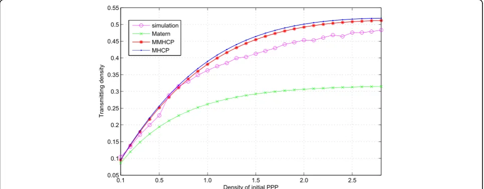
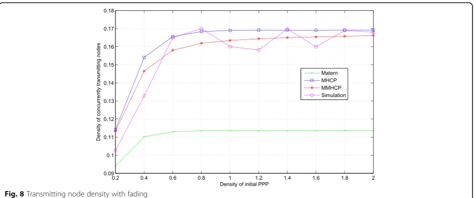
The transmitting node density in a time slot varies with the initial PPP density λpwhenλpis small, but the slope tends to be flat whenλpis large, which is consist-ent with our analysis. And from Figs. 7 and 8, we can see that the slope becomes flat much faster in the pres-ence of fading (whenλp≥0.8 or so) than that in the ab-sence of fading (when λp≥2.5 or so). This concludes that fading makes the transmitting node density tends to be stable much faster. From the figures, the transmitting
Fig. 6Retaining probability with fading
density of MMHCP model is also closer to the simula-tion than the other two models.
In the absence of fading, for the trend of the estimated density following the exclusionre, we take a fixed density of initial PPP as 0.5 and set the exclusion radius from 0.1 to 1, and repeat the simulation for 300 times. The curves are shown in Fig.9, where we can see the trend of trans-mitting density followingre. Meanwhile in the presence of fading, we demonstrate the retaining probability following with the fading parameterμfrom 1 to 10 in Fig.10.
From the analysis in Section 6, we know the mean
probability of successful reception in the models of this paper does not change with the fading parameterμ. We repeat the simulation for 300 times for μ, setting SIR threshold from−5 to 10 dB. The result is shown in Fig. 11. An interesting fact is that the density of initial PPP
has little effect on the e_ps, as illustrated in Fig. 12, which is as same as that in a PPP deployed network.
For transmission capacity, we simulated the impact of the initial PPP density and the fading parameter on the metric. According to the expression of the transmission capacity and the analysis about the probability of successful recep-tion, we know the initial PPP density and fading parameter affect the metric only from the transmitting node density. The Matérn type II model still has the flaw of underestima-tion. An example is shown as Fig.13, that the transmission capacity increases with the density of the potential trans-mitters, where the density of the potential transmitters is set from 0.1 to 1, the fading parameterμis set 10 and the SIR threshold is set 0 dB. Under such a channel condition, we can see that the MMHCP model is closer to the simula-tion result than the MHCP model. Figure14is an example
Fig. 8Transmitting node density with fading
of transmission capacity following with the fading param-eter, where the initial PPP density is set 0.6 and SIR thresh-old is 2 dB. This figure also shows that the simulation is closer to the analysis by MMHCP model.
7.2 Discussions
For the result of transmitting node density of the net-work, it varies little with the initial PPP density, and the underlying reason is intuitive. Whether fading is fixed or not, when the density of initial PPP increases, the retain-ing probability of each node decreases for the character-istic of exclusion in hard core point process. But the transmitting node density of the whole network varies little when the initial PPP tends dense. Here, we take Matérn type II model in fading condition as an example.
The transmitting density can be expressed as
λ1
CSMA¼λp:PMatern¼λp:
1−expð−N~Þ ~
N ¼
1−expð−2πλpΓð2=βÞ
βðP0μ=PtÞ2=βÞ
2πΓð2=βÞ
βðP0μ=PtÞ2=β
. From the
expression, we can see that the density λp only affects the exponent in the numerator, and when it tends to
in-finity, the transmitting density tends to be βðP0μ=PtÞ2=β 2πΓð2=βÞ ,
which tends to be irrelevant toλp.
For the probability of successful reception, we know in a PPP deployed network, it has been proved in [9, 10] that the density of nodes has no impact on the probabil-ity of successful reception. Similarly, in a CSMA net-work deployed by granting hard core points transmitting simultaneously from an initial PPP, we can see from Fig. 12 that the probability e_ps varies little with the initial
Fig. 10Retaining probability withμwith fading
PPP density. From (6), we know that the probabilitye_ps
is affected by λpfrom LI and fr(r). In our analysis, the
retaining probability Pretain decreases with λp, but the product of λpand Pretain actually varies little for a fixed point process. That is why the initial PPP density has lit-tle effect on the final probability of successful reception whenλptends to infinity.
Finally, it should be noted that the reason of MMHCP model outperforming the MHCP model is the network nodes becoming denser or the channel condition be-coming worse. In fact, when the network is sparse and the fading is not so serious, the overestimation of MHCP model is not so obvious, even the intensity underestima-tion flaw still exists in the MHCP, as stated in [20]. That is why the curve of simulation (magenta) is not far from the blue curve (MHCP model) when the fading
parameterμis small (≤6). But with the fading parameter μbecoming large, the curve tends to be close to the red curve (MMHCP model). From this discussion, we know the MMHCP model is more suitable for the dense net-work and with bad fading condition.
8 Conclusions
In this paper, we study the model of dense CSMA net-works with randomly distributed nodes and analyze the transmitting density, mean probability of successful recep-tion, and transmission capacity. In view of that the Matérn type II model underestimates and MHCP model overesti-mates the density of the simultaneously transmitting nodes, we propose another modification on the traditional model to alleviate the overestimation of the density. We give a more accurate density estimation for the
Fig. 12e_psfor different fading factorμwith the SIR
simultaneously transmitting nodes in dense networks and in fading environment. In the absence of fading, given the initial density of the PPP and exclusion radius, we express the density estimation in a closed form by regarding the retaining probability of each node being same. Under Ray-leigh fading condition, we express the retaining probability of a node with fading parameter and initial PPP density. The simulation results demonstrate that the density from MMHCP model is closer to the actual distribution of nodes in CSMA than Matérn type II model and MHCP model. The impact of the density of nodes and fading fac-tor on the mean probability of successful reception and transmission capacity are also studied in our numerical analysis and simulations, from which we can see that the fading parameter has no effect on the probability of suc-cessful reception, which is same as that in the PPP de-ployed network. And the density of initial PPP also has little effect on the probability under Rayleigh fading when the network becomes dense. The density of initial nodes and the fading conditions affect the transmission capacity as they affect the active nodes density, and with the nodes becoming denser or the fading deteriorates, the simulation tends to be close to the MMHCP model. All simulations confirm that the proposed model can be used to accur-ately model the network behavior than Matérn type II and MHCP models in many situations.
Acknowledgements
This work is supported by the NSF of China under Grant 61373027, 61672321, and 61771289 and Shandong Province Higher Educational Science and Technology Program under Grant J15LN06.
Availability of data and materials
All data in this paper are fully available without restriction.
Authors’contributions
YS and RL designed and analyzed the models. YS, HJ, and JZ designed and performed the simulations. YS, RL, and LN wrote the paper. All authors read and approved the final manuscript.
Competing interests
The authors declare that they have no competing interests.
Publisher’s Note
Springer Nature remains neutral with regard to jurisdictional claims in published maps and institutional affiliations.
Author details
1School of Information Science and Engineering, Qufu Normal University, Yantai Road 80, Rizhao 276826, People’s Republic of China.2Department of Computer Science, The George Washington University, Washington, DC, USA. 3College of Computer Science and Technology, Shandong University of Science and Technology, Qingdao 266590, People’s Republic of China. 4Shandong Province Key Laboratory of Wisdom Mine Information Technology, Shandong University of Science and Technology, Qingdao 266590, People’s Republic of China.
Received: 11 October 2017 Accepted: 18 April 2018
References
1. L Feng, J Yu, X Cheng, M Atiquzzaman, A novel contention-on-demand design for wifi hotspots. Pers. Ubiquit. Comput.20(5), 1–12 (2016) 2. L Feng, J Yu, X Cheng, S Wang, Analysis and optimization of delayed
channel access for wireless cyber-physical systems. EURASIP J. Wirel. Commun. Netw.60, 1–13 (2016)
3. M Garetto, T Salonidis, EW Knightly, Modeling per-flow throughput and capturing starvation in csma multi-hop wireless networks. IEEE/ACM Trans. Networking16(4), 864–877 (2008)
4. M Durvy, O Dousse, P Thiran, On the fairness of large csma networks. IEEE Selected Areas in Comm.27(7), 1093–1104 (2009)
5. Y Kim, F Baccelli, G de Veciana, Spatial reuse and fairness in mobile ad-hoc networks with channel-aware CSMA protocols. Int. Symp. Model. Optim. Mob.60(7), 360–365 (2011)
6. G Wang, J Yu, D Yu, H Yu, L Feng, P Liu, Ds-mac: An energy efficient demand sleep mac protocol with low latency for wireless sensor networks. J. Netw. Comput. Appl.58, 155–164 (2015)
7. Q Zhao, T Sakurai, J Yu, L Sun, Maximizing the stable throughput of high-priority traffic for wireless cyber-physical systems. EURASIP J. Wirel. Commun. Netw.2016, 1–12 (2016)
8. H Elsawy, E Hossain, M Haenggi, Stochastic geometry for modeling, analysis, and design of multi-tier and cognitive cellular wireless networks: a survey. IEEE Commun. Surv. Tutorials15(3), 996–1019 (2013)
9. JG Andrews, F Baccelli, RK Ganti, A tractable approach to coverage and rate in cellular networks. IEEE Trans. Commun.59(11), 3122–3134 (2011) 10. H Dhillon, R Ganti, F Baccelli, JG Andrews, Modeling and analysis of k-tier
downlink heterogeneous cellular networks. IEEE J. Sel. Areas Commun. 30(3), 550–560 (2012)
11. S Weber, JG Andrews, N Jindal, An overview of the transmission capacity of wireless networks. IEEE Trans. Commun.58(12), 3593–3604 (2010) 12. V Suryaprakash, J Møller, G Fettweis, On the modeling and analysis of
heterogeneous radio access networks using a Poisson cluster process. IEEE Trans. Wirel. Commun.14(2), 1035–1047 (2015)
13. N Deng, W Zhou, M Haenggi, The Ginibre point process as a model for wireless networks with repulsion. IEEE Trans. Wirel. Commun.14(1), 107–121 (2015)
14. M Haenggi, Mean interference in hard-core wireless networks. IEEE Commun. Lett.15, 792–794 (2011)
15. G Alfano, M Garetto, E Leonardi, New directions into the stochastic geometry analysis of dense csma networks. IEEE Trans. Mob. Comput.13(2), 324–336 (2014)
16. HQ Nguyen, F Baccelli, D Kofman,A Stochastic Geometry Analysis of Dense IEEE 802.11 Networks, Proc. 26th IEEE International Conference on Computer Communications (Infocom 07) (2007), pp. 1199–1207
17. F. Baccelli, B. Blaszczyszyn: Stochastic Geometry and Wireless Networks, Volume II: Applications. Now, Paris (2009). 69–77
18. Y Kim, F Baccelli, G De, Veciana: Spatial reuse and fairness in mobile ad-hoc networks with channel-aware CSMA protocols. IEEE Trans. Information Theory60(7), 360–365 (2011)
19. F Baccelli, B Blaszczyszyn, P Mühlethaler, An aloha protocol for multihop mobile wireless networks. IEEE Trans. Information Theory52(2), 421–436 (2006)
20. H ElSawy, E Hossain, A modified hard core point process for analysis of random csma wireless networks in general fading environments. IEEE Trans. Commun.61(4), 1520–1533 (2013)
21. H. ElSawy, E. Hossain, S. Camorlinga: Characterizing Random CSMA Wireless Networks: A Stochastic Geometry Approach. IEEE ICC 2012- Wireless Networks. Symposium, 5000–5004 (2012)
22. L Ji, S Cheng, Z Cai, J Yu, C Wang, Y Li, Approximate holistic aggregation in wireless sensor networks. ACM transactions on sensor. Networks607(3), 381–390 (2015)
23. Z He, Z Cai, S Cheng, X Wang, Approximate aggregation for tracking quantiles and range countings in wireless sensor networks. Theor. Comput. Sci.13(2), 11–11124 (2017)
24. S Cheng, Z Cai, J Li, Curve query processing in wireless sensor networks. IEEE Trans. Veh. Technol.64(11), 5198–5209 (2015)
25. H He, J Xue, T Ratnarajah, FA Khan, CB Papadias, Modeling and analysis of cloud radio access networks using matérn hard-core point processes. IEEE Trans. Wirel. Commun.15(6), 4074–4087 (2016)
26. A Busson, G Chelius, JM Gorce,Interference Modeling in Csma Multi-Hop Wireless Networks. INRIA, Research. Report, vol 6624 (2008)
27. A Busson, G Chelius,Point Processes for Interference Modeling in CSMA/CA Ad-Hoc Networks, Sixth ACM Symp. Performance Evaluation of Wireless Ad Hoc, Sensor, and Ubiquitous. Networks (2009), pp. 33–40
28. ML Huber, RL Wolpert, Likelihood based inference for matérn type iii repulsive point processes. Adv. Appl. Probab.41(4), 958–977 (2009) 29. J Yu, B Huang, X Cheng, M Atiquzzaman, Shortest link scheduling
algorithms in wireless networks under sinr. IEEE Trans. Veh. Technol.66(3), 2643–2657 (2017)
30. X Zhang, J Yu, W Li, X Cheng, D Yu, F Zhao, Localized algorithms for Yao graph-based spanner construction in wireless networks under sinr. IEEE/ ACM Trans. Networking25(4), 2459-2472 (2017)
31. K Yu, J Yu, X Cheng, T Song,Theoretical Analysis of Secrecy Transmission Capacity in Wireless Ad Hoc Networks, IEEE. Wireless Communications and Networking Conference (2017), pp. 1–6
32. J. Venkataraman, M. Haenggi, O. Collins: Shot Noise Models for the Dual Problems of Cooperative Coverage and Outage in Random. Networks. 44th Annual Allerton Conf. Commun., Control, and Comput., 2642–2650 (2006)
33. J Venkataraman, M Haenggi, O Collins,Shot Noise Models for Outage and Throughput Analyses in Wireless Ad Hoc Networks, Proc. IEEE Military Commun. Conf. (MILCOM 06) (2006), pp. 1–7
34. M Haenggi, RK Ganti, Interference in large wireless networks. Found. Trends Networking3(2), 127–248 (2009)
35. A Hasan, JG Andrews, The guard zone in wireless ad hoc networks. IEEE Trans. Wirel. Commun.6, 897–906 (2007)
36. RK Ganti, F Baccelli, JG Andrews, Series expansion for interference in wireless networks. IEEE Trans. Inf. Theory58(4), 2194–2205 (2012) 37. M Haenggi,Stochastic Geometry for Wireless Networks(Cambridge University