In the present paper we apply a recently developed pattern recognition algorithm SPs to the problem of automated detection of artificial disturbances in one-second magnetic observatory data. TheSPsalgorithm relies on the theory of discrete mathematical analysis, which has been developed by some of the authors for more than 10 years. It continues the authors’ research in the morphological analysis of time series using fuzzy logic techniques. We show that, after a learning phase, this algorithm is able to recognize artificial spikes uniformly with low probabilities of target miss and false alarm. In particular, a 94% spike recognition rate and a 6% false alarm rate were achieved as a result of the algorithm application to raw one-second data acquired at the Easter Island magnetic observatory. This capability is critical and opens the possibility to use theSPsalgorithm in an operational environment.
Key words:Magnetic observatory, magnetogram, spikes, pattern recognition, fuzzy logic.
1.
Introduction
The global network of magnetic observatories is one of the main observation infrastructures for geomagnetic re-search. Magnetic observatory data are used for investi-gating the geomagnetic secular variation originating in the Earth’s outer core, as well as the rapid variations gener-ated by electric currents in the ionosphere, the magneto-sphere and the oceans (e.g., recent papers such as Love, 2008; Matzkaet al., 2010). They are also used by a variety of governmental and industrial customers for applications such as directional drilling, reduction of magnetic survey data and space weather monitoring and forecasting (e.g., Reayet al., 2005; Marshallet al., 2011). Unlike other mag-netometer networks, observatories are aimed at operating for several decades using internationally agreed standards of operations. About 120 observatories currently cooper-ate toward this goal within the INTERMAGNET program (www.intermagnet.org).
One of the main challenges faced by observatories is to being able to provide data of the highest quality on times scales ranging from one second to several decades. Up un-til a few years ago, most INTERMAGNET observatories were producing one-minute filtered data (from measure-ments sampled at a higher frequency, for example every 5 seconds; see St-Louis, 2008). However, in order to address the needs of the space physics community, several observa-tory programs have embarked into a modernization of their equipment in order to being able to produce one-second
fil-Copyright cThe Society of Geomagnetism and Earth, Planetary and Space Sci-ences (SGEPSS); The Seismological Society of Japan; The Volcanological Society of Japan; The Geodetic Society of Japan; The Japanese Society for Planetary Sci-ences; TERRAPUB.
doi:10.5047/eps.2012.03.004
tered data (e.g., Chulliatet al., 2009b; Worthingtonet al., 2009). As expected, the faster measurement sampling rate uncovered various signals that were previously filtered out in one-minute data, including some artificial disturbances that have to be removed from the final observatory data products. While at many observatories the one-second data cleaning represents a reasonable amount of work, it be-comes a daunting task at some observatories, particularly those installed in remote but important locations where no optimal observatory site could be found. For example, it is the case at the recently installed magnetic observatory in Easter Island (Isla de Pascua Mataveri, IAGA code IPM; see Chulliatet al., 2009a and Fig. 1), where the close-by traf-fic of trucks and planes may generate more than hundred artificial disturbances every day.
In the present paper we apply a recently developed pat-tern recognition algorithmSPs(from SPIKEsecond) to the problem of automatically detecting artificial disturbances in one-second magnetic observatory data. The first im-portant step towards automated magnetogram filtering was undertaken by Solovievet al.(2009) and Bogoutdinov et al.(2010). TheSPs algorithm relies on the theory of dis-crete mathematical analysis (Gvishianiet al., 2008a, 2010), which has been developed by some of the authors for more than 10 years. It continues the authors’ research in the mor-phological analysis of time series using fuzzy logic tech-niques (see e.g., Agayan et al., 2005; Gvishiani et al., 2008a, b). We show that, after a learning phase, this al-gorithm is able to distinguish artificial disturbances from natural ones, such as short-period geomagnetic pulsations in the 1 s–1 min period range (e.g., Samson, 1991). This capability is critical and opens the possibility to use theSPs algorithm in an operational environment.
744 A. SOLOVIEVet al.: AUTOMATED DE-SPIKING IN 1 HZ MAGNETIC DATA
Fig. 1. Aerial view of the Isla de Pascua (Easter Island) magnetic observatory. The white, rectangular-shaped magnetometer container is located on the left side of the picture; the absolute hut is about 10 m to its right. Trucks circulating on the dirt road behind the observatory may generate more than hundred spikes per day.
2.
Description of the
SPsAlgorithm
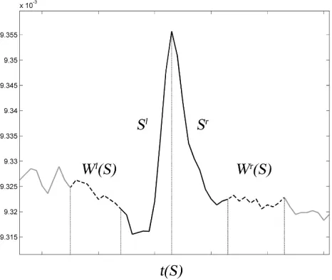
The SPs algorithm is a tool applicable to any time se-ries that has specific time anomalies (disturbances), which have to be identified. The algorithm is aimed at recognition of singular spikes Sof any nature with a simple morphol-ogy on a recordy. (Note thatSPsis not able to recognize jumps; this is done by another algorithm, JM, currently be-ing developed by some of us.) An example of such spike, generated by a nearby running truck, is given in Fig. 2. The logic, which underlies the algorithm, is based on the follow-ing model of a spike. AspikeSis defined as a record frag-ment having atipt(S), where two oppositesharp slopesSl
andSr meet, surrounded byquiet spike wingsWl(S)and
Wr(S)(Fig. 2). In order to formalize the logic of the
algo-rithm, we use the concepts of fuzzy comparison and fuzzy extremality (Zadeh, 1965; Gvishianiet al., 2008a, b). The detailed mathematical description of the algorithm is given in Solovievet al.(2012). In what follows, we provide a brief summary ofSPs.
TheSPsalgorithm consists of three blocks: “-analysis”, “Search for quasi-spikes” and “Selection of spikes” (Fig. 3). The starting recordyis a time seriesy= y(t)given on an interval of discrete positive semiaxisR+h = {t =kh,h > 0,k=1,2, . . .}, wherehis the discretization step andkis the observation node.
The SPs algorithm begins its search by considering a local extremum ofy as a possible tipt = t(S)of a spike S. The algorithm evaluates the slopesSl and Sr on each
side oft. If they turn out to be sharp enough, the triplet S = (Sl,t,Sr), referred to as a quasi-spike, is further
examined. Next, the algorithm searches for quiet wings Wl(S)andWr(S)to the left and to the right of Sl andSr, respectively. If quiet wings are detected, the quasi-spike is recognized as a spike, as defined above. The algorithm is aimed specifically at recognizing such spikes on a recordy. The central part of the algorithm is the “-analysis” (see Fig. 3), which provides a quantitative evaluation of the level of sharpness of slopes and the level of quietness of wings. It also distinguishes “ascending” and “descending” slopes. For a given fragmentky = {y
k, . . . ,yk+}of the record
y, a linear regression (Draper and Smith, 1966) is
calcu-Fig. 2. Illustration of a spikeS(solid black line) consisting of a tipt(S)
and two opposite sharp slopesSl andSr and surrounded by quiet left Wl(S)and rightWr(S)wings (dotted line).
lated by the least-square technique. The regression coeffi-cients are then used to determine whether the fragment is ascending or descending, and to derive an indicator of ac-tivity within the fragment. Determining whether this activ-ity is large (“sharp” fragment) or small (“quiet” fragment) is performed by using fuzzy comparisons (Gvishianiet al., 2008a, b) between a large number of fragments of varying lengths = {1, . . . , m}. InSPs, the following fuzzy
comparison function is used:
nν(A,B)= B−A (Aν+Bν)1/ν,
A≥0, B ≥0, ν >0; nν(0,0)=0
for two numbersAandB, and whereνis a fixed parameter. It yields a number between−1 and 1 which quantifies how muchBis larger thanA.
de-Fig. 3. Block scheme of the algorithmSPs.
scribed classifications and correspondingly identify quasi-spikes and choose genuine quasi-spikes among them.
The algorithm depends on the three free parametersSPs =SPs(ν, ρ1, ρ2)(Fig. 3):
ν—parameter of fuzzy comparison,
ρ1—level of sharpness of the slopesSlandSr,
ρ2—level of quietness of the wingsWl(S)andWr(S).
A given set of free parameters is denoted by π = (ν, ρ1, ρ2).
3.
Testing Dataset and Methodology
746 A. SOLOVIEVet al.: AUTOMATED DE-SPIKING IN 1 HZ MAGNETIC DATA
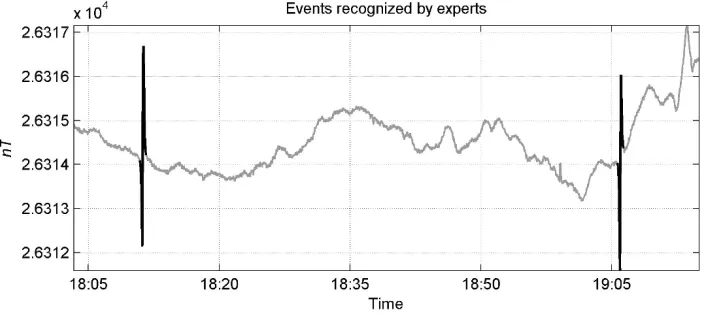
Fig. 4. Examples of artificial spikes removed after manual recognition (Xcomponent, 5 July 2009). Recognized spikes are marked with black.
Fig. 5. Example of geomagnetic pulsations (Xcomponent, 1 July 2009).
Table 1. Statistical information on spikes from 01/07/2009 to 20/07/2009 recognized by eye on magnetograms.
Channel Number of Min Max Mean Min Max Mean
spikes amplitude, amplitude, amplitude, duration, duration, duration,
nT nT nT s s s
X 1119 0.100 82.280 1.298 9 190 27.330
Y 1122 0.080 100.340 1.093 4 190 27.193
Z 996 0.100 20.640 0.371 6 470 28.861
F 1135 0.102 61.770 0.918 9 439 31.719
Table 2. Statistical information on spikes from 21/07/2009 to 31/07/2009 recognized by eye on magnetograms.
Channel Number of Min Max Mean Min Max Mean
spikes amplitude, amplitude, amplitude, duration, duration, duration,
nT nT nT s s s
X 853 0.100 12.630 1.200 7 449 26.917
Y 844 0.140 12.430 0.972 9 449 27.096
Z 774 0.090 106.510 0.570 7 449 27.722
F 846 0.088 61.130 0.932 6 449 31.072
data points.
The testing dataset was entirely cleaned using standard observatory tools; i.e., spikes caused by trucks, planes and other artificial sources were manually removed after a de-tailed inspection of daily magnetograms. Figure 4 shows examples of such spikes. They have a characteristic shape, which makes them easily recognizable by eye. However,
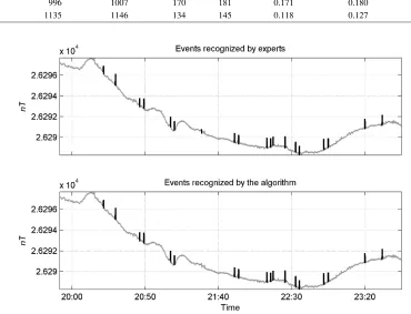
Fig. 6. Comparison between algorithm (bottom) and manual (top) recognition results (Xcomponent, 1 July 2009). In both cases recognized spikes are marked with black.
estimation of spike amplitudes and durations, is given in Tables 1 and 2.
The first part of the testing dataset, from 1 to 20 July 2009, was used for the training of the algorithm. As can be seen in Table 1 the mean spike amplitude vary from one channel to the next, and therefore we performed algorithm learning for each channel X, Y, Z, F separately. As a result, we were able to obtain the optimal free parameter values of the algorithm for each channel independently. In order to select optimal values of free parameters, we implemented a brute-force search, i.e., we systematically tried a large number of values (Knuth, 1968). First, each 1-day 1-channel data series was processed by the algorithm using the following set of free parameter values:
=
ν =0.4,0.5,0.6,0.7;
ρ1=0.45,0.5,0.55,0.6,0.65;
ρ2=0.2,0.25,0.3,0.35,0.4
.
These values were pre-selected based upon the known be-havior of the fuzzy comparison function and some prelimi-nary tests. In total,|| =100 combinations of free parame-ters were tested. To assess recognition quality we introduce the following function to be minimized:
Kλ(SPs(π))=λP1(SPs(π))+(1−λ)P2(SPs(π)),
whereSPs(π)is a result of the algorithm operation with some combination of free parameter valuesπexpressed in a set of intervals on the time axis, which define recognized events; P1 is the probability of thefirst kind error (target
miss) defined as Nmissed
Neye (where N is the number of spikes); P2 is the probability of the second kind error (false alarm)
defined as Nfalse
Nalgorithm; 0≤ λ ≤ 1 (Bogoutdinovet al., 2010).
In the criterionKλwe putλ=0.8, thus expressing a higher degree of importance of not missing spikes versus avoiding false alarms. The value of the parameterλ was obtained by testing the algorithm for λ = 0.1,0.2, . . . ,0.9 on an arbitrary set of free parameters and selecting the value for which the best recognition was achieved.
one-748 A. SOLOVIEVet al.: AUTOMATED DE-SPIKING IN 1 HZ MAGNETIC DATA
Fig.
7.
Examples
of
spik
e
recognition
by
the
algorithm
SPs
(
X
component,
1
July
2009).
Recognized
spik
es
are
mark
ed
with
recognized recognized by spikes events of an error of an error criterion
by eye the algorithm of the 1st kind of the 2nd kind K0.8
X 2122 2057 79 14 0.0372 0.0068 0.031
Y 2143 2150 23 30 0.0107 0.0140 0.011
Z 1786 1780 104 98 0.0582 0.0551 0.058
F 1963 1996 39 72 0.0199 0.0361 0.023
second data.
Once the free parameters werefixed, wefirst tested the algorithm by applying it to the time interval from 21 to 31 July 2009 and comparing with the results of manual data cleaning. By separating the dataset in two parts, we thus made sure that the testing was performed on an independent dataset. Next, we applied the algorithm to the time interval from 1 to 31 August 2009 and then performed recognition of spikes by eye in order to check the results.
4.
Results
4.1 Results of the learning phase
The following optimal free parameter values were found to give the best results for the overall criterion of recogni-tionK0.8for each channel:
The overall numbers of target misses and false alarms as well as the values of the recognition criterion for each com-ponent are provided in Table 3. The best results of the algo-rithm learning were achieved in the case of the horizontal components X andY, where the error probabilities varied between 3.5% and 11.5%. Less good results were obtained in the case of the vertical component Z, where the error probabilities of thefirst and the second kinds were 17.1% and 18.0% correspondingly. This difference is attributed to the smaller average amplitude of the spikes on theZ com-ponent during the learning phase time interval, which made them more difficult to detect.
Some screenshots illustrating application results of the algorithmSPs=SPs(πX∗)are given in Figs. 6 and 7.
4.2 Results of the testing phase
The results of the testing phase are provided in Table 4. Comparison of recognition results obtained on data for 1– 20 July (learning material) and 21–31 July (testing material)
shows that the recognition quality is about the same. For-mally it is confirmed by very close values of the calculated quality criterion (Tables 3, 4). It can be concluded that the overall recognition performance achieved during the learn-ing phase could be reproduced durlearn-ing the testlearn-ing phase.
4.3 Results of the blind test
The blind test involved data recorded from 1 to 31 Au-gust 2009 with noa priori expert opinion. The results of the recognition by the algorithmSPs=SPs(π∗)were sub-sequently evaluated by eye. The overall recognition statis-tics for the whole set of data are provided in Table 5.
The probability of missed spikes for the X component is 3.72%, that of false alarms is 0.68%, to be compared with 4.7% of missed spikes and 8.7% of false alarms for the 1/07–20/07 time interval (Table 3) and 5.9% of missed spikes and 6.0% of false alarms for the 21/07–31/07 time interval (Table 4). In the case of the other componentsY,Z and the total intensity F the blind test also demonstrated higher efficiency of the algorithm application comparing to results of learning and testing phases, which is well re-flected in the corresponding values ofK0.8quality criterion
(Tables 3–5).
The difference in algorithm recognition qualityK0.8
ob-tained for records for August and July 2009 is likely due to the fact that it was easier to carry out manual data process-ing by eye havprocess-ing at the disposal the results of the algorithm recognition (August data), rather than to analyze raw mag-netograms“from scratch”(July data). Thus for July data the quality of manual recognition of spikes turned to be worse. This shows that the algorithm significantly helped the recognition by eye. It also provides some estimate of the amount of errors made when relying on manual spike detection.
in-750 A. SOLOVIEVet al.: AUTOMATED DE-SPIKING IN 1 HZ MAGNETIC DATA
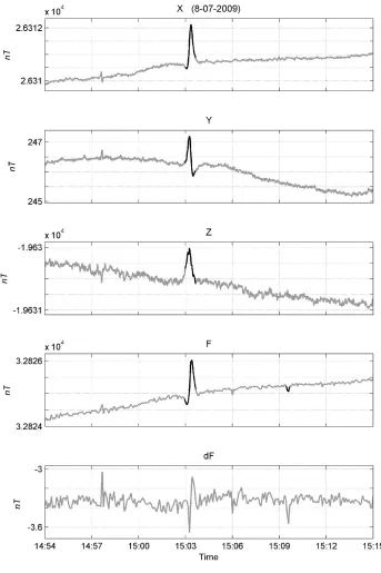
Fig. 8. Example of“false spike”seen ond Frecord (bottom) on the left. Spikes recognized by eye on initial recordsX,Y,ZandFare marked on the corresponding records with black. The“false spike”seen ond Frecord could be representative of low amplitude spikes onX,Y,ZandFrecords and therefore less visible in the background noise of theX,Y,ZandFrecordings.
tervals not caused by trucks or airplanes.
The results of the blind test confirm that the learned al-gorithm is able to detect most of the spikes, and shows that there is some variability from one day/week/month to the next.
5.
Discussion
In the present paper we introduced the algorithm SPs, able to automatically recognize spikes caused by artifi -cial disturbances in magnetic observatory data sampled ev-ery second. We applied this algorithm to the recently in-stalled observatory in Easter Island, where nearby trucks
and planes cause several tens of such spikes every day. We showed that, after a 20-day learning phase in July 2009, the algorithm is able to recognize more than 94% of the spikes on the three components and the intensity recordings in Au-gust 2009, while the percentage of false alarms is less than 6%. At all the stages the algorithm showed worse results in processing vertical componentZ.
Fig. 9. Example of a spike absence ond Frecord (bottom) on the right. Spikes recognized by eye on initial recordsX,Y,ZandFare marked on the corresponding records with black.
the simultaneous occurrence of a pulsation-like signal at a nearby observatory. This functionality is not included in the present version of the algorithm. In some rare cases, false alarms are due to the temporary increase of the background noise, whose origin is unknown.
A standard method to detect spikes in magnetic observa-tories consists in taking the differenced F = Fs−Fv
be-tween thefield modulusFs = F directly measured by the
scalar magnetometer and that Fv calculated from the three
components measured by the vector magnetometer. Nor-mally,d Fshould vary by a up to a few tenths of nT around a constant non-zero value due to the differences in trans-fer functions and locations of the instruments. Instrumental
752 A. SOLOVIEVet al.: AUTOMATED DE-SPIKING IN 1 HZ MAGNETIC DATA
Another disadvantage ofd Fmethod is that it needs pres-ence of both vector data on the three components and scalar data on totalfield intensity and consequently correct oper-ation of the both devices is required. The method becomes invalid if one of the devices doesn’t work properly or regis-tration of one of the three vector components is failed. On the contrary, datafiltration using theSPsalgorithm can be applied to any particular record regardless of the presence of other records. It makes the algorithm applicable not only at magnetic observatories but also at magnetic stations where only variational data registration is carried out.
We plan to carry out further studies on seasonal and ac-tivity level dependence of the recognition results. The de-scribed algorithm is currently being implemented in the op-eration of the Russian-Ukrainian geomagnetic data center hosted by the Geophysical Center of the Russian Academy of Sciences. The development of a web application based upon theSPsalgorithm is also being considered, in order to make it available to the wider magnetic observatory com-munity.
Acknowledgments. We thank Alan W. P. Thomson and Hans-Joachim Linthe for constructive reviews. The research has been carried out in the framework of collaboration program between In-stitut de Physique du Globe de Paris (IPGP), Moscow InIn-stitute of Physics of the Earth of Russian Academy of Sciences (IPE RAS) and Geophysical Center of RAS (GC RAS). The development of the algorithmSPshas been carried out in the framework of the project number 12-05-90428 supported by Russian Foundation for Basic Research. The Easter Island (IPM) magnetic observatory is jointly operated by Direccion Meteorol´ ogica de Chile (DMC) and´
IPGP. We thank INTERMAGNET for promoting high standards of magnetic observatory practice (www.intermagnet.org). This is IPGP contribution number 3288.
References
Agayan, S. M., S. R. Bogoutdinov, A. D. Gvishiani, E. M. Graeva, J. Zlotnicki, and M. V. Rodkin, Study of signal morphology basing on fuzzy logic algorithms,Geophys. Res. Proc. Moscow, IPE RAS,1, 143– 155, 2005 (in Russian).
Bogoutdinov, S. R., A. D. Gvishiani, S. M. Agayan, A. A. Solovyev, and E. Kihn, Recognition of disturbances with specified morphology in time series. part 1: spikes on magnetograms of the worldwide INTERMAG-NET network,Izv. Phys. Solid Earth,46(11), 1004–1016, 2010. Chulliat, A., X. Lalanne, L. R. Gaya-Piqu´e, F. Truong, and J. Savary, The
new Easter Island magnetic observatory, inProceedings of the XIIIth IAGA Workshop on Geomagnetic Observatory Instruments, Data Ac-quisition and Processing, edited by J. J. Love, 271 pp., U.S. Geological Survey Open-File Report 2009-1226, 2009a.
Chulliat, A., J. Savary, K. Telali, and X. Lalanne, Acquisition of 1-second
data in IPGP magnetic observatories, inProceedings of the XIIIth IAGA Workshop on Geomagnetic Observatory Instruments, Data Acquisition and Processing, edited by J. J. Love, 271 pp., U.S. Geological Survey Open-File Report 2009-1226, 2009b.
Draper, N. R. and H. Smith,Applied Regression Analysis, 407 pp., Wiley, New York, 1966.
Gvishiani, A. D., S. M. Agayan, Sh. R. Bogoutdinov, J. Zlotnicki, and J. Bonnin, Mathematical methods of geoinformatics. III. Fuzzy compar-isons and recognition of anomalies in time series,Cybern. Syst. Anal.,
44(3), 309–323, 2008a.
Gvishiani, A. D., S. M. Agayan, and Sh. R. Bogoutdinov, Fuzzy recog-nition of anomalies in time series,Dokl. Earth Sci.,421(5), 838–842, 2008b.
Gvishiani, A. D., S. M. Agayan, S. R. Bogoutdinov, and A. A. Soloviev, Discrete mathematical analysis and geological and geophysical applica-tions,Vestnik KRAUNZ. Earth Sciences, 2,16, 109–125, 2010 (in Rus-sian).
Knuth, D.,The Art of Computer Programming. Volume 3: Sorting and Searching, 800 pp., Addison-Wesley, USA, 1968.
Love, J. J., Magnetic monitoring of Earth and space,Phys. Today,61, 31– 37, 2008.
Marshall, R. A., E. A. Smith, M. J. Francis, C. L. Waters, and M. D. Sciffer, A preliminary risk assessment of the Australian re-gion power network to space weather, Space Weather, 9, S10004, doi:10.1029/2011SW000685, 2011.
Matzka, J., A. Chulliat, M. Mandea, C. Finlay, and E. Qamili, Geomag-netic observations for mainfield studies: from ground to space,Space Sci. Rev.,155, 29–64, doi:10.1007/s11214-010-9693-4, 2010. Reay, S. J., W. Allen, O. Baillie, J. Bowe, E. Clarke, V. Lesur, and S.
Macmillan, Space weather effects on drilling accuracy in the North Sea,Ann. Geophys.,23, 3081–3088, doi:10.5194/angeo-23-3081-2005, 2005.
Samson, J. C., Geomagnetic pulsations and plasma waves in the Earth’s magnetosphere, inGeomagnetism. Vol. 4, edited by J. A. Jacobs, 481– 592, 825 pp., Academic Press, London, 1991.
Soloviev, A. A., Sh. R. Bogoutdinov, S. M. Agayan, A. D. Gvishi-ani, and E. Kihn, Detection of hardware failures at INTERMAG-NET observatories: Application of artificial intelligence techniques to geomagnetic records study, Russ. J. Earth Sci., 11, ES2006, doi:10.2205/2009ES000387, 2009.
Soloviev, A. A., S. M. Agayan, A. D. Gvishiani, S. R. Bogoutdinov, and A. Chulliat, Recognition of disturbances with specified morphology in time series. Part 2: Spikes on 1-second magnetograms,Izv. Phys. Solid Earth, 2012 (accepted).
St-Louis, B.,INTERMAGNET Technical Reference Manual, Version 4.4, 86 pp., 2008.
Worthington, E. W., E. A. Sauter, and J. J. Love, Analysis of USGS one-second data, inProceedings of the XIIIth IAGA Workshop on Geomag-netic Observatory Instruments, Data Acquisition and Processing, edited by J. J. Love, 271 pp., U.S. Geological Survey Open-File Report 2009-1226, 2009.
Zadeh, L. A., Fuzzy sets,Inf. Control.,8, 338–353, 1965.