On the statistical convergence of bias in mode based Kalman filter for switched systems

R E S E A R C H

Open Access

On the statistical convergence of bias in

mode-based Kalman filter for switched systems

Wenji Zhang

and Balasubramaniam Natarajan

Abstract

Many physical and engineered systems (e.g., smart grid, autonomous vehicles, and robotic systems) that are observed and controlled over a communication/cyber infrastructure can be efficiently modeled as stochastic hybrid systems (SHS). This paper quantifies the bias of a mode-based Kalman filter commonly used for state estimation in SHS. The main approach involves modeling the bias dynamics as a transformed switched system and the transitions across modes are abstracted via arbitrary switching signals. This general model effectively captures a wide range of SHS systems where the modes may follow deterministic, Markovian, or guard condition based transitions. By leveraging techniques developed to analyze the stability of switched systems, we derive conditions for statistical convergence of the bias in a mode-based Kalman filter in the presence of mode mismatch errors. Developed upon the foundations of Lyapunov theory, we demonstrate a linear matrix inequality condition that guarantees asymptotic stability of the corresponding autonomous switched system irrespective of the choice of mode mismatch probability. Furthermore, we obtain the range of mode mismatch probabilities that assures bounded input bounded output stability of the bias dynamics for both stable and unstable SHS. Using numerical simulations of a smart grid with network topology errors, we verify and validate the theoretical results and demonstrate the potency of using the analysis in critical

infrastructures.

Keywords: Kalman filter, Stochastic hybrid system, Error analysis

1 Introduction

Stochastic hybrid systems (SHS) represent a class of dynamical systems that experience interactions of both discrete and continuous dynamics with uncertainty. The uncertainty can be modeled in continuous dynamics, discrete state transitions, or both. In most cases, the evolution of continuous state is described via stochastic differential/difference equation (SDE) whereas the dis-crete state evolves depending on the application. Typi-cal examples include random process (such as Markov chain) and guard conditions (i.e., the discrete state tran-sitions depend on the continuous state). The first type of SHS has been applied in modeling of biochemical processes [1, 2], manufacturing processes [3], and com-munication networks [4]. The second type of SHS, also known as state-dependent SHS, finds application in flight management systems [5, 6]. For more complex systems

*Correspondence:[email protected]

Department of Electrical and Computer Engineering, Kansas State University, 1701D Platt St., Manhattan 66506, KS, USA

such as a microgrid [7], the transitions of discrete state may be governed by both random processes and guard conditions.

1.1 Motivating example: impact of smart grid network topology error

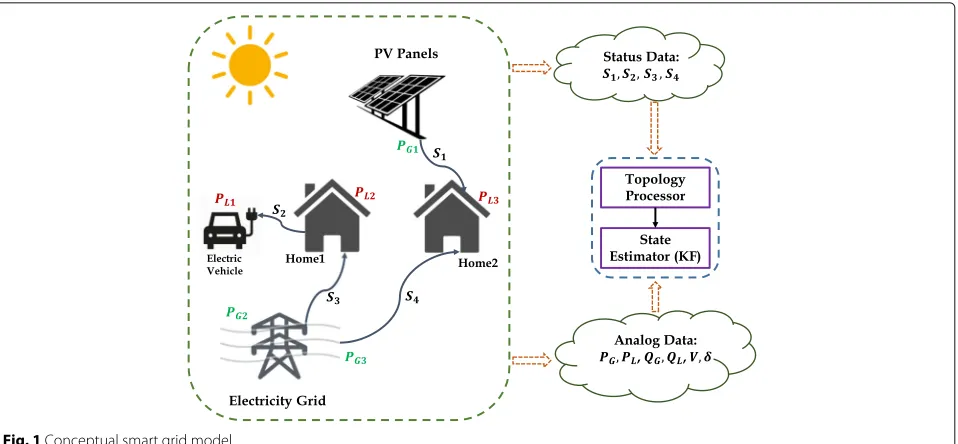
Our conventional power grid is transitioning to a “smart grid” with the addition of renewable energy source (e.g., photovoltaics (PV)), advanced metering and sensing infrastructure, electric vehicles, and controllable loads [7]. A conceptual small-scale smart grid model is shown in Fig.1. This toy model includes a bank of PV panels, elec-tricity grid, home loads, and electric vehicles.S1, S2, S3,

andS4are switches whose status determine the network

topology. In practice,S2can be switched OFF when

peo-ple unplug their electric vehicles and S1, S3, andS4can

be switched ON or OFF based on power demand and the weather. To aid state estimation in a smart grid, there are typically two types of data collected [8]:

Fig. 1Conceptual smart grid model

1 Status data for switches, breakers, and communication links. Status data defines the real-time network topology of the grid.

2 Analog data such as bus voltage, power flow, and reactance. Analog data is used to determine the voltage profile at different nodes of the power grid.

In general, a smart grid can be formally modeled as an SHS with each switch status determining a specific network topology (discrete state) and continuous state capturing the analog parameter dynamics. A typical estimator for the continuous dynamics is a mode-based Kalman filter [9–17] which relies on mode information. Discrete mode information may be obtained from status data entered by human operators or sensor measurements or esti-mated based on measurements. These approaches are error prone due to human errors, missing data, communi-cation, or estimation errors. Consequently, errors in status data result in network topology errors which eventually lead to performance degradation in a mode-based Kalman filter. In this work, we explore the impact of discrete state estimation error (or inaccurate information) on the quality of continuous state estimation derived via a mode-based Kalman filter.

1.2 Related work

State estimation in SHS has attracted research interest for decades. Kalman filter-based solutions dominate the arena. For one category of SHS where both discrete and continuous states are observable and the discrete state transitions are independent with continuous state, mode-based Kalman filter can be applied as a minimum mean square error (MMSE) estimator [10–12]. Matei et al. [13]

proposes a Kalman filter-based MMSE estimator for SHS with observation of continuous state and delayed mea-surement of discrete state. Matei and Baras [14] expand their results to the case of delayed observations of both continuous and discrete states. In general SHS appli-cations, discrete state may not be directly observable [12,15–21]. In this case, the optimal estimator is obtained from a weighted sum of a bank of Kalman filters with each matched to a possible mode. Therefore, it requires expo-nentially increasing memory and computing time. A cou-ple of hybrid estimation algorithms have been proposed for Markov jump linear system (MJLS), such as interacting multiple model (IMM) algorithm [19] and multiple model adaptive estimation (MMAE) algorithm [20,21]. Seah and Hwang [15] and Liu et al. [16] extend the IMM algorithm to state-dependent SHS. Note that all the abovementioned algorithms require online computation with a bank of Kalman filters and they suffer from high computational complexity. Zhang and Natarajan [17]and Hofbaur et al. [18] decrease the complexity by formulating the mode estimation as a problem of belief-state update and using only one Kalman filter corresponding to estimated mode for continuous state estimation.

exponentially increasing memory and computing time. Another option is to treat the known discrete state as the true state and conduct estimation via only one Kalman filter. This Kalman filter is optimal if there is no mode mismatch. In case of a mode mismatch, the resulting estimator will be biased. Review of the recent literature reveals that there is limited prior work that considers the bias of a mode-based Kalman filter in SHS estimation. For non-hybrid scenarios, Kalman filter is proved to be an unbiased estimator. Therefore, multiple papers have analyzed the performance of Kalman filters by only focus-ing on error covariance [22–30]. Specifically, [22–28,30] consider dynamical system with missing measures, inter-mittent observations, random delays, and packet dropouts and they follow the similar approach of deriving a bound for the critical probability of missing observation that ensures the convergence of error covariance. Another work [31] considers an estimation problem where the model for the Kalman filter is mismatched with the true system. Unlike the previous mentioned papers, [31] stud-ies the residual of Kalman filter and derives mean and covariance of the Kalman filter residual without analyzing its convergence behavior. In terms of estimation strate-gies for SHS, there have been several prior efforts [32–35]. Their analysis is based on MMAE algorithm and the IMM approach. Hwang et al. [32] first consider the problem of quantifying performance of a hybrid estimation algorithm and derive the condition for exponential convergence of the estimator in terms of detection delay and sojourn time [33]. In [34,35], the authors extend their research on eval-uating the stability of IMM algorithm and they focus on the mean and covariance of the Kalman filter residual. However, the existing research efforts have not explored the relationship between mode mismatch error and SHS estimation. It is not known as to how discrete state esti-mation error influences the performance of a mode-based Kalman filter. How sensitive is the convergence of bias in a mode-based Kalman filter to errors in discrete state knowledge? Is there a critical region within which the error dynamics in a mode-based Kalman filter will con-verge? These are the fundamental unanswered questions that our work seeks to address.

1.3 Contributions

In this paper, we study the statistical convergence of the bias dynamics in a mode-based Kalman filter in the pres-ence of mode mismatch errors. To our best knowledge, our work is the first attempt to quantify the influence of inaccurate mode information on continuous state estima-tion process. Specifically, we consider a linear SHS frame-work that finds application in many practical system, e.g., smart grid and aircraft management system. In our previ-ous work [36], we derived the dynamics of bias that results from mode mismatch errors for a specific model of SHS

with two discrete states. Additionally, the discrete state transitions were modeled via independent and identically distributed (i.i.d) binary Bernoulli random variables. For this specific system, we derived the sufficient condition for statistical convergence of bias. In contrast to the con-ference paper, the assumptions of two modes and i.i.d. Bernoulli transitions are relaxed in this work. The exten-sion is not trivial because for SHS with two modes, there is only one error mode for a given discrete state. There-fore, in this work, we take a fresh perspective and propose to use a transformed switched system to describe the bias dynamics. The convergence of the bias is then mapped to the stability of the transformed switched system. The SHS model considered in this paper is general and can be applied to many practical systems. The novelty of this work lies in modeling the bias dynamics as a transformed switched system enabling us to exploit techniques devel-oped for stability analysis of switched system to our prob-lem of interest. Specifically, the stability analysis involves two stages. First, we consider stability of the correspond-ing autonomous switched system and derive sufficient and necessary conditions that guarantee asymptotic stability. Second, we investigate the bounded input bounded out-put stability and acquire a tolerant region on probability of mode mismatch errors that guarantees the convergence of the bias dynamics. The boundedness of the input is related to the stability of the original SHS and we consider both stable and unstable cases. Finally, the theoretical results are verified and validated using numerical simulations of a smart grid with network topology errors. Theoretical and numerical results help us identify the fidelity required in discrete state knowledge in order to meet the performance requirements of continuous state estimates.

The rest of the paper is organized as follows: The system model, mode-based Kalman filter, and its performance metrics are introduced in Section 2. In Section 3, we derive the bias dynamics and the model of a transformed system that fully captures the bias evolution. The stabil-ity analysis for the transformed system is discussed in Section4. The stability conditions and tolerant region for mode mismatch error are also derived as the main results in Section4. Two experiments are conducted, and the sim-ulation results are presented in Section4. We conclude this work and discuss future directions in Section6.

2 Preliminaries

2.1 Notations

and inverse of a matrix, respectively. For any vector u, u[i] denotesith element of the vector. For a symmetric matrix A, A0 denotes that A is positive definite and A≺0 indicates thatAis negative definite.E(·)represents expectation andP(·)represents probability measure.

2.2 System model

We consider a discrete-time autonomous linear SHS. Mathematically, the continuous statexk ∈ Rnand

mea-surementyk ∈Rmare related via the following equations:

xk =Aqkxk−1+Bqkwk,

yk =Cqkxk+vk. (1)

Here,qk ∈Qrepresents the discrete state at timek, which

is sometimes referred to as the mode. Without loss of gen-erality, we define Q = {1, 2, 3,. . .,d}. For eachq_k, the correspondingAqk is ann-by-nmatrix,Bqk is ann-by-p

matrix, andCqk is am-by-nmatrix. Regarding the system

model, we have the following assumptions:

1 wk∼N(0,Q)andvk ∼N(0,R)are mutually independent white Gaussian capturing model and measurement uncertainty, respectively.

2 The initial distribution of the continuous state

follows a Gaussian distribution . The

discrete state has a unique initial modeq0∈Q. 3 For allq_k ∈Q,Aqk,BqkQBqk

is controllable and

Cqk,Aqk

is observable.

In this paper, we consider a generalized SHS model without restricting ourselves to any specific type of dis-crete state transitions. At a higher level, the generalized SHS can be astracted as a switched system with arbitrary switching. This allows us to neglect specific details of the discrete state behavior and instead incorporate all possi-ble switching patterns [37]. With this connection between switched system and the generalized SHS model in mind, we confine ourselves to the convention of switched sys-tems with arbitrary switching signals throughout the remainder of this paper.

As an illustrative example, we consider a toy smart grid setup inspired by [7, 38]. The system consists of three components—main distribution grid, local power net-work, and electrical loads. The discrete status for each component is:

• Local power network—On: 1, Failure mode: 0; • Distribution grid (G )—Connected: 1, Disconnected:

0;

• Electrical loads (D )—Connected: 1, Disconnected: 0.

The corresponding power generation and power con-sumption dynamics are given below:

• Grid power: If the micro grid is connected to the main electricity grid (G=1), the grid powerPGhas the following dynamics:P˙G=kGPG+σGdW, where kGis a proportional coefficient andσGis a variation parameter [7]. IfG=0, bothkGandσGare close to 0.dW denotes Wiener process.

• Electrical loads: Electrical loads can be modeled via a stochastic differential equation. We use Uhlenbeck-Ornstein model to describe electricity loads [38]. Let

˙

PD=α(m−PD)dt+σDdW. Here, we assumem=0.

αrepresents a tracking coefficient.σDis a variation coefficient, anddW denotes Wiener process.

Therefore, the continuous state in this smart grid system can be defined asx =[PG,PD] with corresponding state

equation as:

_˙

PG ˙

PD

=

kG 0

0 −α PG PD

+

σG 0

0 σD

dW dt .

By discretizing the state space with a sampling period ofτ, we get a discrete-time SHS:

xk =Aqkxk−1+Bqkwk, (2)

where

Aqk =

ekGτ ₀

0 e−ατ

, (3)

and

Bqk =

kG 0

0 −α −1

(Aqk−I)

σG 0

0 σD

. (4)

Here, the indexkcorresponds to the time instantkτ. The discrete state space is defined by combination of different status ofL,G, andD. Consequently, the value of parame-terskG,α,σG, andσDare determined by different discrete

states. The measurement equation corresponds to

yk=Cqkxk+vk. (5)

We will provide more details on this smart grid model in Section5.2.

2.3 Mode-based Kalman filter

The goal of a mode-based Kalman filter is to estimatexk

based on knowledge of discrete states qˆk and

measure-mentsyk until timek. Note that the known modeqˆkcan

be inconsistent with the true modeqkresulting in a mode

mismatch error. Denote the measurement sequence and known mode sequence up to timekasys_k = (y1,· · ·,yk)

and qˆs_k = (qˆ1,· · ·,qˆk), respectively. The mode-based

Algorithm 1Mode-based Kalman filter

1: functionESTIMATION UPDATE(μμμ₀,M0|0,Q,R,qˆs_k,ysk)

2: x0|0=μμμ0,M0|0=0

3: ys_k=(y1,· · ·,yk)

4: qˆs_k =(qˆ1,· · ·,qˆk)

5: fori=1 :kdo 6: xi|i−1=Aqˆixi−1|i−1

7: Mi|i−1=AqˆiMi−1|i−1A_qˆ_i+BqˆiQB_qˆ_i

8: Kqˆi,i=Mi|i−1C_qˆ_i(CqˆiMi|i−1C_qˆ_i+R) −1

9: xi|i=xi|i−1+Ki,qˆi(yi−Cqˆixi|i−1)

10: Mi|i=(I−Ki,qˆiCqˆi)Mi|i−1

11: end for 12: return xk|k

13: end function

Here,K_qˆi,iis the Kalman gain related to modeqˆi.xk|kis

the estimate ofxk, and we denote it asxˆk. If the

estima-tor has full knowledge of the actual mode, i.e.,qˆs_k = qs_k, then the mode-based Kalman filter has been proven to be an unbiased minimum mean square error estimator. However,qˆs_k = qs_k does not always hold in practice. As a consequence, the inconsistency betweenqs_kandqˆs_kresults in a bias in the mode-based Kalman filter estimate. In the following, we will first derive the formulation of bias dynamics and then discuss its statistical convergence.

2.4 Bias dynamics in the presence of mode mismatch

In general, the bias is defined as the difference between the estimator and the actual value of a state. However, for a mode-based Kalman filter, bothxˆk andxk are

ran-dom variables which result in the bias being a ranran-dom variable. Therefore, we define the bias to be the differ-ence between means of estimator and the true state, i.e., ek =E(xˆk)−E(xk). In other words, we capture the

differ-ence betweenxˆkandxkin a mean sense viaek. This metric

is similar to those considered in [31,32]. Based on Algo-rithm 1, we derive the bias dynamics in a Kalman filter due to mismatch betweenqs_kandqˆs_k.

Theorem 1Given the actual mode sequence qs_k = (q1,· · ·,qk) and estimated mode sequence qˆsk =

(qˆ1,· · ·,qˆk), the bias dynamics in a mode-based Kalman filter corresponds to:

ek =

A_qˆk−K_qˆk,kCqˆkAqˆk

ek−1

+A_qˆk−K_qˆk,kCqˆkAqˆk +Kqˆk,kCqkAqk−Aqk

E(xk−1).

ProofThe expectation ofxkis:

E(xk)=E(E(xk|xk−1))=AqkE(xk−1).

The stochasticity of the estimate xˆk comes from the

randomness in the measurements. Therefore, we can write the mean ofxˆkas:

E(xˆk)=E(E(xˆk|ˆxk−1))=AqˆkE(xˆk−1) +Kqˆk,k(E(yk)−CqˆkAqˆkE(xˆk−1)).

From the definition of biasek, we have:

ek=E(xˆk)−E(xk) =Aqˆk−Kqˆk,kCqˆkAqˆk

Exˆk−1

+Kqˆk,kCqkAqk −Aqk

Exk−1

Substituting forE(xˆk−1)=ek−1+E(xk−1), we get:

ek=

A_qˆk−K_qˆk,kC_qˆkA_qˆk ek−1+E

xk−1

+K_qˆk,kCqkAqk−Aqk

Exk−1

=A_qˆk −K_qˆk,kC_qˆkA_qˆkek−1

+A_qˆk−K_qˆk,kC_qˆkA_qˆk+K_qˆk,kCqkAqk−Aqk

Exk−1

.

For the sake of compactness in notation, we introduce

t and i to denote actual mode and estimated mode at time k. That is, t = qk ∈ Q and i = ˆqk ∈ Q. It

needs to be noted that t andi are indeed time-variant random variables. With this, the evolution ofek can be

rewritten as:

ek =(Ai−Ki,kCiAi)ek−1

+(Ai−Ki,kCiAi+Ki,kCtAt−At)E(xk−1).

For each modei, letKi be the steady state Kalman gain. Since we assume thatQandRare the same for all modes

i ∈ Q, the Kalman gainKi,k will converge to the

corre-sponding steady Kalman gainKi quickly [9]. Therefore, the update ofekcan be approximately written as:

ek=(Ai−KiCiAi)ek−1+(Ai−KiCiAi+KiCtAt−At)E(xk−1).

(6)

Denotei=Ai−KiCiAi,i,t=At−KiCtAt, whent=i, i,t=i. In general,

ek =iek−1+(i−i,t)E(xk−1). (7)

In the following sections, we will model the evolution of ekas a transformed switched system and further leverage

results in stability analysis for switched systems to derive our main results.

3 Transformed switched system

So far, we have derived the dynamics of the bias in a mode-based Kalman filter. In Eq. (7), the bias evolves mode-based on matricesiandi,t. As defined in the previous section,i

t, there ared−1 mode mismatch errors that could hap-pen. Intuitively, we want to derive the evolution of ek

as a stochastic equation based on the probabilistic event of mode mismatch occurrence. In the following, we will formally model this random process by introducing two sequences of random variables,{t}tt==d1and{t}tt==d1as:

abilityλi,t can be interpreted as the probability that the estimated mode isiwhile the true mode ist. It is worth mentioning that in realistic applications, the probability of mode mismatch may not only be a function ofiandt

but can also be correlated across time or across modes. Similarly, a random variabletis defined as:

t=

Note that the probabilities are the same astfor the same

t. Withtandt, we can rewrite Eq. (7) as:

ek=tek−1+tE(xk−1). (8)

From Eq. (8),{ek}∞k=0is a stochastic process for a given

initial valuee0. The processekis bounded with probability

1 if and only ifE(ek)is bounded [23]. Therefore, we

con-sider convergence in mean, i.e., lim

k→∞E(ek) <∞.

Accord-ing to the tower rule, we haveE(ek) = E(E(ek|ek−1)),

where the outer expectation is taken over ek−1 and the

inner expectation is taken over the random variablest andt. Therefore,

E(ek)=

Recall that a discrete-time switched system is defined on the hybrid space of continuous and discrete state spaces. The dynamics ofE(ek)in Eq. (9) follows the structure of

the system in (1). That is, the evolution of E(ek) is

lin-early dependant on the previousEek−1

and the current modet(which by definition is the actual discrete state in the original system). Therefore, we propose to define a transformed switched system to describe (9) as:

x∗k=Fqkx ∗

k−1+Gqkuk−1, (10)

where the continuous statex∗k = E(ek)anduk = E(xk)

can be treated as an external input. We use the same notation qk to denote the discrete state since it follows

the same transitions in both the original system and the transformed switched system. The system matrices are:

Fqk =

verges. With the transformed switched system (10), this problem is equivalent to analyze the stability of x∗k. As

stated, we abstract the discrete state transitions in (1) as arbitrary switching between each linear subsystem. Therefore, the goal is to find conditions such that the switched system (10) with arbitrary switching signal is sta-tistically stable. Additionally, since the system matrices Fqk andGqkdepend on the probability of mode mismatch

λi,qk, the impact ofλi,qk on the stability of (10) also needs

to be investigated. In the following, we will first review and summarize the progress that has been made regarding the stability for switched systems and then derive convergence conditions for stability of (10).

4 Main results

As with general linear systems, numerous concepts of stability have been defined for switched systems. In this paper, we use the definition of asymptotic stability for switched systems.

Definition 1The switched system (10) is asymptoti-cally stableif there exists someδ >0such thatx∗0< δ

Remark 1 A switched system is marginally stable if it is neither asymptotically stable nor unstable.

Note that asymptotic stability gives a stronger condition for lim

k→∞x ∗

k<∞since it not only requires convergence

but requires convergence to the origin. The definition of marginal stability implies that the state trajectory is bounded but not necessarily convergent, which is equiva-lent to lim

k→∞x ∗

k<∞. Therefore, conditions for

asymp-totic stability are sufficient to guarantee lim

k→∞x ∗

k<∞.

Also, because asymptotic stability is closely related to the stability of the corresponding autonomous system, it is typical to consider the stability of the autonomous sys-tem first. For the transformed switched syssys-tem in (10), the corresponding autonomous system is:

x∗k=Fqkx ∗

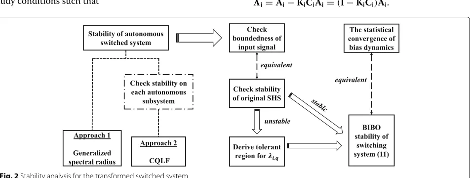
Among the existing research works, there are primarily two approaches to address the stability of the autonomous switched system in (11). One approach involves solving the generalized/joint spectral radius (JSR) of a bounded set of matrices [39]. As proved in [40], testing whether the JSR of a bounded set of matrices is less than or equal to 1 is computationally undecidable. While the exact compu-tation of JSR is Turing-undecidable in general, the approx-imation of JSR is an active area of research. The other approach is primarily built on the well-known Lyapunov theory. Specifically, it has been proved that the existence of a common quadratic Lyapunov function (CQLF) pro-vides a sufficient condition for the asymptotic stability of the switched system in (11) which also implies the JSR of the bounded set of matrices is less than 1. Therefore, without dwelling on the approaches that involve approx-imations of JSR, our main results are built on Lyapunov theory. The analysis procedure is summarized in Fig.2.

We use to denote the subsystem

corresponding to modeq. The autonomous switched sys-tem (11) switches between for all q. The following lemma is introduced in [41].

Lemma 1The switched system (11) is asymptotically stable under arbitrary switching signal if:

(i).ρ(Fq) <1,∀q∈Q;

(ii).∃P=P0, F_qPFq−P≺0.

Condition (i) in Lemma1implies asymptotic stability of every subsystem and condition (ii) is the existence of common Lyapunov quadratic function (CQLF). Also, it is worth pointing out that the stability for each subsystem does not imply asymptotic stability of the switched system [42]. The converse does not always hold either. As dis-cussed in [43], by choosing the switching signal carefully, the switched system can be made asymptotically stable even though the subsystem is not. In the following, we first study conditions such that

ρ(Fq) <1,∀q∈Q (12)

holds, i.e., each subsystem is asymptotically stable.

4.1 Stability of subsystem

By definition,Fq is composed of convex combination of

matrices as:

Fq= d

i=1

λi,qi

The task of checking spectral radius of summation of matrices is not trivial in general. If two matrices are com-mutable, i.e., AB = BA, then ρ(A+B) ≤ ρ(A) + ρ(B) [44]. If all the matrices are non-negative (element-wise), [45] proves that spectral radius is strictly convex. But all the mentioned results cannot be extended to general cases. Therefore, directly checking the spectral radius is not feasible. An alternative approach is built on Lyapunov theory which demonstrates the relationship between a quadratic Lyapunov function (QLF) and the spectral radius of system matrices.

Lemma 2The following statements are equivalent: (i) if there exists a positive definite matrixPsuch that F_qPFq−P≺0;

(ii)ρ(Fq) <1;

(iii) the subsystem is asymptotically stable.

We first illustrate a property related to the spectral radius ofiin the following lemma.

Lemma 3For a switched system defined in (1), if

(Ai,BiQB_i)is controllable and(Ci,Ai)is observable for all i∈Q, then∀i∈Q,ρ(i) <1.

ProofFrom the definition,

i=Ai−KiCiAi=(I−KiCi)Ai.

For any Kalman filter, the observer gain corresponding to modeiis defined asLi = AiMiC_iCiMiC_i+R−1. Here, Miis the steady error covariance related to steady Kalman gainKi. Given thatAi,BiQB_iis controllable and(Ci,Ai) is observable for alli∈Q, the closed-loop dynamicsAi− LiCiis stable. That is,

ρ(Ai−LiCi) <1. Rewrite it as:

Ai−LiCi=Ai−AiKiCi=Ai(I−KiCi).

From commutativity property of spectral radius, ρ(Ai−LiCi)=ρ(i) <1.

With the fact that all the matricesiare stable, we have the following theorem.

Lemma 4If there is only oneλi,q>0for each q∈Q, then the subsystem is asymptotically stable for all q∈Q.

ProofLetkqbe the index indicating the non-zeroλkq,q

for eachq∈Q; note thatkqalso takes value inQ. Based on

the property of random variabletdiscussed in Section3, λkq,q=1. Therefore, we have

Fq=kq,∀q.

From Lemma 3, it is straightforward to conclude that ρ(Fq)= ρ(kq) <1,∀q∈ Q. According to Lemma2, all

the subsystems are asymptotically stable.

Following the notation in proof of Lemma4, we usekq

to denote the index indicating the non-zeroλkq,qfor each

q ∈ Q. Note that kq is not necessarily equal to q. As

ρ(q) <1 for allq, even though the probability of mode

mismatch betweenqand modekqis 1 (i.e., the mode

mis-matches always happen), all the subsystems are still stable. The physical interpretation behind the result seems inconsistent. However, this result is only related to the sta-bility of the autonomous subsystem but not the complete switched system. In fact, if we take a close look at our sys-tem in (10), the choice ofλ_kq,q will have impact on the input matrixGq. We will discuss this result in Section4.3.

Lemma4gives a non-trivial condition such that the sta-bility of each subsystem is guaranteed. However, the condition that only oneλi,q > 0 is not generally realistic

since it eliminates the randomness associated with errors. The next theorem is built on the concept of CQLF and it is applicable for broader choices ofλi,q.

Theorem 2 If for all i ∈ Q, i share a common quadratic Lyapunov function. That is, if there exists a positive definite matrixP∈Rn×nsuch that

iPi−P≺0,∀i∈Q, (13)

then every subsystem ∀q ∈ Qis

asymptoti-cally stable for all choices ofλi,q.

Proof

iPi−P≺0⇐⇒(a) P−iPi0 (b) ⇐⇒

P i i P−1

0.

(a) is due to the fact thatPis positive definite and (b) is a result of Schur decomposition. According to Lemma2, in order to prove is asymptotically stable for allq, we need to find if there exists some positive definite matrix Pqfor eachqsuch thatPq−FqPqFq0.

SinceP−iPi0, therefore,P−λ2i,qiPi0 for 0≤ λi,q≤1. For allq∈Q, we have:

P λi,qi λi,qi P−1

0=⇒

d

i=1

P λi,qi λi,qi P−1

0

=⇒

⎡ ⎢ ⎢ ⎢ ⎣ P

d i=1λ

i,qi

d i=1λ

i,qi P−1 ⎤ ⎥ ⎥ ⎥

⎦0

=⇒

P Fq

F_q P−1

0=⇒P−FqPFq0.

By taking Pq = P, we proved that there exists positive

definite matrixPqfor eachq such thatPq−FqPqFq0.

Therefore, every subsystem ∀q ∈ Q is

asymptotically stable for all choices ofλi,q.

As presented in Lemma1, there are two conditions that can guarantee the stability of the autonomous switched system. Condition (i) is related to the stability of each sub-system and we have developed Lemma4and Theorem2 determineρ(Fq) < 1 for allq ∈Q. To complete the

sta-bility analysis for switched autonomous system in (11), we will study conditions such that constraint (ii) in Lemma1 is satisfied in the following subsection.

4.2 Stability of switched autonomous systems

Their approach is based on the stability of the matrix pen-cil constructed using the state matrices corresponding to the two modes. While the matrix pencil presents a dif-ferent perspective on the CQLF existence problem, it also lacks an analytical solution.

In this work, the switched system in (11) contains unknown variableλi,qin the subsystem matricesFq. Due

to the unknown values inFq and lack of algebraic

solu-tions, we cannot directly solve the LMI conditions nor derive constraints onλi,qsuch that the existence of CQLF

forFqis guaranteed. In the following, we propose to

estab-lish a relationship between the existence of CQLF fori andFqand then obtain conditions for stability of switched

system (11) regardless of the choice ofλi,q.

Theorem 3If there exists a CQLF fori,∀i ∈ Q, then there exists a CQLF for Fq,∀q ∈ Q. As a consequence, the switched system (11) is asymptotically stable under arbitrary switching signal.

ProofWe will use the similar approach as shown in the proof of Theorem2. If there exists a CQLF fori, we know that there exists a positive definite matrixP∈Rn×nsuch that

iPi−P≺0,∀i∈Q.

As a result of Theorem2, for allq∈Q, we have

d

i=1

P λi,qi λi,qi P−1

0=⇒

P Fq

FqP−1

0=⇒F_qPFq−P≺0.

Therefore, there exists a CQLF for Fq,∀q ∈ Q. From

Lemma1, the switched system (11) is asymptotically sta-ble under arbitrary switching signal.

The condition derived in Theorem3is only based on all the matricesiwhich can be determined given the sys-tem matrix. The LMI condition can be easily checked in practice via an LMI solver alleviating the lack of an ana-lytical solution. As illustrated in Fig.2, we have completed the discussion for the stability of autonomous switched system (11) thus far. In the following, we will consider sta-bility of the complete transformed switched system (10) including the input term.

4.3 Bounded-input bounded-output (BIBO) stability

For the transformed switched system in (10), we introduce the notion of BIBO stability that has been defined in [48].

Definition 2The system in (10) isBIBO stableif there exists a positive constantη such that for any essentially bounded input signalu, the continuous statex∗satisfies

sup

k≥0

x∗k≤ηsup k≥0

uk.

According to this definition, an input signal cannot be amplified by a factor greater than some finite con-stantηafter passing through the system if the system is BIBO stable. It has been proven that if the correspond-ing autonomous switched system (11) is asymptotically stable, then the input-output system (10) is BIBO stable provided the input matrix Gq is uniformly bounded in

time for allq[49]. This in fact is the case when the system switches between a finite family of matrices. In our trans-formed switched system, the input signaluk =xk, where

xk is the continuous state of original system (1).

There-fore, depending on the stability of (1), uk can be either

bounded or unbounded. Therefore, we should consider two different scenarios based on the boundedness ofukin

the following discussions.

Scenario 1: Original system in (1) is not asymptoti-cally stable

If the original system in (1) is unstable, then sup_k≥0uk = supk≥0xk = ∞. Since uk is an n

-dimensional vector, whenuk is unbounded, at least one

of the elements in the vector is unbounded. We refer to those elements as unstable components and these components are collected in the setI:

I =

i: sup

k≥0

u[i]_k = ∞

.

For this situation, if the columns ofGqcorresponding to

those unstable components ofuk are 0, then the

bound-edness of sup_j≥0,qGquj is guaranteed. The process of

finding the stable region for each probability of mode mismatch error is summarized in Algorithm 2:

Algorithm 2Find stable region ofλi,q

1: Analyze stability of the original SHS 2: Find unstable components→I 3: forall q∈Qdo

4: foralli∈Qdo 5: LetT=i−i,q

6: if∃j∈Is.t.jthcolumn ofTis not 0then 7: λi,q=0

8: else

9: 0≤λi,q≤1

10: end if

11: end for

12: Solve

i

λi,q=1 for all non-zeroλi,q

13: end for

Generally,λi,q=1 fori=qshould always be a solution

of Algorithm 2 because ofi = i,qfori = q.

Further-more, this condition along with the result of Lemma 4 indicate thatλi,q = 1 fori = q not only guarantees

system in (10). By definition, λi,q represents the

prob-ability that true mode is q while estimated mode is i. λi,q = 1 fori = qmeaning that there is no mode

mis-match error. Therefore, the convergence ofx∗k (i.e., the

bias generated from mode-based Kalman filter) is reason-able. Besides the trivial solution, Algorithm 2 also gives a less conservative result. For those unstable components in the original SHS, if the difference ofi−i,qat the

col-umn corresponding to the unstable components are all 0, the mode-based Kalman filter is still tolerant of the mode mismatch betweeniandq.

Scenario 2: Original system in (1) is asymptotically stable

If the original system in (1) is asymptotically stable, then the continuous statexk (i.e., uk in the transformed

switched system) is bounded. Since linear transformations of a vector is a bounded operator in Euclidean space, for a bounded vectoru,Guis bounded. For this situation, we are interested in minimizing the upper bound of x∗k.

From the definition of BIBO stability, we can write x∗k≤ηsup

equality in (a) holds if and only if each row ofGqis linearly

dependent ofukfor allq,k. In this framework, we seek to

address the following questions:

(1) Given the probability of mode mismatch isP, i.e.,

d

largest tolerant region for mode mismatch probabilityP that will guarantee thatBis achievable?

The following theorem is developed to answer the first question.

Theorem 4 Given the probability of mode mismatch

P =0and the original system in (1) is asymptotically sta-ble, the lowest upper bound ofx∗kthat can be achieved

ProofFrom the definition ofGq,

Gq=

function ofGq. Given the constraint on mode mismatch

probability and results of (15) and (16), we get the lowest upper bound ofx∗kthat can be reached is:

To assist in the analysis for the second question, we first define an auxiliary functionφ:Rd−1→Ras: q. The following lemma illustrates the convexity of this function.

Lemma 5φ(υυυ)is a convex function respect toυυυ.

Proof In order prove that φ(υυυ) is a convex function respect toυυυ, we want to show that for allυυυ,ννν∈Rd−1_{, and}

Thereforeφ(υυυ)is a convex function onυυυ.

Recall that the second question is to derive the largest tolerant region for mode mismatch probability P such that an upper boundB of x∗k is achievable. In other

words, we need to solve forλi,qsuch thatdi=1

i=qλi,q = P

x∗k≤ηmax

we will use triangle inequality to approximateφ(λλλ)and get a more conservative condition. Since

φ(λλλ)≤max

is a 1st degree polynomial inequality withd−1 variables, and this can provide a feasible region for eachλi,qon the d−1 dimensions space.

The discussion of BIBO stability completes the conver-gent analysis of bias dynamics in a mode-based Kalman filter. Both stable and unstable original SHS have been taken into consideration. For an unstable system, we can still stabilize the bias dynamics by specifically choosing the probabilityλi,q. For an asymptotically stable system,

we addressed two important questions regarding the min-imization of the upper bound for the bias.

5 Experimental results

In this section, we conduct two experiments to verify our main results in Section4. We first consider a second-order switched system with two discrete states. Then, we illus-trate the value of the theoretical results on a small scale smart grid set up.

5.1 Example 1: Switched system with two discrete states

Consider a switched system with two discrete statesQ=

{1, 2}. The continuous state is a two-dimensional vector. Define matricesA,B, andCas:

A1=

By solving the feasibility of two LMIs that defined in (13), the result shows that1and2share a CQLF. Based

on Theorem3, there exists a CQLF forF1andF2with any

choice ofλ1,1,λ1,2,λ2,1,λ2,2. Therefore, the switched

sys-tem composed with and is asymptotically stable under arbitrary switching signal.

The next step is to study the boundedness ofuk (i.e.,

xk of the original system). The boundedness of xk can

be checked by the existence of CQLF between A1 and

A2. With a similar LMI condition, it shows that the

orig-inal system is asymptotically stable. Therefore, the bias dynamics in the mode-based Kalman filter should be BIBO stable with upper bounds derived in (14).

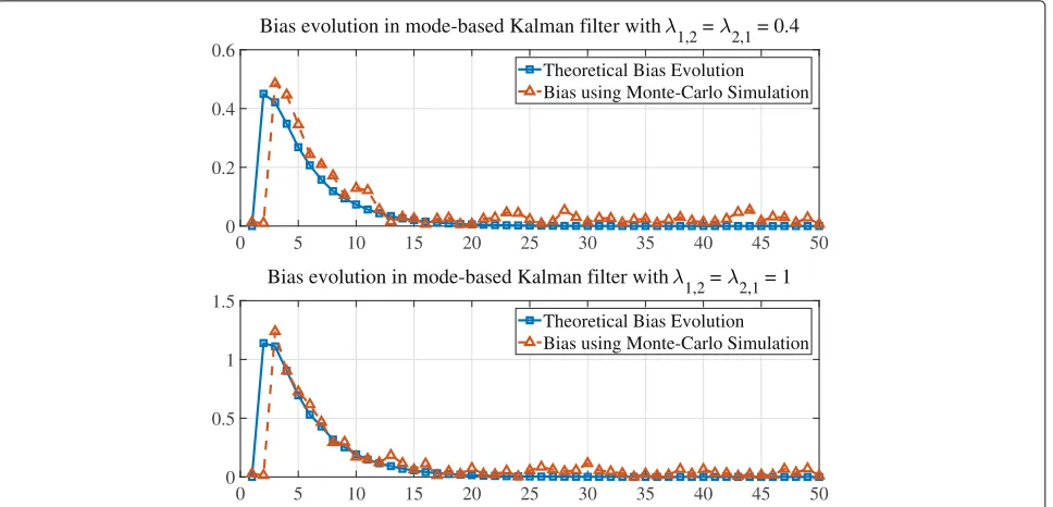
Figures 3 and4 are the experiment results overN = 5000 Monte-Carlo simulation for two different switching signals. For each switching signal, two different probabil-ities of mode-mismatch errorλ1,2andλ2,1were

consid-ered. In both Figs.3 and4, we plot the theoretical bias performance in line with squares. The theoretical bias is obtained via Eq. (9). The actual bias dynamics (difference ofE(xˆk)andE(xk)) from Monte-Carlo simulation is

0 5 10 15 20 25 30 35 40 45 50 0

0.2 0.4 0.6

Bias evolution in mode-based Kalman filter with

1,2 = 2,1 = 0.4

Theoretical Bias Evolution Bias using Monte-Carlo Simulation

0 5 10 15 20 25 30 35 40 45 50 0

0.5 1 1.5

Bias evolution in mode-based Kalman filter with

1,2 = 2,1 = 1

Theoretical Bias Evolution Bias using Monte-Carlo Simulation

Fig. 3Bias in mode-based Kalman filter using Monte-Carlo simulation and theoretical bias evolution for switching signal 1

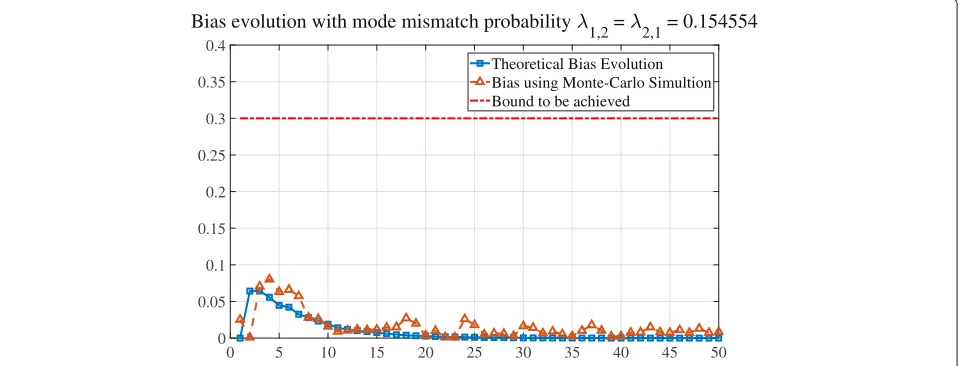
In Fig. 5, the line with squares shows the maximum value for norm of bias over Monte-Carlo simulation given that probability of mode mismatch isP. The dashed line is the upper bound calculated using Theorem4. In Fig.6, we seek to address question (2) proposed in the last section. That is, we want to achieve a certain upper boundB = 0.3 for the bias dynamics. By solving Eq. (18), the max-imum probability of mode mismatch is λ1,2 = λ2,1 =

0.154554. Figure6 shows the actual and theoretical bias evolution with mode mismatch error λ1,2 = λ2,1 =

0.154554. We can conclude that the target bound has been achieved.

0 5 10 15 20 25 30 35 40 45 50

0 0.05 0.1 0.15 0.2

Bias evolution in mode-based Kalman filter with _1,2 = _2,1 = 0.3

Theoretical Bias Evolution Bias using Monte-Carlo Simulation

0 5 10 15 20 25 30 35 40 45 50

0 0.1 0.2 0.3 0.4

Bias evolution in mode-based Kalman filter with _1,2 = _2,1 = 0.8

Theoretical Bias Evolution Bias using Monte-Carlo Simulation

Fig. 4Bias in mode-based Kalman filter using Monte-Carlo simulation and theoretical bias evolution for switching signal 2

5.2 Example 2: Smart grid

A classic example of a cyber-physical system that can be modeled in the SHS framework is a smart grid. We have defined the system model in Section 2.2. For this case study, the status of componentsL,GandDand the grid parameters are defined in Table1. Based on system set-tings,kG,α,σGandσDcompletely determine the system

matricesAqandBq. LetCq=Ifor all modes. Define the

noise aswk ∼N(0,Q)andvk∼N(0,R)withQ=2×I

and R = I. With this system setting, we get 1 =

0.9817, 2 = 0.8837, and3 = 0.8611. Therefore,

similar as (19), we haveρ(F1),ρ(F2), andρ(F3) < 1 for

all choices ofλi,t. The next step is to solve the LMI

condi-tions on1,2, and3and the results shows that1,2,

and3share a CQLF. Based on Theorem3, the switched

system composed with , , and is asymptotically

0 0.1 0.2 0.3 0.4 0.5 0.6 0.7 0.8 0.9 1

Probability of mode mismatch error (P)

0 0.5 1 1.5 2

2.5 Upper bound on norm of bias for different P

Max ||x*

k|| over [0,3000]

Upper Bound of ||x*_k||

0 5 10 15 20 25 30 35 40 45 50 0

0.05 0.1 0.15 0.2 0.25 0.3 0.35 0.4

Bias evolution with mode mismatch probability

1,2 = 2,1 = 0.154554

Theoretical Bias Evolution Bias using Monte-Carlo Simultion Bound to be achieved

Fig. 6To achieve an upper bound of biasB₌0.3, the bias evolution with probability of mode mismatch as_λ1,2=λ2,1=0.154554

stable under arbitrary switching signal. In order to check the boundedness of inputuk, we solve for the CQLF for

A1,A2, andA3. In this case, the result reveals that the

orig-inal SHS is not stable (falls into scenario 1 in Section4.3). Therefore, we are able to use Algorithm 2 to derive the stable region of each λi,q. In this system, the unstable

component is:I = {1}, i.e., only the first element is unsta-ble. Based on Algorithm 2, we need to calculateTi,qand

find out the corresponding elements on column 1 of each matrix. We get:

T1,2=

−0.3303 0

0 0.0385

,T1,3=

−0.3303 0

0 0.0375

,

T2,1=

0.1827 0

0 −0.0361

,T2,3=

0 0 0 −0.0088

,

T3,1=

0.1745 0

0 −0.0342

,T3,2=

0 0 0 0.0086

.

It can be observed that the first column inT2,3andT3,2

are 0. Therefore, the mode-based Kalman filter can be tol-erant on mode mismatch error between mode 2 and mode 3. The stable region for eachλis:

λ1,2=λ1,3=λ2,1=λ3,1=0

0≤λ2,3,λ3,2,λ1,1,λ2,2,λ3,3≤1.

Note that the condition that 3i=1λi,q = 1 should also

hold for every q. Figure 7 shows a Monte-Carlo simu-lation for two different λsettings. For Setting I, we use λ2,1 = λ3,1 = λ1,2 = λ1,3 = 0,λ3,2 = 0.4,λ2,3 = 0.7

Table 1Discrete status and continuous dynamics parameters

Status L G D q kG α σG σD

Failure mode 0 0 0 1 0.1 0.1 0.1 0.1

Grid connected 1 1 0 2 3 0.5 0.8 0.8

1 1 1 3 3 0.49 1.5 1

where all theλs are within the stable region. The simula-tion results for Setting I are shown in lines with squares and triangles with lefty-axis. Specifically, the line with squares is the theoretical bias derived using the bias evo-lution Eq. (10) while the line with triangles shows the bias in a mode-based Kalman filter via Monte-Carlo simula-tion. We can conclude that when all theλs are in stable region, the bias of the mode-based Kalman filter is con-vergent and bounded. For Setting II, we useλ2,1=λ3,1=

λ1,2 = 0.1,λ1,3 = 0,λ3,2 = 0.3,λ2,3 = 0.2 in whichλ2,1,

λ3,1, andλ1,2are outside the stable region. The solid line

and the dashed line with righty-axis present the results for theoretical bias and actual bias generated in a mode-based Kalman filter via Monte-Carlo simulation. Note that they-axis on the right is logx∗_ksince the actualx∗_k explodes rapidly. As this system does not have tolerance between mode 1,2 and mode 1,3, even a small probability of error (i.e., 0.1 in this case) will result in rapid explosion in the bias dynamics.

6 Conclusions and future work

0 5 10 15 20 25 30 35 40 45 50

Time Index 0

0.1 0.2 0.3 0.4 0.5

Norm(Bias)

-3 -2 -1 0 1 2 3

log

10

Norm(Bias)

Evolution of bias with two different settings

Theoretical bias for Setting I Actual bias for Setting I Theoretical bias for Setting II Actual bias for Setting II

Fig. 7Monte-Carlo simulation for the smart grid system with_λin stable region and unstable region

Abbreviations

BIBO: Bounded-input bounded output; CQLF: Common Lyapunov quadratic function; IMM: Interacting multiple model; LMI: Linear matrix inequality; MJLS: Markov jump linear system; MMAE: Multiple model adaptive estimation; MMSE: Minimum mean square error; MSE: Mean squared error; PV: Photovoltaics; QLF: Quadratic Lyapunov function; SHS: Stochastic hybrid system

Acknowledgements

The authors would like to thank the reviewers for providing valuable feedback on the manuscript.

Funding

This research was supported by the National Science Foundation through the award no. CNS-1544705.

Availability of data and materials

Data sharing is not applicable to this article as no datasets were generated or analyzed during the current study.

Authors’ contributions

Both authors contributed to the theoretical analysis and manuscript writing. Both authors read and approved the final manuscript.

Competing interests

The authors declare that they have no competing interests.

Publisher’s Note

Springer Nature remains neutral with regard to jurisdictional claims in published maps and institutional affiliations.

Received: 11 April 2018 Accepted: 4 November 2018

References

1. J. Hu, W.-C. Wu, S. Sastry,Modeling subtilin production in Bacillus subtilis using stochastic hybrid systems. (Springer, Berlin, 2004), pp. 417–431 2. A. Singh, J. P. Hespanha, Stochastic hybrid systems for studying

biochemical processes. Philos. Trans. R. Soc. Lond. A Math. Phys. Eng. Sci. 368(1930), 4995–5011 (2010).https://doi.org/10.1098/rsta.2010.0211 3. M. K. Ghosh, A. Arapostathis, S. I. Marcus, Optimal control of switching

diffusions with application to flexible manufacturing systems. SIAM J. Control. Optim.31(5), 1183–1204 (1993).https://doi.org/10.1137/0331056 4. J. P. Hespanha,Stochastic hybrid systems: application to communication

networks. (R. Alur, G. J. Pappas, eds.) (Springer, Berlin, 2004), pp. 387–401 5. W. Glover, J. Lygeros,A stochastic hybrid model for air traffic control

simulation. (Springer, Berlin, 2004), pp. 372–386

6. M. Prandini, J. Hu, inDecision and Control, 2008. CDC 2008. 47th IEEE Conference On. Application of reachability analysis for stochastic hybrid systems to aircraft conflict prediction, (2008), pp. 4036–4041.https://doi. org/10.1109/CDC.2008.4739248

7. M. Stˇrelec, K. Macek, A. Abate, in2012 3rd IEEE PES Innovative Smart Grid Technologies Europe (ISGT Europe). Modeling and simulation of a microgrid as a stochastic hybrid system, (2012), pp. 1–9.https://doi.org/10.1109/ ISGTEurope.2012.6465655

8. Y. Huang, M. Esmalifalak, Y. Cheng, H. Li, K. A. Campbell, Z. Han, Adaptive quickest estimation algorithm for smart grid network topology error. IEEE Syst. J.8(2), 430–440 (2014).https://doi.org/10.1109/JSYST.2013.2260678 9. G. Welch, G. Bishop,An introduction to the Kalman filter. Technical report,

(Chapel Hill, 1995)

10. H. J. Chizeck, Y. Ji, inDecision and Control, 1988., Proceedings of the 27th IEEE Conference On. Optimal quadratic control of jump linear systems with Gaussian noise in discrete-time, (1988), pp. 1989–19933.https://doi.org/ 10.1109/CDC.1988.194681

11. M. H. A. Davis, R. B. Vinter,Stochastic modelling and control. Monographs on statistics and applied probability. (Chapman and Hall, USA, 1985) 12. O. L. V. Costa, M. D. Fragoso, R. P. Marques,Discrete-time Markov jump

linear systems. Applied probability. (Springer, USA, 2005).https://books. google.com/books?id=4vyzaB6G3O0C

13. I. Matei, N. C. Martins, J. S. Baras, in2008 American Control Conference. Optimal state estimation for discrete-time markovian jump linear systems, in the presence of delayed mode observations, (2008), pp. 3560–3565.https://doi.org/10.1109/ACC.2008.4587045

14. I. Matei, J. S. Baras, Optimal state estimation for discrete-time Markovian jump linear systems, in the presence of delayed output observations. IEEE Trans. Autom. Control.56(9), 2235–2240 (2011).https://doi.org/10.1109/ TAC.2011.2160027

15. C. E. Seah, I. Hwang, Stochastic linear hybrid systems: modeling, estimation, and application in air traffic control. IEEE Trans. Control. Syst. Technol.17(3), 563–575 (2009).https://doi.org/10.1109/TCST.2008. 2001377

16. W. Liu, C. E. Seah, I. Hwang, inDecision and Control, 2009 Held Jointly with the 2009 28th Chinese Control Conference. CDC/CCC 2009. Proceedings of the 48th IEEE Conference On. Estimation algorithm for stochastic linear hybrid systems with quadratic guard conditions, (2009), pp. 3946–3951.https:// doi.org/10.1109/CDC.2009.5400909

17. W. Zhang, B. Natarajan, in2016 54th Annual Allerton Conference on Communication, Control, and Computing (Allerton). State estimation in stochastic hybrid systems with quadratic guard conditions, (2016), pp. 752–757.https://doi.org/10.1109/ALLERTON.2016.7852308 18. M. W. Hofbaur, B. C. Williams, inHybrid Systems: Computation and Control:

19. H. A. P. Blom, Y. Bar-Shalom, The interacting multiple model algorithm for systems with Markovian switching coefficients. IEEE Trans. Autom. Control.33(8), 780–783 (1988).https://doi.org/10.1109/9.1299 20. C. B. Chang, M. Athans, State estimation for discrete systems with

switching parameters. IEEE Trans. Aerosp. Electron. Syst.AES-14(3), 418–425 (1978).https://doi.org/10.1109/TAES.1978.308603 21. J. Tugnait, Adaptive estimation and identification for discrete systems

with Markov jump parameters. IEEE Trans. Autom. Control.27(5), 1054–1065 (1982).https://doi.org/10.1109/TAC.1982.1103061

22. B. Sinopoli, L. Schenato, M. Franceschetti, K. Poolla, M. I. Jordan, S. S. Sastry, Kalman filtering with intermittent observations. IEEE Trans. Autom. Control.49(9), 1453–1464 (2004).https://doi.org/10.1109/TAC.2004. 834121

23. X. Liu, A. Goldsmith, inDecision and Control, 2004. CDC. 43rd IEEE Conference On, vol. 4. Kalman filtering with partial observation losses, (2004), pp. 4180–41864.https://doi.org/10.1109/CDC.2004.1429408 24. E. Rohr, D. Marelli, M. Fu, in49th IEEE Conference on Decision and Control

(CDC). Statistical properties of the error covariance in a Kalman filter with random measurement losses, (2010), pp. 5881–5886.https://doi.org/10. 1109/CDC.2010.5717554

25. S. Deshmukh, B. Natarajan, A. Pahwa, State estimation over a lossy network in spatially distributed cyber-physical systems. IEEE Trans. Signal Process. 62(15), 3911–3923 (2014).https://doi.org/10.1109/TSP.2014.2330810 26. M. Moayedi, Y. C. Soh, Y. K. Foo, in2009 American Control Conference.

Optimal kalman filtering with random sensor delays, packet dropouts and missing measurements, (2009), pp. 3405–3410.https://doi.org/10.1109/ ACC.2009.5160216

27. B. Yan, H. Lev-Ari, A. M. Stankovic, Networked state estimation with delayed and irregularly-spaced time-stamped observations. IEEE Trans. Control Netw. Syst.PP(99), 1–1 (2017).https://doi.org/10.1109/TCNS. 2017.2653422

28. S. M. S. Alam, B. Natarajan, A. Pahwa, in2015 IEEE Global Communications Conference (GLOBECOM). Agent based optimally weighted kalman consensus filter over a lossy network (IEEE, USA, 2015), pp. 1–6 29. M. Nourian, A. S. Leong, S. Dey, D. E. Quevedo, An optimal transmission

strategy for Kalman filtering over packet dropping links with imperfect acknowledgements. IEEE Trans. Control. Netw. Syst.1(3), 259–271 (2014). https://doi.org/10.1109/TCNS.2014.2337975

30. S. Dey, A. Chiuso, L. Schenato, Remote estimation with noisy

measurements subject to packet loss and quantization noise. IEEE Trans. Control Netw. Syst.1(3), 204–217 (2014).https://doi.org/10.1109/TCNS. 2014.2337961

31. P. D. Hanlon, P. S. Maybeck, Characterization of Kalman filter residuals in the presence of mismodeling. IEEE Trans. Aerosp. Electron. Syst.36(1), 114–131 (2000).https://doi.org/10.1109/7.826316

32. I. Hwang, H. Balakrishnan, C. Tomlin, inDecision and Control, 2003. Proceedings. 42nd IEEE Conference On. Performance analysis of hybrid estimation algorithms, vol. 5, (2003), pp. 5353–53595.https://doi.org/10. 1109/CDC.2003.1272488

33. I. Hwang, H. Balakrishnan, C. Tomlin, inEuropean Control Conference (ECC), 2003. Observability criteria and estimator design for stochastic linear hybrid systems (IEEE, USA, 2003), pp. 3317–3322

34. C. E. Seah, I. Hwang, Algorithm for performance analysis of the IMM algorithm. IEEE Trans. Aerosp. Electron. Syst.47(2), 1114–1124 (2011). https://doi.org/10.1109/TAES.2011.5751246

35. I. Hwang, C. E. Seah, S. Lee, A study on stability of the interacting multiple model algorithm. IEEE Trans. Autom. Control.62(2), 901–906 (2017). https://doi.org/10.1109/TAC.2016.2558156

36. W. Zhang, B. Natarajan, in2018 Annual American Control Conference (ACC). Quantifying the bias dynamics in a mode-based Kalman filter for stochastic hybrid systems, (2018), pp. 5849–5856.https://doi.org/10. 23919/ACC.2018.8431697

37. D. Liberzon,Switching in Systems and Control. Systems & Control: Foundations & Applications, (Birkha user Boston, 2003)

38. R. Weron, B. Kozłowska, J. Nowicka-Zagrajek, Modeling electricity loads in California: a continuous-time approach. Physica A: Statistical Mechanics and its Applications.299(1), 344–350 (2001).https://doi.org/10.1016/ S0378-4371(01)00315-6. Application of Physics in Economic Modelling 39. R. Jungers,The joint spectral radius: theory and applications. Lecture Notes in

Control and Information Sciences. (Springer, Germany, 2009)

40. V. D. Blondel, J. N. Tsitsiklis, The boundedness of all products of a pair of matrices is undecidable. Syst. Control Lett.41(2), 135–140 (2000).https:// doi.org/10.1016/S0167-6911(00)00049-9

41. O. Mason, R. Shorten, On common quadratic Lyapunov functions for stable discrete-time LTI systems. IMA J. Appl. Math.69(3), 271 (2004). https://doi.org/10.1093/imamat/69.3.271

42. D. Liberzon, J. P. Hespanha, A. S. Morse, Stability of switched systems: a lie-algebraic condition. Syst. Control Lett.37(3), 117–122 (1999) 43. R. A. Decarlo, M. S. Branicky, S. Pettersson, B. Lennartson, Perspectives and

results on the stability and stabilizability of hybrid systems. Proc. IEEE. 88(7), 1069–1082 (2000).https://doi.org/10.1109/5.871309

44. F. Kittaneh, Spectral radius inequalities for Hilbert space operators. Proc. Am. Math. Soc.134(2), 385–390 (2006)

45. S. Friedland, Convex spectral functions. Linear Multilinear Alg.9(4), 299–316 (1981).https://doi.org/10.1080/03081088108817381

46. H. Lin, P. J. Antsaklis, Stability and stabilizability of switched linear systems: a survey of recent results. IEEE Trans. Autom. Control.54(2), 308–322 (2009).https://doi.org/10.1109/TAC.2008.2012009

47. R. Shorten, K. S. Narendra, O. Mason, A result on common quadratic Lyapunov functions. IEEE Trans. Autom. Control.48(1), 110–113 (2003) 48. R. Shorten, F. Wirth, O. Mason, K. Wulff, C. King, Stability criteria for

switched and hybrid systems. SIAM Rev.49(4), 545–592 (2007).https:// doi.org/10.1137/05063516X