Application to a Study of Chemical Order in
57Fe
3Al
Thesis by
Jiao Lin
In Partial Fulfillment of the Requirements for the Degree of
Doctor of Philosophy
California Institute of Technology Pasadena, California
2004
c
2004 Jiao Lin
Acknowledgements
I wish to express my gratitude to my advisor, Brent Fultz. His guidance,
encourage-ment, and advice have made this thesis possible.
I would like to acknowledge my predecessors in this project: Ushma Kriplani and
Martin Regehr. They led me to my first understanding of experimental and theoretical
issues involved.
I would like to thank my collegues in Keck lab: Ryan Monson, who is now taking
over the project, for his helpful discussions; Shu Miao for his help on getting TEM
works done; Channing Ahn for his assistance in routine lab issues and helpful
dis-cussions in TEM work; Carol Garland for her kind help on TEM works; Alan Yue,
Alex Papandrew, JaeDong Lee, Jason Graetz, Nathan Good, Olivier Delaire, Tabitha
Swan-Wood, and Tim Kelley, for sharing their thoughts and fun with me. I am also
grateful to other folks in Keck, for their kind help: Pam Albertson, Robin Hanan,
Elizabeth Welsh, etc.
I would like to thank Fiona Harrison for allowing us to use their CZT/CT
detec-tor technology, and to acknowledge her group members including Hubert Chen, Jill
Burnham, Rick Cook, ..., for their kind instructions and discussions about CZT/CT
detectors.
I am indebted to some students of Materials Science, 1999: Jian Wu, Lan Yang,
Qingsong Zhang and Tao Feng. They filled my stay in Caltech with fun and collision
of thoughts.
I am very grateful to my parents, Manqing Hu and Yingji Lin, and my younger
brother, Rong Lin. Their unconditional support are always there.
M¨
ossbauer Diffractometry: Principles, Practice, and an Application to a
Study of Chemical Order in
57Fe3
Al
by
Jiao Lin
In Partial Fulfillment of the
Requirements for the Degree of
Doctor of Philosophy
Abstract
For the first time, M¨ossbauer powder diffractometry went beyond the proof-of-principal
stage and was used to study unknown periodicities of defect-related chemical
envi-ronments of Fe atoms in a partially-ordered
57Fe3Al polycrystalline sample.
M¨ossbauer powder diffractometry is based on two phenomena, the M¨ossbauer
ef-fect and the Bragg diffraction. The M¨ossbauer efef-fect is sensitive to short-range
or-der whereas diffractometry is sensitive to long-range oror-der. Together, they enable
M¨ossbauer powder diffractometry to provide information on long-range periodicities
of target atoms having specific short-range order.
Both experimental and theoretical efforts are necessary for this novel technique
to become practial. In this research, hardware and software for M¨ossbauer powder
diffractometry were improved. A kinematical diffraction theory for M¨ossbauer powder
diffractometry incorporating effects of interference between electronic and nuclear
resonant scattering was developed. The applicability of the theory was verified by
computer calculations that accounted for dynamical diffraction effects. A thorough
analysis of polarization effects, including a polycrystalline average of polarization
factors, was done systematically using spherical harmonic expansions.
Multiple diffraction patterns were measured at Doppler velocities across all
nu-clear resonances of
57Fe
Contents
1 Introduction 1
1.1 An Intuitive Description of M¨ossbauer Powder Diffractometry . . . 1
1.2 M¨ossbauer Powder Diffractometry . . . 4
1.3 M¨ossbauer Diffraction Study of Fe3Al . . . 6
2 M¨ossbauer Effect 11 2.1 Recoilless Fraction . . . 12
2.2 Nuclear Resonance . . . 14
2.2.1 Isomer Shift . . . 15
2.2.2 Magnetic Dipole Hyperfine Interactions . . . 16
2.2.3 Electric Quadrupole Hyperfine Interactions . . . 17
2.3 M¨ossbauer Spectrum of Fe . . . 18
2.4 M¨ossbauer Spectrum of Fe3Al . . . 19
2.4.1 M¨ossbauer Spectrum and HMF Distribution . . . 19
2.4.2 Magnetic Polarization Model . . . 21
3 Quantum Theory of M¨ossbauer Absorption and Scattering 25 3.1 Interaction of a Photon and a Nucleus . . . 26
3.1.1 Transition Probability . . . 26
3.1.2 Interaction Matrix Element of Magnetic Transition . . . 29
3.1.3 Scattering . . . 31
3.1.4 Nuclear Absorption Cross Section . . . 41
3.2 Scattering Property of a Single M¨ossbauer Atom . . . 42
4 Kinematical Theory of M¨ossbauer Diffraction 45
4.1 Scattering Property of A M¨ossbauer Atom in a Thin Single-Crystal Sample . . . 45
4.2 Effects of Hyperfine Magnetic Field Distribution on Scattering Amplitudes of 57Fe Atoms . . . 48
4.2.1 Example 1: Distribution of Magnitudes of HMF . . . 49
4.2.2 Example 2: Orientational Distribution of HMF . . . 49
4.2.3 Possible Application for Studying Invar . . . 51
4.2.4 Summary . . . 52
4.3 Diffraction Intensity of a Polycrystalline Sample: Effects of Orientational Distribution of Hyperfine Magnetic Fields among Crystallites . . . 52
4.3.1 Scattering Cross Section . . . 53
4.3.2 Absorption Cross Section . . . 55
4.3.3 Samples with More Than One Atom in a Unit Cell . . . 56
4.4 Diffraction Intensity from a Polycrystalline Sample . . . 57
4.5 Application to a57Fe Polycrystalline Sample . . . . 57
4.6 Dynamical Theory of M¨ossbauer Diffraction . . . 61
4.6.1 Scattered Wave from a Thin Layer of Crystal . . . 62
4.6.2 Propagation of Waves . . . 65
4.6.3 Enhancement of Coherent Scattering Width . . . 68
4.7 Test for the Applicability of Kinematical Theory . . . 70
5 Instrumentation and Data Analysis Procedure 73 5.1 Diffractometer . . . 73
5.1.1 Detector . . . 75
5.1.2 Custom Circuits . . . 75
5.1.3 Data Collection . . . 81
5.2 General Data Reduction Procedure . . . 81
5.2.1 GCSAXI . . . 83
5.2.2 MDS . . . 88
5.2.3 MEF . . . 89
6 Chemical Periodicities in Fe3Al 91 6.1 First-Nearest-Neighbor Environments for B2 and D03 Chemical Order . . . 91
6.3 Diffraction Patterns and Determination of Long-Range Order . . . 94
6.3.1 Chemical Environment Selective M¨ossbauer Diffraction Patterns . . . 94
6.3.2 Energy Spectra of M¨ossbauer Diffraction Patterns . . . 97
6.3.3 Intensities of bcc Fundamental Diffractions . . . 98
6.3.4 Intensities of Superlattice Diffractions . . . 101
6.3.5 Long-Range Order . . . 104
6.3.6 Distribution of Chemical Environments on Four fcc Sublattices . . . 107
6.4 Is Kinematical Diffraction Theory Good Enough? . . . 107
6.5 B2 LRO of Fe Atoms with (3) Al 1nn . . . 110
6.5.1 Environment-Sensitive Diffraction Intensities from Monte-Carlo Simulations . 110 6.5.2 Homogeneous Disorder . . . 112
6.5.3 Effects of Antiphase Boundaries . . . 115
6.6 Conclusions . . . 119
7 Ongoing and Future Work 121 7.1 CdTe Detector . . . 121
7.1.1 CdTe/CdZnTe Detector . . . 123
7.1.2 Construction of a CdTe Detector . . . 124
7.1.3 Low-Noise Electronics . . . 124
7.1.4 Digital Signal Processing . . . 127
7.2 Future Development and Research . . . 128
A Quantum Description of Recoilless Fraction 131 B Average Polarization Factors 135 B.1 Contribution from Nuclear Resonant Scattering . . . 136
B.1.1 Spherical distribution of HMF . . . 139
B.1.2 The Case of Nearly Planar Distribution of HMFs . . . 140
B.2 Contribution from Rayleigh Scattering . . . 142
B.3 Contribution from Interference . . . 142
B.3.1 Spherical Distribution of HMF . . . 144
B.3.2 Nearly Planar Distribution of HMF . . . 144
B.4 Basic Formulas for the Representations of Rotation Group . . . 144
C Details about Data Reduction 147
C.1 Format of a “mds.in” File . . . 147
List of Figures
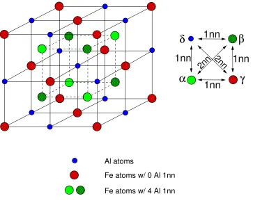
1.1 Fe3Al with the perfect D03 structure. This structure is a superposition of 4 fcc
sublattices,α,β, γandδ. Only the δ-sublattice is occupied by Al atoms while other
three sublattices are occupied by Fe atoms. . . 2
1.2 Fe3Al with the D03 structure in various resonance conditions: (a) off-resonance, (b) Fe atoms with (0) Al 1nn on resonance, (c) Fe atoms with (4) Al 1nn on resonance. The size of the balls indicates their cross section for incident photons. . . 3
1.3 Hyperfine magnetic field distribution calculated for a Fe3Al sample with the perfect D03 structure. . . 7
1.4 Hyperfine magnetic field distribution of a Fe3Al sample with a partial D03 order. . . 7
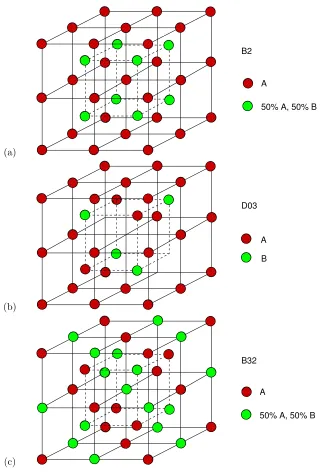
1.5 B2, D03 and B32 structure . . . 9
2.1 A M¨ossbauer spectrometer. . . 11
2.2 Recoil of a free nucleus hit by a photon . . . 12
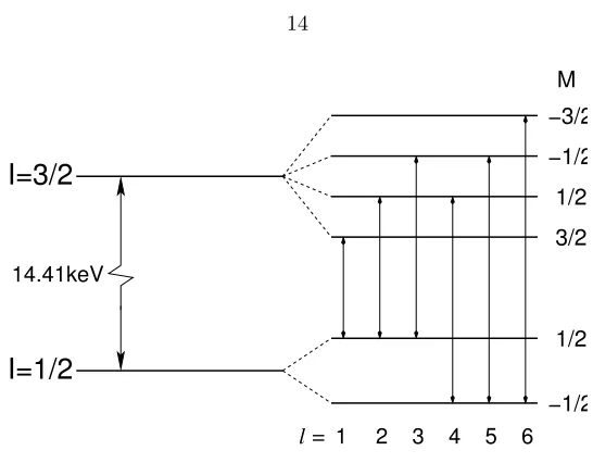
2.3 Transitions between ground state and 1st excited state of an 57Fe nucleus. . . . 14
2.4 A nucleus. It is assumed to have a uniform and spheric charge distribution. The nuclear radius isR. . . 15
2.5 A typical M¨ossbauer spectrum of natural Fe. . . 18
2.6 CEMS spectrum (thick, solid line) of a partially-ordered Fe3Al sample, and its de-composition into components of various chemical environments (Fe atoms with (0) Al 1nn : thin, solid line; (2) Al 1nn : dotted line; (3) Al 1nn : dashed line; (4) Al 1nn : dash-dot-dot-dot line) . . . 20
3.2 Feynman diagram of a second-order S-matrix. Time flows forward in the upwards
direction. A nucleus of state|nicombines with a photon|ωjmiand forms a nucleus
of state|li; it then de-excites to state|n0iby emitting a photon|ω0j0m0i. . . . 31
3.3 An example of high-order S-matrix representing scattering process. . . 35
3.4 A diagram with an ignorable correction to nuclear ground-state energy. . . 35
3.5 Polarization factor in M1 radiation. Each point on the surface represents a propaga-tion direcpropaga-tion of the photon,n. The distance from the point to the origin represents the amplitude of polarization factor. The change in color indicates the change in the phase of the polarization factor. . . 42
4.1 Scattering geometry. The indexesiandf indicate the incident and outgoing photons, respectively. Scattering is assumed to happen in the xy plane. The incident wave propagates in they direction. The polarization of index 1 is always parallel to thez direction, while that of index 2 is always perpendicular to thezdirection. . . 46
4.2 Scattering from a polycrystalline sample . . . 56
4.3 Orientational HMF distribution: isotropic and anisotropic . . . 58
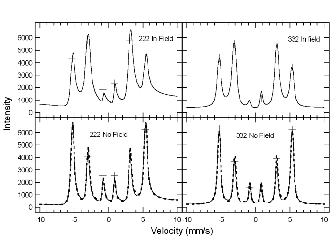
4.4 Calculated intensities for (222) and (332) M¨ossbauer diffractions from bcc57Fe. Crosses: experimental data. Solid lines: calculated from the isotropic model of HMF orienta-tions. Dashed lines: calculated from the anisotropic model. . . 59
4.5 Propagation of transmission and reflection waves. . . 66
5.1 Schematic of the M¨ossbauer powder diffractometer. . . 74
5.2 Operation of veto generator for Doppler drive running in constant velocity mode. Detector signals are collected only when the Doppler drive is at the desired velocity. At times when the Doppler drive is in regions of blue shadow, the detector is disabled by the veto generator. . . 75
5.3 Schematic design of the veto generator. . . 76
5.4 Logic design of the veto generator. . . 77
5.5 MCA counter in the veto generator. . . 78
5.6 Velocity controller schematic design. . . 79
5.7 Schematic design of the velocity read-back circuit. . . 79
5.8 Logic design of the velocity read-back circuit. . . 80
5.10 A typical SAXI image. Red curves show pixels of 2θ= 40, 50, 60, 70 and 80 degree. Some diffraction peaks are visible as bright stripes. . . 82
5.11 Geometry for determining the scattering angle, 2θ, of a detector pixel. . . 84 5.12 Data re-binning . . . 86
6.1 Distribution of Fe chemical environments for perfect A2, B2, D03, and B32 orders.
(A reproduction of Fig. 1.3 of Ref. [25]) . . . 92
6.2 Fe atoms with (3) Al 1nn as a result of one antisite defect. An antisite defect (purple)
is now in aδ-site. All iron atoms in its 1nn shell (green) now have 3 Al 1nn. . . 93 6.3 Four M¨ossbauer diffraction patterns from Fe3Al. Variations in detector sensitivity are
responsible for much of the background variations. . . 95
6.4 Difference of the M¨ossbauer diffraction patterns of figure 6.3 for (0), (4) and (3)
environments and off-resonance diffraction pattern. . . 96
6.5 M¨ossbauer diffraction patterns from57Fe
3Al, taken at 89 velocities arranged vertically.
Data were normalized by incident flux, and background was subtracted. . . 97
6.6 Full energy spectra of (211), (222) and (321) diffraction intensities from Fe3Al,
in-cluding kinematical theory calculations and experimental data. . . 99
6.7 Hyperfine magnetic field distribution obtained from energy spectra of (211), (222)
and (321) diffraction intensities of figure 6.6 compared to HMF distribution obtained
by CEMS. . . 100
6.8 Full energy spectra of (300) and (5 2 3 2 3
2) diffraction intensities from Fe3Al, including
kinematical theory calculations and experimental data. . . 103
6.9 Sensitivity of simulated energy spectra of (300) diffraction peak to variations of LRO
parameterηsc for (a) Fe atoms with (0) Al 1nn, (b) Fe atoms with (4) Al 1nn, and (c) Fe atoms with (3) Al 1nn. The thick lines are the best fit to experimental data
withη(0)sc =−0.98,ηsc(4)= 1.0 andη(3)sc = 0.59. Some lines are invisible due to overlap
with curves of the best fit: the thin line withη(0)sc =−1.0 in (a), and the dotted line
withη(4)sc = 1.0 in (b). . . 105
6.10 Sensitivity of simulated energy spectra of (5 2 3 2 3
2) diffraction peak to variations of LRO
parametersηfcc: (a) Im[ηfcc(0)], (b) Re[η
6.11 Energy spectra of M¨ossbauer diffraction peak (211) of Fe3Al calculated by the
6.12 Values ofχ2for the best fit to experimental spectra by the polycrystalline adaptation
of CONUSS, plotted against crystal thickness parameterζ. . . 109 6.13 Short-range order with random antisite defects, obtained from simulations of
homo-geneous disorder. The axisp(n) is the fraction of 57Fe atoms having the number n
Al atoms in their 1nn shell. Labels denote numbers, (n), of Al 1nn atoms about57Fe
atoms. . . 113
6.14 Long-range order with random antisite defects, obtained from simulations of
homo-geneous disorder. The LRO parameter,ηsc, was obtained from Eq. 6.9 . . . 113
6.15 Development of B2 LRO of the different Al neighborhoods of 57Fe, calculated by
Monte–Carlo simulation. Labels denote numbers, (n), of Al 1nn atoms about 57Fe
atoms. . . 115
6.16 Geometry of a B2-type APB on a (100) plane. The Fe atoms are represented by
bigger spheres and Al atoms are smaller. (a) A structure without APB. The Fe atom
at the center has 4 Al and 4 Fe 1nns. (b) A B2-type APB is inserted between the
central Fe atom and the 4 atoms on the left. . . 116
6.17 B2 type APBs on the (100) and (110) planes. Small, white balls are Al atoms. Big
atoms are all Fe atoms, in which color indicates number of Al 1nn, black:0, green:4,
white:2, blue:3, purple:1. It is clear that the B2-APB on the (100) plane consists of
Fe atoms with (2) Al 1nn; the B2-APB on the (110) plane consists of Fe atoms with
(3) and (1) Al 1nn. . . 116
6.18 TEM images of B2-type APBs in ordered Fe3Al: (a) bright-field image, (b) axial
dark-field image using a (100) superlattice diffraction, (c) axial dark-field image using
a (200) diffraction. . . 117
6.19 Diffraction patterns showing the conditions used for the bright-field and dark-field
images of Fig. 6.18. (a) (100) zone axis used, (b) actual tilt used for imaging. . . . 119
7.1 A schematic of a CdZnTe detector system. . . 123
7.2 A MISC board and a motherboard with one CdTe detector. . . 125
7.3 A schematic of the low-noise readout electronics for CdTe/CdZnTe detectors
devel-oped by Harrison’s group. . . 126
7.4 Energy spectrum of a 241Am source measured by a CdTe detector with all pixels
summed together. Only single-pixel events are included. . . 129
List of Tables
2.1 First-nearest-neighbor chemical environments in partially-ordered Fe3Al. . . 21
3.1 Facts about 6 transitions . . . 42
3.2 Comparison of diffraction techniques . . . 44
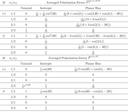
4.1 Polarization factors, P2 and P, for M¨ossbauer scattering averaged over the three
HMF distributions. The photon angular momentum in thezdirection is M, and the photon polarization indexes areni and nf. The diffraction angle is denoted by 2θ, and anglesβi andβf are defined in Fig. 4.2. . . 60
6.1 Parameters needed for all MDS and MEF calculations. . . 98
6.2 First-nearest-neighbors chemical environments in partially-ordered Fe3Al. . . 98
6.3 Phase factors for the four fcc sublattices in the D03 structure for (100)-type and
(121212)-type diffractions. . . 101 6.4 LRO parameters for prominent chemical environments of Fe and Al. . . 102
6.5 Concentration of chemical environments on the four fcc sublattices (experimental) . 107
6.6 Relative superlattice diffraction intensities of chemical environments in Monte-Carlo
simulated Fe3Al. . . 110
6.7 Superlattice diffraction intensities of chemical environments in Monte-Carlo simulated
Fe3Al. . . 111
6.8 Concentration of chemical environments in αand β fcc sublattices in case of homo-geneous antisite defect concentrationx. . . 114
7.1 Comparison of detectors. The CdTe detector system is assumed to be composed of 8
detectors as described in Table 7.2. The distance between the sample and the Bruker
detector is assumed to be 10 cm; for the CdTe detector it is assumed to be 12 cm.
7.2 Technical details about the CdTe detector . . . 122
Chapter 1
Introduction
1.1
An Intuitive Description of M¨
ossbauer Powder
Diffrac-tometry
M¨ossbauer powder diffraction is a novel technique combining the capability of M¨ossbauer
spectrom-etry to distinguish the chemical environments (short-range order) around specific target atoms1and
the capability of diffractometry to measure the long-range order. It enables studies of long-range
order of atoms with specific short-range order.
For example, look at the structure of an Fe3Al sample with perfect D03 structure in Fig. 1.1.
For iron atoms, two chemical environments exist. Fe atoms on theγ-sublattice (red) have no Al first nearest neighbors (1nn). Fe atoms with 4 Al and 4 Fe 1nn (green) occupy two face centered cubic
(fcc) sublattices,αandβ, and form a simple cubic (sc) long-range order. Theδ-sublattice is occupied by Al atoms. As is well known, M¨ossbauer resonance energies are very sensitive to the chemical
environments of the target atoms. Because the resonance energy of a 57Fe nuclei depends on its chemical environment, the absorption and scattering cross section of this iron atom are also strongly
dependent on its chemical environments. We can tune the energy of incident γ-ray photons to a specific chemical environment and then the atoms with this chemical environment will contribute
strongly to the diffraction pattern. For a more visual presentation, please take a look at Fig. 1.2.
Here, Al atoms are small, blue balls while Fe atoms are red, big balls. The size of an atom is used to
represent its scattering cross section; the bigger the atom, the stronger its scattering. Three different
resonance conditions are presented in this figure. In Fig. 1.2a, the incidentγ-ray is not on resonance for any atom, so the scattering cross section of Fe atoms are all the same, and 3 times larger than
Figure 1.1: Fe3Al with the perfect D03 structure. This structure is a superposition of 4 fcc
(a)
(b)
(c)
Figure 1.2: Fe3Al with the D03structure in various resonance conditions: (a) off-resonance, (b) Fe
atoms with (0) Al 1nn on resonance, (c) Fe atoms with (4) Al 1nn on resonance. The size of the
that of Al atoms2. This is in essence an X-ray diffraction experiment. In Fig. 1.2b, we tune theγ-ray
to be on resonance for iron atoms with zero Al 1nn, and they are now very strong scatterers. In Fig.
1.2c, iron atoms with 4 Al and 4 Fe 1nn are on resonance and will make the largest contribution
to scattered waves. Notice the approximate fcc structure in Fig. 1.2b and the sc structure in Fig.
1.2c, which give different diffraction patterns. As a result, diffraction patterns for these three cases
should show differences in intensities of superlattice diffraction orders. It is now very clear that with
M¨ossbauer diffraction, we can “see” the structure of specific chemical environments by tuning the
γ-ray energy.
The idea here sounds simple and powerful, but its realization requires both experimental and
theoretical developments. In the next Section, a review of these developments is presented.
1.2
M¨
ossbauer Powder Diffractometry
In X-ray diffraction, photons are scattered coherently by electrons. The scattered wave amplitude,
ψ, as a function of scattering vector,k, on a detector far from the scattering center, is proportional to the Fourier transform of scattering amplitude as a function ofrinside the crystal. Long-range order
(LRO) in the crystal will show itself as peaks in the diffraction pattern. The diffracted intensities can
reveal much information about the structure of the crystal under investigation. M¨ossbauer diffraction
involves coherent elastic scattering ofγ-ray photons by not only electrons but more importantly by nuclei in a sample containing at least one atomic species capable of nuclear resonant absorption
and re-emission. By tuning the energy of the incident γ-ray, a specific chemical environment of the M¨ossbauer nucleus can be emphasized, as shown in the previous Section, and its LRO can be
measured. Despite its promise as another powerful diffraction technique besides X-ray diffractometry,
transmission electron microscopy (TEM) and neutron diffractometry3, M¨ossbauer diffraction based
on kinematical theory [43, 7] was possible only very recently [61, 57, 35, 37], due to low count rates.
The coherence of M¨ossbauer scattering was first shown in the early 1960s by Black and Moon[10],
and the first M¨ossbauer diffraction measurements were performed a few years later[9]. However,
until very recently, most research on M¨ossbauer diffraction utilized perfect single crystals [9, 53, 62,
52]. Even today there is active development of M¨ossbauer dynamical diffraction using synchrotron
radiation (SR) sources (see, e.g., Ref. [47, 26, 59, 45]), which take advantage of the brightness of SR
for single crystal work. Unfortunately, multiple scattering is so strong for perfect single crystals that
2In this case, the only contribution comes from the electronic scattering, of which the atom scattering factor is approximately proportional to the number of electrons in the atom. Thus, σFe
dynamical diffraction theory [33, 28, 29, 32, 30] must be used to interpret the data. This makes it
impractical to invert single-crystal diffraction patterns to obtain quantitative information on atomic
structure.
Kinematical diffraction theory could be applicable for polycrystalline samples with small-enough
crystallites4. Polycrystalline diffraction experiments are more difficult than for oriented single
crys-tals, however, due to the low flux. The past decade has seen improvements in both instrumentation
and theory for M¨ossbauer powder diffractometry in the kinematical limit [61, 58, 57, 21, 35, 39, 38,
37]. Tegze and Faigel have built a M¨ossbauer powder diffractometer capable of gathering
diffrac-tion patterns from a cylindrical sample and they have obtained energy spectra from an enriched
ferromagnetic57Fe sample. The following developments were mostly made in the Fultz group at
Caltech.
Prior Experiment Stephens and Fultz [57] built the first powder diffractometer using an INEL
detector system. With this “first-generation” M¨ossbauer powder diffractometer, they performed a
“proof-of-principle” experiment, showing for the first time that in a 57Fe
3Al sample the diffraction
patterns of 57Fe atoms with 0 and 4 Al 1nn could be obtained by tuning the energy of the γ-ray
photons to resonance energies of these two chemical environments, respectively. Kriplani, Regehr
and Fultz adopted a Xe-filled, Bruker X-1000 detector in the “second-generation” M¨ossbauer powder
diffractometer. This area detector has better efficiency to 14.4 keV photons and better capability
for detecting photons off the scattering-plane, so the measured diffraction intensities were stronger.
Furthermore, this detector is relatively insensitive to high-energy photons, which contribute to
back-ground noise. This diffractometer was highly-automated in that the goniometer, the drive system,
and the detector system could be controlled by one computer program written in Visual Basicr. With the improved flux of this “second-generation” diffractometer, they were able to measure
co-herent and incoco-herent diffracted intensities at various resonance energies from a polycrystalline Fe57
sample. The effect of a magnetic field applied perpendicular to the scattering plane was also studied.
Prior Theory In his thesis, Stephens presented formalisms of kinematical diffraction theory
based on Patterson functions. Diffraction intensities were calculated using a multislice approach.
Kriplani[34] adopted Bara’s formalisms[5] to replace the multislice method and developed
system-atically a model for M¨ossbauer diffractive and incoherent scattering processes without considering
Rayleigh scattering from electrons. Her formalisms also incorporate the polarizing effects of a
netized sample.
Present Developments In this thesis, I
1. improved the diffractometer developed by Kriplani et al. and used it to measure for the first
time a full energy spectrum of complete M¨ossbauer diffraction patterns from a57Fe
3Al sample;
2. gave a kinematical diffraction theory taking into account both electrionic and nuclear resonant
scattering, and improved our understanding of the polarization factor and worked out the
averaged polarization factors involved in M¨ossbauer diffraction by using spherical-harmonic
expansions;
3. gave a more intuitive account for the M¨ossbauer scattering processes on the basis of
quan-tum electrodynamics and a simple account for the speed-up effect in dynamical M¨ossbauer
diffraction;
4. developed simulation programs for calculating diffraction intensities based on kinematical
diffraction theory;
5. verified the kinematical diffraction model by carry out simulations using dynamical diffraction
theory;
6. using these theoretical understanding and calculational tools, carried out fitting procedures to
find out optimal experimental parameters (long-range order parameters for various chemical
environments) in a partially-ordered57Fe 3Al;
7. interpreted these fitting results on the long-range order parameters of defect chemical
environ-ments, using Monte-Carlo simulations of kinetics of disorder-order transformation in Fe3Al,
simulations of homogeneous disorder, and transmission electron microscopy (TEM) studies of
anti-phase domains;
8. began the development of a “third generation” M¨ossbauer diffractometer using CdTe detectors.
The next Section provides more details for the motivation for studying Fe3Al.
1.3
M¨
ossbauer Diffraction Study of Fe
3Al
As shown in Section 1.1, Fe3Al with the perfect D03structure has two distinct chemical environments
25x10
-320
15
10
5
0
Probability
350
300
250
200
150
100
50
0
Hyperfine Magnetic Field (kG)
5 4 3 2 10
Figure 1.3: Hyperfine magnetic field distribution calculated for a Fe3Al sample with the perfect D03
structure.
15x10
-310
5
0
Probability
350
300
250
200
150
100
50
0
Hyperfine Magnetic Field (kG)
5 4 3 2 10
chemical environments show themselves as two distinct peaks in the HMF distribution (see Fig. 1.3).
This means we can really “turn on and off” the scattering power of Fe atoms of special chemical
environments by tuning the Doppler velocity ofγ-ray source, as explained in Section 1.1, so Fe3Al is
well-suited for study using M¨ossbauer diffraction. A first experiment would be to tune the photon
energy to be on resonance for Fe atoms of these two chemical environments and measure diffraction
patterns that should show different superlattice peaks. This has already been done by Stephens and
Fultz [57, 21, 56].
A second experiment could be suggested by Fig. 1.4, the HMF distribution of a real Fe3Al
sample. Notice that this sample shows chemical environments other than the two major chemical
environments of the perfect D03structure. The additional chemical environments are related to local
defects, but their spatial distributions are unknown. By tuning the photon energy to those chemical
environments we might be able to obtain information about the spatial periodicities of57Fe atoms in
these defects environments. A study of the evolution of these defects and their spatial distribution
along the path of disorder−→order transition could shed light on the kinetics of this transition in Fe3Al. As a first step, in this thesis research we have measured the M¨ossbauer diffraction intensities
at Doppler energies through the full M¨ossbauer spectrum of this57Fe
3Al sample (which was used in
the previous “proof-of-principle” experiment done by Stephens and Fultz[56]). These spectra can be
used to determine the long-range order of the defect-related Fe atoms. This is a natural development
of M¨ossbauer powder diffractometry: from a proof-of-principle experiment to exploration of unknown
properties of materials. In the course of this work, data analysis programs based on kinematical
diffraction theories including polarization effects were developed.
Order in Fe3Al At high temperatures, Fe3Al has the bcc structure, and develops sc order with
the B2 structure at temperatures below 800◦C. Below 550◦C the equilibrium structure is the D0
3
structure, where Al atoms occupy one of four fcc sublattices of the D03 structure (we denote this
Al-rich sublattice asδas show in Fig. 1.1). After Fe3Al is quenched rapidly, subsequent annealing at
low temperatures shows a number of peculiarities, such as the formation of the B32 structure, which
may be a kinetic transient [3, 24, 4], or perhaps driven by magnetic interactions in sub-stoichiometric
zones [6]. These ordered structure are shown in Fig. 1.5. In alloys with partial order, it is possible to
determine sublattice occupancies by the intensities of superlattice diffractions of x-rays or neutrons,
although occupancies become difficult to quantify when the state of order is high and the effects on
intensity are small. In many cases including non-equilibrium alloys with small grain sizes, M¨ossbauer
(a)
Fe atoms with different numbers of Al first-nearest neighbors5[54, 18, 19]. These defect environments
may have spatial periodicities of the D03structure, although the problem may not be simple owing
to expected statistical non-uniformities of composition or if the defect environments interact.
In this thesis research we made the first direct measurements of spatial periodicities of defect
environments in a material. Improved instrumentation for the present experiment made it possible
to go beyond measurements at resonance peaks of57Fe atoms in the known chemical environments
of the perfect D03structure. M¨ossbauer diffraction patterns were measured over the full M¨ossbauer
energy spectrum of the alloy, making it possible to quantify the unknown spatial periodicity of57Fe
atoms with (3) Al 1nn atoms. It is found that the Fe atoms in this defect environment have some
sc periodicity. The data were further analyzed to obtain the occupancies of the four sublattices of
the D03 structure, with no assumptions that would select B2 over B32 chemical order. No evidence
for B32 order was found for any chemical environments.
A partial sc order of 0.6 was found for Fe atoms with (3) Al 1nn. It is significantly lower than
expected for homogeneous antisite disorder, however. With simulations and TEM study of the alloy
structure, it was possible to show that this discrepancy likely originates with a non-random point
defect population at antiphase domain boundaries in the crystals.
Chapter 2 presents a fundamental description of the M¨ossbauer effect and related phenomena.
A quantum description of M¨ossbauer scattering is given in Chapter 3. Chapter 4 presents the
kinematical theory of diffraction. Chapter 5 describes our powder diffractometer and general data
reduction procedures. The Fe3Al data are presented and analyzed in Chapter 6. A future generation
of M¨ossbauer diffractometer is described in Chapter 7.
Chapter 2
M¨
ossbauer Effect
In a conventional M¨ossbauer transmission spectrometer shown in Fig. 2.1, aγ-ray source is mounted on a Doppler drive, which usually moves back and forth at a speed on the order of 10-100 mm/s. The
photons emitted by the source travel through a thin sample containing an appropriate M¨ossbauer
isotope, and the intensity of transmitted photons is measured against the velocity of the source.
Nuclear resonance shows up in the spectrum as dips. The extreme sharpness (high Q value) of the
nuclear resonance makes this technique useful in many areas of materials research.
An intuitive and naive description of the M¨ossbauer effect is that, due to the rigidity of a solid,
the momentum loss (or change) of a photon scattered by the solid is negligibly small. In the language
of quantum mechanics, the energy transfer from the photon to the solid is so small that it may not
exceed the energy necessary for creating a phonon, so the possibility of the free recoil of the nucleus
is small. Without energy loss to phonons, the extreme sharpness of the resonance is observed.
Hyperfine interactions that shift the nuclear resonances are measureable, and these shfits are useful
−ray Source
γ
Doppler Drive
Sample Detector
−ray Photon
γ
Photon
Nucleus Nucleus
Figure 2.2: Recoil of a free nucleus hit by a photon
to material scientists for identifying the slight variations of chemical environments around M¨ossbauer
atoms. Therefore, we ought to know the conditions that favor this effect and how strong this effect
could be. This is the topic of Section 2.1. The energy of the nuclear resonance and various factors
that could affect this energy are discussed in Section 2.2. Fe and Fe3Al are central materials of this
thesis research; their M¨ossbauer spectra are discussed in more detail in Sections 2.3 and 2.4.
2.1
Recoilless Fraction
The recoil of nuclei hit by photons must be suppressed in a M¨ossbauer transmission experiment.
Only if most of the nuclei in the sample do not recoil, will the high Q-value of the nuclear resonance
be observed. In this Section the possibility of recoilless absorption of a photon by a M¨ossbauer
nucleus, i.e., the recoilless fraction, is explained.
In Fig. 2.2, a photon with energyEγ is absorbed by a free nucleus of massM, which is at rest at t ≤ 0. The total momentum of the system isEγ/c. So the velocity of the nucleus at t >0 is
Eγ/M c, and the recoil energy is
ER,free=
E2
γ
2M c2 (2.1)
For the case of 57Fe M¨ossbauer spectroscopy,
Eγ = 14.41keV
M = 57×1.66×10−27kg = 57×931MeV
c2
The recoil energy,ER,free, is much larger than the line width of the nuclear resonance of57Fe, which
is∼10−9eV. Nuclear resonant absorption cannot occur for a free nucleus.
If the nucleus is bound in a solid, in which the movements of atoms are superpositions of quantized
vibrational modes, then the recoil energy must be almost as large as the energy of the vibration
quanta – phonon, in order to excite a phonon. In the Einstein model of lattice vibrations, there is
only one phonon frequency,ωE. Then the condition that the M¨ossbauer effect can occur is
ER,free¯hωE=kBθE (2.2)
where kB is the Boltzmann constant, and θE is the Einstein temperature. In this case the recoil
happens to the whole solid, and the recoil energy isER,free/N, whereN is the total number of atoms
in the solid. For a solid with 1 mole of atoms, N ∼1023. So the recoil energy is extremely small
and nuclear resonant absorption is possible.
The fraction of events in which recoilless absorption or emission occur (recoilless fraction) is
fML∼1−
which is also called the M¨ossbauer-Lamb factor. More accurate calculations1using the Debye model
show that
Approximations can be made for two extreme conditions
fML = exp
For Fe, the Debye temperatureθD = 420K. At room temperature the recoilless fraction is fML =
1/2 3/2
1/2 −3/2 −1/2
−1/2
I=3/2
I=1/2
1 14.41keV
l =
M
2 3 4 5 6
Figure 2.3: Transitions between ground state and 1st excited state of an 57Fe nucleus.
2.2
Nuclear Resonance
We consider further the internal degrees of freedom of the nucleus involved in M¨ossbauer effect.
There are energy levels for a nucleus, just as for an atom. One difference is that the size of a nucleus
is much smaller than that of an atom, so the energy associated with a nucleus is much larger than
that for an atom. Another unique thing about energy levels of a nucleus is, as we have mentioned
before, that the energy widths of nuclear states are small, which indicates longer lifetimes.
Figure 2.3 shows the transitions between the ground state and the 1st-excited state of 57Fe
nucleus in a hyperfine magnetic field. The energy of the nuclear states cannot be predicted without
knowledge of interaction potentials between nucleons inside the nucleus, which is not the topic of this
thesis. Nevertheless, the shifts and splittings of the individual nuclear states caused by the electric
or magnetic couplings of the nucleus with electromagnetic fields should be explained because they
are important to materials scientists. They can be related to the local atomic environment of the
nucleus.
The electromagnetic field at the nucleus caused by electrons nearby can be expanded into
compo-nents of different parity (electric or magnetic) and different angular momentum (monopole, dipole,
or quadrupole, etc.). We now describe some of the most important components.
r R
Figure 2.4: A nucleus. It is assumed to have a uniform and spheric charge distribution. The nuclear
radius isR.
2.2.1
Isomer Shift
Isomer shifts are caused by an electric monopole interaction, which is the interaction between
elec-trons of the atom and the nucleus. Since the size of the nucleus is much smaller than that of electron
orbitals, the wavefunction of an electron in the nucleus can be replaced by ψ(r = 0). Therefore, onlys orbital electrons and relativisticporbital electrons affect the isomer shifts.
Suppose the charge of the nucleus (Ze) is distributed uniformly inside a sphere of size R. The electric field distribution generated by this nucleus is
E(r) = Ze
r2
r
r (r > R)
E(r) = Ze
R2
r R
r
r (r < R)
and the electric potential is
V(r) = Ze
r (r > R) V(r) = Ze
R(
3 2−
r2
2R2) (r > R)
The electrostatic energy of the interaction between the charge of the nucleus and the electrons is
then
∆E0,(e) =
Z
ρV(r)dr=
Z
−e|ψ(0)|2V(r)4πr2dr
= 2π 5Ze
2R2 |ψ(0)|2
ground state, so there is a change of transition energy due to the monopole interaction: δE = ∆E10,(e)−∆E
0,(e)
0 . Here the subscripts 0 and 1 represents the ground state and the first excited
state, respectively. In experiments, we measure the difference ofδEbetween the absorber (subscript A) and the source (subscript S)2. This is called the isomer shift
δ=δEA−δES=
2π
5 Ze
2(R2 1−R20)
|ψA(0)|2− |ψS(0)|2
A measurement of isomer shift provides the information about chemical environments (through
ψA(0)). It is used frequently to identify states of oxidation or spin.
Since a nucleus in a stationary state always has definite parity, it has no electric dipole moment.3
So the next order of hyperfine interaction is the magnetic dipole interaction.
2.2.2
Magnetic Dipole Hyperfine Interactions
A nucleus with spin will interact with the magnetic field exerted on it and cause splittings of its
energy levels. The splittings of the ground state and first-exited state of57Fe are shown in Fig. 2.3.
The energy associated with this interaction is ∆E1,(m)
∆E1,(m)=−−→µ ·H (2.7)
A nuclear magnetic dipole is related to its spin by
−
→µ(S) =gµNS (2.8)
where g is the gyromagnetic ratio, andµN = 2¯hemp is the nuclear magneton. The eigenstates of the
Hamiltonian of Eq. 2.7 should be the same eigenstates of operator Sz, where z is the direction of the hyperfine magnetic fieldHhf. For a nucleus of total spinI, define
µ=gµNI (2.9)
The energy eigenvalues are then
∆E1,(m)(M) =−gµNHhfM=−µHhf
M
I (2.10)
2The electron wavefunctionψ(0) typically depends on chemical environments. The source and the absorber nuclei likely have different chemical environments.
whereM is the spin eigenvalue in thez-direction. The possible values forM are−I,−I+ 1, . . . , I. More generally, the matrix element of the Hamiltonian for the magnetic dipole interaction in an
arbitrarily chosen quantization system is given by
hIM1|H1,(m)|IM2i=−µHhf(−)M1−M2
C(I1I;M1, M2−M1)
C(I1I;I0) D
1
0,M1−M2(0, θ, φ) (2.11)
where θ, φ are spherical coordinates of the hyperfine magnetic field in the chosen quantization system. The Clebsch-Gordan coefficients are denoted byC(j1, j, j2;m1, m). The rotation matrices
of Rose [46] are denoted byDjmm0.
For 57Fe the ground state of spin 1
2 splits into 2 sublevels, and the first-excited state of spin 3 2
splits into 4 sublevels (Fig. 2.3). The two g-factors are
g0 = +0.18121 (2.12)
g1 = −0.10348 (2.13)
The hyperfine splittings are determined by the hyperfine magnetic fields which, in turn, are
determined by the chemical environment of the iron atom. (We will return to this point later.)
2.2.3
Electric Quadrupole Hyperfine Interactions
The shape of a nucleus is not necessarily a sphere. For a non-spherical nucleus, electric quadrupole
hyperfine interactions could alter its energy levels if there exists local electric field gradient (EFG).
The matrix element of the Hamiltonian for the electric quadrupole interaction in an arbitrarily
chosen quantization system is given by
hIM1|H2,(e)|IM2i = eqVzz
2 (−)
M1−M2C(I2I;M1, M2−M1) 2C(I2I;I0)
D20,M1−M2(α, β, γ) +η/6×[D22,M1−M2(α, β, γ) +D
2
−2,M1−M2(α, β, γ)] (2.14)
1.00x10
6Figure 2.5: A typical M¨ossbauer spectrum of natural Fe.
2.3
M¨
ossbauer Spectrum of Fe
Pure bcc iron is magnetic at room temperature. There is no electric quadrupole splitting due to
symmetry.4 A typical spectrum of a pure, magnetic iron sample is shown in Fig. 2.5. This spectrum
is a sextet (6 nuclear transitions are allowed by the magnetic dipole selection rule). Note that it is
symmetric, but its center of symmetry has a offset fromv= 0 (caused by the isomer shift). The hyperfine magnetic field of bcc Fe at room temperature is 310kG, and the hyperfine magnetic
splitting of nuclear states are as shown in Fig. 2.3. The selection rule for magnetic dipole transitions
restricts transitions to ∆M= 0,±1. The energies of six transitions relative to a nucleus in vacuum (no splittings, no isomer shift) are
δE1 = (−3
The widths of the peaks are determined by both the linewidth of the excited nuclear state and
the instrumental broadening. The relative intensities among peaks are determined by the state of
the magnetic field in the sample. For a sample of isotropic magnetic field distribution, the relative
intensities of the six peaks are
I1:I2:I3:I4:I5:I6= 3 : 2 : 1 : 1 : 2 : 3
When the direction of the hyperfine magnetic field is parallel to the propagation direction of the
γ-ray,
I1:I2:I3:I4:I5:I6= 3 : 0 : 1 : 1 : 0 : 3
When the direction of the hyperfine magnetic field is perpendicular to the propagation direction of
theγ-ray,
I1:I2:I3:I4:I5:I6= 3 : 4 : 1 : 1 : 4 : 3
2.4
M¨
ossbauer Spectrum of Fe
3Al
2.4.1
M¨
ossbauer Spectrum and HMF Distribution
A typical conversion electron M¨ossbauer spectrum (CEMS)5of highly-ordered Fe3Al sample is
pre-sented in Fig. 2.6. Compared to Fig. 2.5, this spectrum has more features. It is a superposition
of sextets with various HMFs6. The distribution of57Fe HMFs can be obtained by processing the
experimental spectra with the method of Le Ca¨er and Dubois [36], and an example is presented in
Fig. 1.4. In this method a linear dependence of the isomer shift,IS, on the HMF,H, was assumed:
IS=A×H+B, whereAandB were reported previously to be A=−1.25×10⁻³mm s−1 kG−1
andB= 0.336 mm s−1 [24] .
In the HMF distribution shown in Fig. 1.4, there is a set of independent peaks. These peaks,
arranged in order of decreasing HMF, correspond to an increasing number of Al atoms in the
first-nearest-neighbors (1nn) shell of the57Fe atom. The peaks in Fig. 1.4 are labeled by the number (n) of Al first neighbors7around the57Fe atom. The HMF for Fe with (0) Al 1nn is approximately
5After a M¨ossbauer nucleus absorbs a photon and jumps to an excited state, it can decay by emitting electrons from the atom. These electrons are called conversion electrons. CEMS measures electron emission, while transmission M¨ossbauer spectrum measuresγ-ray transmission.
6We will neglect the effects of EFGs in this work. When an57Fe atom has Al atoms as nearest neighbors, a weak local EFG is generated. In a polycrystalline sample the orientational distribution of EFG is isotropic and uniform and the net effect is a weak broadening of the absorption lines.
-6
-4
-2
0
2
4
6
Velocity (mm/s)
0Al 1nn
2Al 1nn
3Al 1nn
4Al 1nn
Figure 2.6: CEMS spectrum (thick, solid line) of a partially-ordered Fe3Al sample, and its
decom-position into components of various chemical environments (Fe atoms with (0) Al 1nn : thin, solid
Table 2.1: First-nearest-neighbor chemical environments in partially-ordered Fe3Al.
(0,1) Al (2) Al (3) Al (4)Al (5) Al
CEMS Spectra 0.290 0.116 0.138 0.388 0.025
310 kG, and that of Fe with (4) Al 1nn is approximately 215 kG. Since the D03 LRO in our sample
is not perfect, there are other environments in the HMF distribution; the most prominent one is the
(3) Al 1nn environment, for which the HMF is approximately 255 kG.
To obtain quantitative information from this HMF distribution in Fig. 1.4, we fit it to a set of
seven Gaussian functions. The centers and widths of these Gaussians were constrained, but their
heights were free to fit the experimental data. The normalized areas of these Gaussians are our
experimental probabilities of the different57Fe 1nn environments, denoted by the number of 1nn Al atoms, (n). Unfortunately, the (0) and (1) Al 1nn environments are nearly indistinguishable in the HMF distribution. Our results for the (0) environment include a partial contribution from the (1)
Al 1nn environment. The normalized intensities of peaks in the HMF distribution are nearly equal
to the fractions of Fe atoms in each chemical environment. These results are presented in Table 2.1.
2.4.2
Magnetic Polarization Model
As shown in the previous Section, in Fe3Al different HMFs exist owing to different chemical
envi-ronments. This phenomenon can be described by the additive perturbation model [23], in which the
HMF in an FeX alloy8is given by
H = H0+ ∆H (2.16)
∆H = n1∆H1X+n2∆H2X+κc (2.17)
whereH0is −330 kG at room temperature for an 57Fe nucleus, n1 andn2 are the numbers of 1nn
and 2nn solute atoms, ∆HX
1 and ∆H2X are the HMF perturbations caused by each 1nn and 2nn
solute atom,κis the HMF perturbation caused by 3nn and more distant solute atoms,cis the solute concentration. This model is justified by the magnetic polarization model [23], which describes the
origin of the HMF perturbations.
effects of 2nn Al atoms [55, 2, 12]. These and more distant neighbors serve only to broaden the 1nn peaks in the HMF distribution [19].
The HMF originates from the spin-polarization of s-like electrons, which have a non-zero prob-ability of penetrating the 57Fe nucleus. The magnetic polarization model claims that there are two
contributions (local and nonlocal) to the HMF perturbation ∆H,
∆H = ∆HL+ ∆HNL (2.18)
The term ∆HL is caused by the unpaired local 3d electrons, which polarize all of the locals-like
electrons near the57Fe nucleus (1s,2s,3s). Spin polarization of thes-like electrons is caused by the
exchange interaction between the unpaired local3d electrons and the locals-like electrons, causing differences in the spin-up and spin-down wavefunctions ofs-like electrons at the 57Fe nucleus. This
contribution can be expressed as
∆HL =α∆µ(0) (2.19)
whereαis a constant parameter, and ∆µ(0) is the change of the local atomic magnetic moment9of
the magnetic3d electrons of the57Fe atom. For FeAl alloys the Al atoms have little effect on the
magnetic moment of neighboring Fe atoms, so ∆µ(0) = 0 and ∆HL= 0.
The nonlocal contribution, ∆HNL, results from the change of the polarization of nonlocal 4s
electrons in response to the change in magnetic moments at the neighboring atoms. Two mechanisms
contribute to ∆HNL: a direct nonlocal term ∆HDNL, which arises from neighboring solute atoms,
and an indirect nonlocal term ∆HINL, which arises from neighboring iron atoms whose magnetic
moments are perturbed by their neighboring solute atoms. Again, since ∆µFe(0) = 0, we have
∆HINL= 0. The only contribution for Al solutes is from ∆HDNL. Therefore,
∆H = ∆HDNL=−αCEP
X
Al neighbors
f(r)µFe(0) (2.20)
whereµFe(0) is the magnetic moment of an iron atom in pure iron,f(r) is the fraction of conduction
electron polarization at the 57Fe nucleus produced by a change in the magnetic moment at r, and
αCEPis the constant of proportionality for the conduction electron polarization mechanisms. The
summation is over all Al neighbors which are crystal sites that have lost their magnetic moment
(hence the−µFe in Eq. 2.20). So for FeAl alloys, the magnetic polarization model reduces to the
additive perturbation model and
∆H1Al=−αCEPf(r1)µFe(0) (2.21)
Chapter 3
Quantum Theory of M¨
ossbauer Absorption and
Scattering
In this Section we present the quantum theory describing interaction between aγ-ray photon and a Fe nucleus fixed in the solid. This is a topic of quantum electrodynamics (QED) that is described
in many textbooks1.
In the 1960s there were two major contributions to the theory of M¨ossbauer optics. Afanas’ev
and Kagan developed the dynamical theory of M¨ossbauer diffraction using mostly classical
elec-trodynamics [1, 31]. Hannon and Trammell developed rigorously a dynamical diffraction theory
of coherent elastic scattering in case of sharp nuclear resonances and their formalisms were fully
QED[28, 29]. There are publications about the kinematical theory of M¨ossbauer diffraction[43, 7, 8],
but they do not provide a detailed description of the M¨ossbauer scattering process.
In Hannon and Trammel’s paper, the M¨ossbauer scattering phenomenon was described in detail
by QED. However, as a tour de force by experts on QED, few claim to understand this paper. It
is a big stretch for an experimentalist to understand this paper. Furthermore, their approach of
derivations is rigorous and formal, but lacks an intuitive explanation of the scattering process.
This chapter was written to describe the nuclear resonant scattering processes in a way that helps
us experimentalists understand the physics behind those mysterious formalisms, and appreciate the
factors affecting the strength of nuclear scattering. It also shows that we are justified in calculating
our diffraction intensities with the kinematical theory of M¨ossbauer diffraction presented in this
dissertation. Inevitably we use the QED, for which I will explain the essentials. The mathematical
tools necessary for calculating the scattering amplitudes are also presented.
The centerpiece of the formulas presented here is the scattering form factor (Eq. 3.68). It is
obtained by first investigating the nature of the photon-nucleus interaction and then calculating
amplitudes (and probabilities) of nuclear transition and nuclear resonant scattering processes. We
will also find out how those physical quantities depend on the spin of nuclear ground state and
the first excited state, the hyperfine fields, and the polarizations of photons (Section 3.1.3). We
then obtain the nuclear absorption cross section (Section 3.1.4) and nuclear scattering cross section
(Section 3.1.3). The scattering from one57Fe atom is discussed in Section 3.2.
For simplicity, atomic unit (¯h= 1, c= 1) is used. Only the final results will be presented with SI units.
3.1
Interaction of a Photon and a Nucleus
3.1.1
Transition Probability
Consider an isolated nucleus. The rotation symmetry of space requires that the angular momentum
is a good quantum number, and any physical process involving this nucleus should conserve the
angular momentum. A nucleus has charges, which generate electro-magnetic fields, so it interacts
with photons. Consider a process in which a nucleus emits or absorbs a photon (Fig. 3.1). The
photon must have definite angular momentum (namely, the eigenstates of angular momentumjand itszcomponentjz). Such photons can be described with vector spherical harmonic functions, each of which is a field of vectors representing a spatial distribution of amplitudes of vector potential,A,
of the electromagnetic field (An example of vector spherical harmonic function is found in Section
3.1.3). We seek to understand how such a photon interacts with a nucleus.
The physics involved here is treated properly by quantum electrodynamics, in which the S-matrix
plays the central role. The evolution of a system can be described by its S-matrix. Calculation
techniques for the S-matrix of QED, including Feynman diagrams, were developed early in 1940s
and 50s[15, 16, 17, 49, 50, 51, 13, 14]. An S-matrix can be expanded into a series of terms of different
order2, in which terms of higher order are of lower amplitudes if the interaction is weak. A term in
the series can be expressed by a Feynman diagram, which usually gives a clear physics picture of
the term.
ω,
jm
n
l
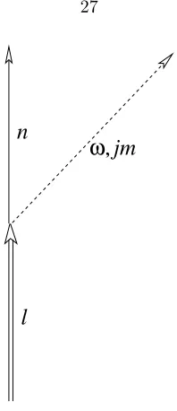
Figure 3.1: Feynman diagram of a first order S-matrix. Time flows forward in the upwards direction.
A nucleus is de-excited from state l to state n by emitting a photon of energy ¯hω and angular momentumjm.
nwith the emission of a photon) is3
S(1)=−ihωjm| hn|T
Z
V dt
|li (3.1)
wheren, lare indexes of the quantum system of the nucleus. The time-ordering operator is denoted byT.4 The angular momentum of the photon and its z component arej andm. The interaction
between a charged particle and a photon is5
V =
Z
ejµAµd3x (3.2)
where repetition of superscript and subscript indexes means summation. Here, jµ is the current 4-vector for the nucleus, which could be written as a bilinear term composed of the field operator of
3Actually, if one looks at a S-matrix element, e.g., the one in Eq. 3.1, one can find that it looks very much like a transition matrix elementhf|Ob|ii, whereidenotes the initial state andfthe final state,Obis a operator consisting of interaction potential.
4The time ordering operator greatly simplifies the formalisms in quantum field theories. 5One can convince oneself that this is reasonable by looking at the first term:Rej0A
the particle
jµ = ψ†γµψ (3.3)
ψ = Xcnφn (3.4)
The eigenstates of the Hamiltonian of the nucleus are{φn}. So we have
jµ =X nm
jµ
nmc†ncm (3.5)
where
jnmµ =φ∗nγµφm (3.6)
The photon field operator 6, A, which can be seen as the “wavefunction” of a photon, should be
expanded with photon “wavefunctions” of definite angular momentum,jm,
A=
Z
dω X
jm
aωjmχωjm+a†ωjmχ∗ωjm
(3.7)
A photon eigenstate of specific angular momentum,χωjm, is easier to write ink-space,
χωjm(k) = 4π2
ω3/2δ(|k| −ω)Yjm(n) (3.8)
which is basically the vector spherical harmonic function with proper normalization7. Its Fourier
transform defines the field in real space:
χωjm(x) =
Z
χωjm(k) exp (ik·x)
d3k
(2π)3 (3.9)
The orthogonality gives
1 2π
Z
χ∗ω0j0m0(x)χωjm(x)ω0ωd3x=ωδ(ω0−ω)δjj0δmm0 (3.10)
6A few more words about quantum electrodynamics: quantum electrodynamics is a quantum field theory, in which the field is quantized. We make the transition from classical mechanics to quantum mechanics by the quantization of physical quantities like position, momentum, Hamiltonian (so they are operators). A second quantization happens when we make the transition to quantum field theory, in which the wavefunctions become field operators.
After substituting Eqs. 3.2, 3.5 and 3.7 into Eq. 3.1, we found
in which we have explicitly written down the time evolution.
To further simplify this expression, recall
h|aωjma†ω0j0m0|i=δ(ω−ω0)δjj0δmm0 (3.12) The delta function signifies conservation of energy. The transition probability per unit time for such
a process is then8
dw
dt = 2πδ(En+ω−El)|Vnl;ωjm|
2
dω (3.17)
The result is natural since the transition probability increases as the interaction becomes stronger.
Integration over energy gives the transition probability per unit time accompanied by emission of
photons
dw
dt = 2π|Vnl;ωjm|
2
, where ω=El−En (3.18) which is just Fermi’s Golden Rule.
3.1.2
Interaction Matrix Element of Magnetic Transition
The interaction matrix element in Eq. 3.16 is the key to our problem. For57Fe M¨ossbauer
experi-ments, only the transition to the first excited state is important. This transition is of pure magnetic
dipole character. If we concern ourselves exclusively with magnetic transitions, the interaction
po-tential (cf. Landau and Lifshitz, QED, 2nd Edition, Pergamon Press, pg 171)
Vnl;ωjm= (−)mij is called the 2j-pole magnetic transition moment. We cannot obtain the value of this term without
detailed knowledge of the nucleus. For our isolated nucleus, however, the angular momentum is a
good quantum number, and we have
|li=|Ni |IMi (3.21)
where N denotes all quantum numbers except those of angular momentum, I and M are angular momentum and itsz component, respectively. Then with Wigner-Eckardt theorem9, one has
hn2I2M2|Q(j,m−)m|n1I1M1i=ij(−)Imax−M2
is the “reduced” transition matrix element, and
j2 j j1
−m2 −m m1
is the3j symbol. If we define a “reduced” interaction potential
Vn2I2←n1I1;ωj= (−)
The transition rate of an excited state is the sum of those of all possible transitions
ΓN,γ = 2π
l
n
n’
ω,
jm
ω
’, j’m’
Figure 3.2: Feynman diagram of a second-order S-matrix. Time flows forward in the upwards
direction. A nucleus of state|nicombines with a photon|ωjmiand forms a nucleus of state|li; it then de-excites to state|n0iby emitting a photon|ω0j0m0i.
= 2π
2IN+ 1|V0I0←LIN;ωjm|
2
(3.26)
where ω=EN−E0, j =IN −I0, m=MN−M0. Here, we use the subscriptγ to indicate that
this line-width of excited state is due to the electromagnetic radiation. Equation 3.26 relates the
transition rate of nuclear excited state resulted from radiation to the reduced interaction potential
defined in Eq. 3.23.
3.1.3
Scattering
Scattering of a Photon with Definite Angular Momentum
Consider the scattering of a photon by a fixed nucleus. The process can be regarded as three steps
(Fig. 3.2): 1. the nucleus gets excited from|nito|liby absorbing a photon; 2. the nucleus stays in state|lifor a while; 3. a photon is emitted while the nucleus jumps to state|n0i. The amplitude of
Using techniques similar to those in the previous Section, we obtain
Considering the commutation relations, the normalization conditions, and the unperturbed Green’s
function10 for the nucleus
G(0)(l, t−t0) =−i0DT Cl(t)Cl†(t0)
Here,l indicates the energy state of the nucleus
The sum overN can reduce to just one term if the energy levels of the nucleus are well-separated, compared to the energy line-width of the state. In our case, this is always true; the energy levels
are far apart, whereas the sublevels of an energy state are degenerate (e.g. Fe nucleus without an
external field), or very close to each other (e.g. hyperfine splittings of an Fe nucleus in an external
magnetic field). Thus, the sum overl reduces to a sum over sublevels of one excited state that is on resonance with the incidentγ-ray. At room temperature, essentially all nuclei are in their ground states, soN =N0= 0 (The quantum numberM
For elastic scattering,ω=ω0. For coherent elastic scattering, “spin-flip”-like phenomenon11does
not contribute. Thus, for coherent elastic scattering, we need to evaluate
hωjm| h0I0M0|S(2)|0I0M0i |ωjmi = −2πi
11For57Fe nucleus, the ground state is a spin 1
×G(0)(N INMN, E0I0M0+ω) (3.36)
In the last step, Eq. 3.26 was used. The amplitude of scattering process shown in Fig. 3.2 is related
to the line-width of nuclear excited state due to emmission ofγ-ray and the Green function of this state.
Beyond Second-Order Perturbation Theory
The previous derivations were only up to the second order in a perturbation expansion (S(2)). More
precise results can be obtained from QED: helping to justify this approach. With Feynman diagrams
we can see that higher order terms serve only to change the energy and the half-width of the excited
state of the nucleus. Actually the unperturbed Green’s function in, for example, Eq. 3.36 must be
replaced with the normal Green’s function
G(l, t−t0) =−iD
T Cl(t)Cl†(t0)
E. (3.37)
One example of high-order S-matrix is shown in Fig. 3.3.
More precisely, when all high-order S-matrixes are considered, both Eq. 3.18 and 3.35 need
revision. However, the net effect to Eq. 3.36 is only the replacement ofG(0) byG.12
Scattering Form Factor
Here we develop the scattering form factor. In formal scattering theory, the incident wave is treated
as a plane wave:
ψin=eik·r (3.38)
At a distance,r, far from the scattering center, the scattered wave is
ψsc=f(θ)e ik·r
r (3.39)
which is like a spherical wave, but with an angular dependency factor, f(θ), called the scattering amplitude. The scattering amplitude of a nuclear resonant scattering process is also called the form
factor for nuclear resonant scattering.
We need to evaluate how a plane wave photon (i.e., a photon with definite momentum) is scattered
Figure 3.3: An example of high-order S-matrix representing scattering process.
by a nucleus. The vector potential of such a photon could be described by|kαi
The amplitude of a process in which a photon with definite momentum is scattered by a nucleus
into a photon with definite angular momentum is then given by the S-matrix
hω0j0m0|h0I0M0|S|0I0M0i|kαi =
For coherent elastic scattering,
hω0j0m0|h0I0M0|S |0I0M0i|kαicoh,el = hω0j0m0|h0I0M0|S |0I0M0i|ω0j0m0i hω0j0m0|kαi
The problem now is to evaluate the projection coefficient between the photon state of definite angular
momentum and the photon states of definite momentum,hω0j0m0|kαi. First we note that using the
Thus for an incident plane wave, the scattered wave takes the form
Here N denotes the single energy level that is on resonance with the gamma ray energy, i.e., (EN−E0) ∼ ω ∼ ω0. j = IN −I0. The photon energy ω = |k|, direction n = kk. Equation
3.49 shows that the scattered wave is a photon state with definite angular momentum. To find
the scattering form factor, we need to express the scattered wave as a spherical wavef(θ)exp(rik·r), because, in formal scattering theory, the total wavefunction is the sum of Eq. 3.38 and 3.39
ψ = ψin+ψsc (3.51)
= eik·x+f(k)e ikr
r (3.52)
For the nuclear resonant scattering, the total photon wavefunction is
A(x) = S Ain(x) = (S(0)+S(2))Ain(x)
Now we want to know howAωjmbehaves whenkr1 (distance that is far away from the scattering center). Recall the well-know formula
and
Only the outgoing wave is relevant, so we have
In the second step the completeness of spherical harmonic functions is used. Thus,
Aout
After substituting Eq. 3.60 into Eq. 3.53 and compare it to Eq. 3.51, we obtained the form factor
f(ki,ei→kf,ef) = −
The Green’s function of a nucleus takes the form
G(l, E) = 1
E−(El−E0) +iΓl/2
. (3.63)
Here, the line-width Γl includes not only the contribution from radiation, but also contributions
from other transition channels, for example, the internal conversion, in which an inner shell electron
of an atom is emitted by the energy of nuclear transition. This means we must extend our analysis
from an isolated nucleus to a nucleus in an atom. Therefore, we have
×he(i)·Y∗jm(ni)
i h
e(f)∗·Yjm(nf)
i
|C(I0jIN;M0, m)|2 (3.65)
where the normalized energy shift is
zN,MN;0,M0(ω) = 2 ΓN
<