Robust Sentiment Detection on Twitter from Biased and Noisy Data

Robust Sentiment Detection on Twitter from Biased and Noisy Data

Luciano Barbosa

AT&T Labs - Research

[email protected]

Junlan Feng

AT&T Labs - Research

[email protected]

Abstract

In this paper, we propose an approach to automatically detect sentiments on Twit-ter messages (tweets) that explores some characteristics of how tweets are written and meta-information of the words that compose these messages. Moreover, we leverage sources of noisy labels as our training data. These noisy labels were provided by a few sentiment detection websites over twitter data. In our experi-ments, we show that since our features are able to capture a more abstract represen-tation of tweets, our solution is more ef-fective than previous ones and also more robust regarding biased and noisy data, which is the kind of data provided by these sources.

1 Introduction

Twitter is one of the most popular social network websites and has been growing at a very fast pace. The number of Twitter users reached an estimated 75 million by the end of 2009, up from approx-imately 5 million in the previous year. Through the twitter platform, users share either information or opinions about personalities, politicians, prod-ucts, companies, events (Prentice and Huffman, 2008) etc. This has been attracting the attention of different communities interested in analyzing its content.

Sentiment detection of tweets is one of the basic analysis utility functions needed by various appli-cations over twitter data. Many systems and ap-proaches have been implemented to automatically detect sentiment on texts (e.g., news articles, Web reviews and Web blogs) (Pang et al., 2002; Pang and Lee, 2004; Wiebe and Riloff, 2005; Glance et al., 2005; Wilson et al., 2005). Most of these

approaches use the raw word representation (n-grams) as features to build a model for sentiment detection and perform this task over large pieces of texts. However, the main limitation of using these techniques for the Twitter context is mes-sages posted on Twitter, so-called tweets, are very short. The maximum size of a tweet is 140 char-acters.

In this paper, we propose a 2-step sentiment analysis classification method for Twitter, which first classifies messages as subjective and ob-jective, and further distinguishes the subjective tweets as positive or negative. To reduce the la-beling effort in creating these classifiers, instead of using manually annotated data to compose the training data, as regular supervised learning ap-proaches, we leverage sources of noisy labels as our training data. These noisy labels were pro-vided by a few sentiment detection websites over twitter data. To better utilize these sources, we verify the potential value of using and combining them, providing an analysis of the provided labels, examine different strategies of combining these sources in order to obtain the best outcome; and, propose a more robust feature set that captures a more abstract representation of tweets, composed by meta-information associated to words and spe-cific characteristics of how tweets are written. By using it, we aim to handle better: the problem of lack of information on tweets, helping on the generalization process of the classification algo-rithms; and the noisy and biased labels provided by those websites.

combining these sources and present an extensive experimental evaluation in Section 4. Finally, we discuss previous works related to ours in Section 5 and conclude in Section 6, where we outline direc-tions and future work.

2 Preliminaries

In this section, we give some context about Twitter messages and the sources used for our data-driven approach.

Tweets. The Twitter messages are called tweets. There are some particular features that can be used to compose a tweet (Figure 1 illustrates an ex-ample): “RT” is an acronym for retweet, which means the tweet was forwarded from a previous post; “@twUser” represents that this message is a reply to the user “twUser”; “#obama” is a tag pro-vided by the user for this message, so-called hash-tag; and “http://bit.ly/9K4n9p” is a link to some external source. Tweets are limited to 140 charac-ters. Due to this lack of information in terms of words present in a tweet, we explore some of the tweet features listed above to boost the sentiment detection, as we will show in detail in Section 3.

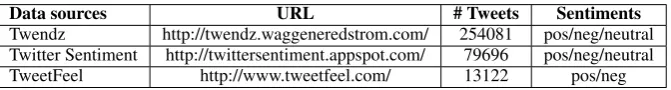
Data Sources. We collected data from 3 differ-ent websites that provide almost real-time sdiffer-enti- senti-ment detection for tweets: Twendz, Twitter Sen-timent and TweetFeel. To collect data, we issued a query containing a common stopword “of”, as we are interested in collecting generic data, and retrieved tweets from these sites for three weeks, archiving the returned tweets along with their sen-timent labels. Table 1 shows more details about these sources. Two of the websites provide 3-class detection: positive, negative and neutral and one of them just 2-class detection. One thing to note is our crawling process obtained a very dif-ferent number of tweets from each website. This might be a result of differences among their sam-pling processes of Twitter stream or some kind of filtering process to output. For instance, a site may only present the tweets it has more confi-dence about their sentiment. In Section 3, we present a deep analysis of the data provided by these sources, showing if they are useful to build a sentiment classification.

RT @twUser: Obama is the first U.S. president not to have seen a new state added in his lifetime. http://bit.ly/9K4n9p #obama

Figure 1: Example of a tweet.

3 Twitter Sentiment Detection

Our goal is to categorize a tweet into one of the three sentiment categories: positive, neutral or negative. Similar to (Pang and Lee, 2004; Wil-son et al., 2005), we implement a 2-step sentiment detection framework. The first step targets on dis-tinguishing subjective tweets from non-subjective tweets (subjectivity detection). The second one further classifies the subjective tweets into posi-tive and negaposi-tive, namely, the polarity detection. Both classifiers perform prediction using an ab-stract representation of the sentences as features, as we show later in this section.

3.1 Features

A variety of features have been exploited on the problem of sentiment detection (Pang and Lee, 2004; Pang et al., 2002; Wiebe et al., 1999; Wiebe and Riloff, 2005; Riloff et al., 2006) including un-igrams, bun-igrams, part-of-speech tags etc. A natu-ral choice would be to use the raw word represen-tation (n-grams) as features, since they obtained good results in previous works (Pang and Lee, 2004; Pang et al., 2002) that deal with large texts. However, as we want to perform sentiment detec-tion on very short messages (tweets), this strat-egy might not be effective, as shown in our ex-periments. In this context, we are motivated to develop an abstract representation of tweets. We propose the use of two sets of features: meta-information about the words on tweets and char-acteristics of how tweets are written.

Meta-features.Given a word in a tweet, we map it to its part-of-speech using a part-of-speech dic-tionary1_{. Previous approaches (Wiebe and Riloff,}

2005; Riloff et al., 2003) have shown that the ef-fectiveness of using POS tags for this task. The intuition is certain POS tags are good indica-tors for sentiment tagging. For example, opin-ion messages are more likely containing

adjec-1_{The pos dictionary we used in this paper is available at:}

Data sources URL # Tweets Sentiments

Twendz http://twendz.waggeneredstrom.com/ 254081 pos/neg/neutral Twitter Sentiment http://twittersentiment.appspot.com/ 79696 pos/neg/neutral TweetFeel http://www.tweetfeel.com/ 13122 pos/neg

Table 1: Information about the 3 data sources.

tives or interjections. In addition to POS tags, we map the word to its prior subjectivity (weak and strong subjectivity), also used by (Wiebe and Riloff, 2005), and polarity (positive, negative and neutral). The prior polarity is switched from pos-itive to negative or vice-versa when a negative expression (as, e.g., “don’t”, “never”) precedes the word. We obtained the prior subjectivity and polarity information from subjectivity lexicon of about 8,000 words used in (Riloff and Wiebe, 2003)2_{. Although this is a very comprehensive}

list, slang and specific Web vocabulary are not present on it, e.g., words as “yummy” or “ftw”. For this reason, we collected popular words used on online discussions from many online sources and added them to this list.

Tweet Syntax Features. We exploited the syn-tax of the tweets to compose our features. They are: retweet; hashtag; reply; link, if the tweet con-tains a link; punctuation (exclamation and ques-tions marks); emoticons (textual expression rep-resenting facial expressions); and upper cases (the number of words that starts with upper case in the tweet).

The frequency of each feature in a tweet is di-vided by the number of the words in the tweet.

3.2 Subjectivity Classifier

As we mentioned before, the first step in our tweet sentiment detection is to predict the subjectivity of a given tweet. We decided to create a single clas-sifier by combining the objectivity sentences from Twendz and Twitter Sentiment (objectivity class) and the subjectivity sentences from all 3 sources. As we do not know the quality of the labels pro-vided by these sources, we perform a cleaning process over this data to assure some reasonable quality. These are the steps:

1. Disagreement removal: we remove the

2_{The subjectivity lexicon is available at}

http://www.cs.pitt.edu/mpqa/

tweets that are disagreed between the data sources in terms of subjectivity;

2. Same user’s messages: we observed that the users with the highest number of messages in our dataset are usually those ones that post some objective messages, for example, ad-vertising some product or posting some job recruiting information. For this reason, we allowed in the training data only one message from the same user. As we show later, this boosts the classification performance, mainly because it removes tweets labeled as subjec-tive by the data sources but are in fact objec-tive;

3. Top opinion words: to clean the objective training set, we remove from this set tweets that contain the top-n opinion words in the subjectivity training set, e.g., words as cool, suck, awesome etc.

As we show in Section 4, this process is in fact able to remove certain noisy in the training data, leading to a better performing subjectivity classi-fier.

3.3 Polarity Classifier

The second step of our sentiment detection ap-proach is polarity classification, i.e., predict-ing positive or negative sentiment on subjective tweets. In this section, first we analyze the qual-ity of the polarqual-ity labels provided by the three sources, and whether their combination has the potential to bring improvement. Second, we present some modifications in the proposed fea-tures that are more suitable for this task.

3.3.1 Analysis of the Data Sources

The 3 data sources used in this work provide some kind of polarity labels (see Table 1). Two questions we investigate regarding these sources are: (1) how useful are these polarity labels? and (2) does combining them bring improvement in accuracy?

We take the following aspects into considera-tion:

• Labeler quality: if the labelers have low qual-ity, combine them might not bring much im-provement (Sheng et al., 2008). In our case, each source is treated as a labeler;

• Number of labels provided by the labelers: if the labels are informative, i.e., the prob-ability of them being correct is higher than 0.5, the more the number of labels, the higher is the performance of a classifier built from them (Sheng et al., 2008);

• Labeler bias: the labeled data provided by the labelers might be only a subset of the real data distribution. For instance, labelers might be interested in only providing labels that they are more confident about;

• Different labeler bias: if labelers make simi-lar mistakes, the combination of them might not bring much improvement.

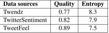
We provide an empirical analysis of these datasets to address these points. First, we measure the polarity detection quality of a source by calcu-lating the probabilitypof a label from this source being correct. We use the data manually labeled for assessing the classifiers’ performance (testing data, see Section 4) to obtain the correct labels of

Data sources Quality Entropy

Twendz 0.77 8.3

TwitterSentiment 0.82 7.9 TweetFeel 0.89 7.5

Table 2: Quality of the labels and entropy of the tweets provided by each data source for the polar-ity detection.

a data sample. Table 2 shows their values. We can conclude from these numbers that the 3 sources provide a reasonable quality data. This means that combining them might bring some improvement to the polarity detection instead of, for instance, using one of them in isolation. An aspect that is overlooked by quality is the bias of the data. For instance, by examining the data from TwitterFeel, we found out that only 4 positive words (“awe-some”,“rock”,“love” and “beat”) cover 95% of their positive examples and only 6 negative words (“hate”,“suck”,“wtf”,“piss”,“stupid” and “fail”) cover 96% of their negative set. Clearly, the data provided by this source is biased towards these words. This is probably the reason why this web-site outputs such fewer number of tweets com-pared to the other websites (see Table 1) as well as why its data has the smallest entropy among the sources (see Table 2).

Data sources Kappa

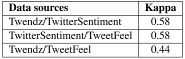
Twendz/TwitterSentiment 0.58 TwitterSentiment/TweetFeel 0.58 Twendz/TweetFeel 0.44

Table 3: Kappa coefficient between pairs of sources.

From this analysis we can conclude that com-bining the labels provided by the 3 sources can improve the performance of the polarity detec-tion instead of using one of them in isoladetec-tion be-cause they provide diverse labels (moderate kappa agreement) of reasonable quality, although there is some issues related to bias of the labels pro-vided by them. In our experimental evaluation in Section 4, we present results obtained by different strategies of combining these sources that confirm these findings.

3.3.2 Polarity Features

The features used in the polarity detection are the same ones used in the subjectivity detection. However, as one would expect the set of the most discriminative features is different between the two tasks. For subjectivity detection, the top-5 features in terms of information gain, based on the training data, are: negative polarity, positive polarity, verbs, good emoticons and upper case. For this task, the meta-information of the words (negative polarity, positive polarity and verbs) is more important than specific features from Twitter (good emoticons and upper case), whereas for the subjectivity detection, tweet syntax features have a higher relevance.

This analysis show that prior polarity is very important for this task. However, one limitation of using it from a generic list is its values might not hold for some specific scenario. For instance, the polarity of the word “spot” is positive accord-ing to this list. However, lookaccord-ing at our trainaccord-ing data almost half of the occurrences of this word appears in the positive set and the other half in the negative set. Thus, it is not correct to as-sume that prior polarity of “spot” is 1 for this particular data. This example illustrates our strat-egy to weight the prior polarities: for each word

w with prior polarity defined by the list, we

cal-culate the prior polarity of w, pol(w), based on the distribution ofwin the positive and negative sets. Thus, polpos(w) =count(w,pos)/count(w)

and polneg(w) =1−polpos(w). We assume the

polarity of a word is associated with the polar-ity of the sentence, which seems to be reasonable since we are dealing with very short messages. Although simple, this strategy is able to improve the polarity detection, as we show in Section 4.

4 Experiments

We have performed an extensive performance evaluation of our solution for twitter sentiment detection. Besides analyzing its overall perfor-mance, our goals included: examining different strategies to combine the labels provided by the sources; comparing our approach to previous ones in this area; and evaluating how robust our solu-tion is to the noisy and biased data described in Section 3.

4.1 Experimental Setup

Data Sets. For the subjectivity detection, after the cleansing processing (see Section 3), the train-ing data contains about 200,000 tweets (roughly 100,000 tweets were labeled by the sources as subjective ones and 100,000 objective ones), and for polarity detection, 71046 positive and 79628 negative tweets. For test data, we manually la-beled 1,000 tweets as positive, negative and neu-tral. We also built a development set (1,000 tweets) to tune the parameters of the classification algorithms.

Approaches. For both tasks, subjectivity and po-larity detection, we compared our approach with previous ones reported in the literature. Detailed explanation about them are as follows:

compose the sentences. We used the imple-mentation provided by LingPipe (LingPipe, 2008);

• Unigrams: Pang et al. (Pang et al., 2002) showed unigrams are effective for sentiment detection in regular reviews. Based on that, we built unigram-based classifiers for the subjectivity and polarity detections over the training data. Another approach that uses un-igrams is the one used by TwitterSentiment website. For polarity detection, they select the positive examples for the training data from the tweets containing good emoticons and negative examples from tweets contain-ing bad emoticons. (Go et al., 2009). We built a polarity classifier using this approach (Unigrams-TS).

• TwitterSA: TwitterSA exploits the features described in Section 3 in this paper. For the subjectivity detection, we trained a clas-sifier from the two available sources, us-ing the cleanus-ing process described in Sec-tion 3 to remove noise in the training data, TwitterSA(cleaning), and other classifier trained from the original data, TwitterSA(no-cleaning). For the polarity detection task, we built a few classifiers to compare their performances: TwitterSA(single) and Twit-terSA(weights) are two classifiers we trained using combined data from the 3 sources. The only difference is TwitterSA(weights) uses the modification of weighting the prior polarity of the words based on the train-ing data. TwitterSA(voting) and Twit-terSA(maxconf) combine classification out-puts from 3 classifiers respectively trained from each source. TwitterSA(voting) uses majority voting to combine them and Twit-terSA(maxconf) picks the one with maxi-mum confidence score.

We use Weka (Witten and Frank, 2005) to cre-ate the classifiers. We tried different learning al-gorithms available on Weka and SVM obtained the best results for Unigrams and TwitterSA. Ex-perimental results reported in this section are ob-tained using SVM.

4.2 Subjectivity Detection Evaluation

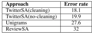
Table 4 shows the error rates obtained by the dif-ferent subjectivity detection approaches. Twit-terSA achieved lower error rate than both Uni-grams and ReviewSA. As a result, these num-bers confirm that features inferred from meta-information of words and specific syntax features from tweets are better indicators of the subjectiv-ity than unigrams. Another advantage of our ap-proach is since it uses only 20 features, the train-ing and test times are much faster than ustrain-ing thou-sands of features like Unigrams. One of the rea-sons why TwitterSA obtained such a good perfor-mance was the process of data cleansing (see Sec-tion 3). The label quality provided by the sources for this task was very poor: 0.66 for Twendz and 0.68 for TwitterSentiment. By cleaning the data, the error decreased from 19.9, TwitterSA(no-cleaning), to 18.1, TwitterSA(cleaning). Regard-ing ReviewSA, its lower performance is expected since tweets are composed by single sentences and ReviewSA relies on the proximity between sentences to perform subjectivity detection.

We also investigated the influence of the size of training data on classification performance. Fig-ure 2 plots the error rates obtained by TwitterSA and Unigrams versus the number of training ex-amples. The curve corresponding to TwitterSA showed that it achieved good performances even with a small training data set, and kept almost con-stant as more examples were added to the train-ing data, whereas for Unigrams the error rate de-creased. For instance, with only 2,000 tweets as training data, TwitterSA obtained 20% of error rate whereas Unigrams 34.5%. These numbers show that our generic representation of tweets produces models that are able to generalize even with a few examples.

4.3 Polarity Detection Evaluation

cre-ated from a single training data. This result shows that computing the prior polarity of the words based on the training data TwitterSA(weights) brings some improvement for this task. Twit-terSA(voting) obtained the highest error rate among the TwitterSA approaches. This implies that, in our scenario, the best way of combining the merits of the individual classifiers is by using a confidence score approach.

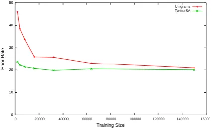
Unigrams also achieved comparable perfor-mances. However, when reducing the size of the training data, the performance gap between Twit-terSA and Unigrams is much wider. Figure 3 shows the error rate of both approaches3_in

func-tion of the training size. Similar to subjectivity de-tection, the training size does not have much influ-ence in the error rate for TwitterSA. However for Unigrams, it decreased significantly as the train-ing size increased. For instance, for a traintrain-ing size with 2,000 tweets, the error rate for Unigrams was 46% versus 23.8% for our approach. As for subjectivity detection, this occurs because our fea-tures are in fact able to capture a more general rep-resentation of the tweets.

Another advantage of TwitterSA over Uni-grams is that it produces more robust models. To illustrate this, we present the error rates of Uni-grams and TwitterSA where the training data is composed by data from each source in isolation. For the TweetFeel website, where data is very bi-ased (see Section 3), Unigrams obtained an error rate of 44.5% whereas over a sample of the same size of the combined training data (Figure 3), it obtained an error rate of around 30%. Our ap-proach also performed worse over this data than the general one, but still had a reasonable er-ror rate, 25.1%. Regarding the Twendz website, which is the noisiest one (Section 3), Unigrams also obtained a poor performance comparing it against its performance over a sample of the gen-eral data with a same size (see Table 5 and Fig-ure 3). Our approach, on the other hand, was not much influenced by the noise (22.9% on noisy data and around 20% on the sample of same size of the general data). Finally, since the data qual-ity provided by TwitterSentiment is better than the

3_{For this experiment, we used the TwitterSA(single)}

con-figuration.

Approach Error rate

TwitterSA(cleaning) 18.1 TwitterSA(no-cleaning) 19.9

Unigrams 27.6

ReviewSA 32

Table 4: Results for subjectivity detection.

Approach Error rate

TwitterSA(maxconf) 18.7 TwitterSA(weights) 19.4 TwitterSA(single) 20 TwitterSA(voting) 22.6

Unigrams 20.9

ReviewSA 21.7

Unigrams-TS 24.3

Table 5: Results for polarity detection.

Site Training Size TwitterSA Unigrams

TweetFeel 13120 25.1 44.5 Twendz 78025 22.9 32.3 TwitterSentiment 59578 22 23.4

Table 6: Training data size for each source and error rates obtained by classifiers built from them.

0 5 10 15 20 25 30 35 40

0 20000 40000 60000 80000 100000 120000 140000 160000 180000 200000

Error Rate

Training Size

Unigrams TwitterSA

Figure 2: Influence of the training data size in the error rate of subjectivity detection using Unigrams and TwitterSA.

previous sources (Table 2), there was not much impact over both classifiers created from it.

0 10 20 30 40 50

0 20000 40000 60000 80000 100000 120000 140000 160000

Error Rate

Training Size

Unigrams TwitterSA

Figure 3: Influence of the training data size in the error rate of polarity detection using Unigrams and TwitterSA.

5 Related Work

There is a rich literature in the area of sentiment detection (see e.g., (Pang et al., 2002; Pang and Lee, 2004; Wiebe and Riloff, 2005; Go et al., 2009; Glance et al., 2005). Most of these ap-proaches try to perform this task on large texts, as e.g., newspaper articles and movie reviews. An-other common characteristic of some of them is the use of n-grams as features to create their mod-els. For instance, Pang and Lee (Pang and Lee, 2004) explores the fact that sentences close in a text might share the same subjectivity to create a better subjectivity detector and, similar to (Pang et al., 2002), uses unigrams as features for the polar-ity detection. However, these approaches do not obtain a good performance on detecting sentiment on tweets, as we showed in Section 4, mainly be-cause tweets are very short messages. In addition to that, since they use a raw word representation, they are more sensible to bias and noise, and need a much higher number of examples in the train-ing data than our approach to obtain a reasonable performance.

The Web sources used in this paper and some other websites provide sentiment detection for tweets. A great limitation to evaluate them is they do not make available how their classification was built. One exception is TwitterSentiment (Go et al., 2009), for instance, which considers tweets with good emoticons as positive examples and tweets with bad emoticons as negative examples for the training data, and builds a classifier using

unigrams and bigrams as features. We showed in Section 4 that our approach works better than theirs for this problem, obtaining lower error rates.

6 Conclusions and Future Work

We have presented an effective and robust sen-timent detection approach for Twitter messages, which uses biased and noisy labels as input to build its models. This performance is due to the fact that: (1) our approach creates a more abstract representation of these messages, instead of using a raw word representation of them as some pre-vious approaches; and (2) although noisy and bi-ased, the data sources provide labels of reasonable quality and, since they have different bias, com-bining them also brought some benefits.

The main limitation of our approach is the cases of sentences that contain antagonistic sentiments. As future work, we want to perform a more fine grained analysis of sentences in order to identify its main focus and then based the sentiment clas-sification on it.

References

Cohen, J. 1960. A coefficient of agreement for nomi-nal scales.Educational and psychological measure-ment, 20(1):37.

Glance, N., M. Hurst, K. Nigam, M. Siegler, R. Stock-ton, and T. Tomokiyo. 2005. Deriving marketing intelligence from online discussion. In Proceed-ings of the eleventh ACM SIGKDD, pages 419–428. ACM.

Go, A., R. Bhayani, and L. Huang. 2009. Twit-ter sentiment classification using distant supervi-sion. Technical report, Stanford Digital Library Technologies Project.

Landis, J.R. and G.G. Koch. 1977. The measurement of observer agreement for categorical data. Biomet-rics, pages 159–174.

LingPipe. 2008. LingPipe 3.9.1. http://alias-i.com/lingpipe.

Pang, B., L. Lee, and S. Vaithyanathan. 2002. Thumbs up?: sentiment classification using machine learn-ing techniques. In Proceedings of the ACL, pages 79–86. Association for Computational Linguistics.

Polikar, R. 2006. Ensemble based systems in deci-sion making. IEEE Circuits and systems magazine, 6(3):21–45.

Prentice, S. and E. Huffman. 2008. Social Medias New Role In Emergency Management. Idaho Na-tional Laboratory, pages 1–5.

Riloff, E. and J. Wiebe. 2003. Learning extraction pat-terns for subjective expressions. InProceedings of the 2003 conference on Empirical methods in natu-ral language processing, pages 105–112.

Riloff, E., J. Wiebe, and T. Wilson. 2003. Learning subjective nouns using extraction pattern bootstrap-ping. InProceedings of the 7th Conference on Nat-ural Language Learning, pages 25–32.

Riloff, E., S. Patwardhan, and J. Wiebe. 2006. Feature subsumption for opinion analysis. InProceedings of the 2006 Conference on Empirical Methods in Natural Language Processing, pages 440–448. As-sociation for Computational Linguistics.

Sheng, V.S., F. Provost, and P.G. Ipeirotis. 2008. Get another label? Improving data quality and data min-ing usmin-ing multiple, noisy labelers. InProceeding of the 14th ACM SIGKDD international conference on Knowledge discovery and data mining, pages 614– 622. ACM.

Wiebe, J. and E. Riloff. 2005. Creating subjective and objective sentence classifiers from unannotated texts. Computational Linguistics and Intelligent Text Processing, pages 486–497.

Wiebe, J.M., RF Brace, and T.P. O’Hara. 1999. Devel-opment and use of a gold-standard data set for sub-jectivity classifications. InProceedings of the ACL, pages 246–253. Association for Computational Lin-guistics.

Wilson, T., J. Wiebe, and P. Hoffmann. 2005. Rec-ognizing contextual polarity in phrase-level senti-ment analysis. In EMNLP, page 354. Association for Computational Linguistics.