Algebraic Companions and Linearizations

(1)

Scholarship@Western

Electronic Thesis and Dissertation Repository

8-23-2019 9:30 AM

Algebraic Companions and Linearizations

Eunice Y. S. Chan

The University of Western Ontario

Supervisor

Corless, Robert M.

The University of Western Ontario

Graduate Program in Applied Mathematics

A thesis submitted in partial fulfillment of the requirements for the degree in Doctor of Philosophy

Follow this and additional works at: https://ir.lib.uwo.ca/etd

Part of the Numerical Analysis and Computation Commons

Recommended Citation Recommended Citation

Chan, Eunice Y. S., "Algebraic Companions and Linearizations" (2019). Electronic Thesis and Dissertation Repository. 6414.

https://ir.lib.uwo.ca/etd/6414

This Dissertation/Thesis is brought to you for free and open access by Scholarship@Western. It has been accepted for inclusion in Electronic Thesis and Dissertation Repository by an authorized administrator of

(2)

Abstract

In this thesis, we look at a novel way of finding roots of a scalar polynomial using eigenvalue techniques. We extended this novel method to the polynomial eigenvalue problem (PEP). PEP have been used in many science and engineering applications such vibrations of structures, computer-aided geometric design, robotics, and machine learning. This thesis explains this idea in the order which we discovered it.

In Chapter 2, a new kind of companion matrix is introduced for scalar polynomials of the formc(λ) = λa(λ)b(λ)+c0, where upper Hessenberg companions are known for the

polyno-mialsa(λ) andb(λ). This construction can generate companion matrices with smaller entries

than the Fiedler or Frobenius forms. This generalizes Piers Lawrence’s Mandelbrot companion matrix. The construction was motivated by use of Narayana-Mandelbrot polynomials.

In Chapter 3, we define Euclid polynomials Ek₊1(λ)= Ek(λ)(Ek(λ)−1)+1 whereE1(λ)=

λ+1 in analogy to Euclid numbersek = Ek(1). We show how to construct companion matrices

Ek, soEk(λ)=det(λI−Ek) is of height 1 (and thus of minimal height over all integer compan-ion matrices for Ek(λ)). We prove various properties of these objects, and give experimental

confirmation of some unproved properties.

In Chapter 4, we show how to construct linearizations of matrix polynomialsza(z)d0+ c0,

a(z)b(z), a(z)+ b(z) (when deg(b(z)) < deg(a(z))), and za(z)d0b(z)+ c0 from linearizations

of the component parts, matrix polynomials a(z) and b(z). This extends the new companion matrix construction introduced in Chapter 2 to matrix polynomials.

In Chapter 5, we define “generalized standard triples” which can be used in constructing algebraic linearizations; for example, for H(z) = za(z)b(z)+ c0 from linearizations for a(z)

and b(z). For convenience, we tabulate generalized standard triples for orthogonal polyno-mial bases, the monopolyno-mial basis, and Newton interpolational bases; for the Bernstein basis; for Lagrange interpolational bases; and for Hermite interpolational bases. We account for the possibility of common similarity transformations. We give explicit proofs for the less familiar bases.

In Chapter 6, we investigate the numerical stability of algebraic linearization, which re-uses linearizations of matrix polynomials a(λ) and b(λ) to make a linearization for the matrix poly-nomial P(λ) =λa(λ)b(λ)+c. Such a re-useseemsmore likely to produce a well-conditioned linearization, and thus the implied algorithm for finding the eigenvalues ofP(λ) seems likely to be more numerically stable than expanding out the product a(λ)b(λ) (in whatever polynomial basis one is using). We investigate this question experimentally by using pseudospectra.

Keywords: matrix, polynomial, matrix polynomial, linearizations, pseudospectra, Bo-hemian, companion matrix, comrade matrix, eigenvalues

(3)

Matrix polynomials have been used in many scientific and engineering applications, ranging from vibrations of structures including buildings and aircrafts to machine learning. This thesis studies new and effective methods for solving design problems with such models. This thesis provides new theory and new algorithms. We introduce several new ideas including minimal height companion matrices which promise more numerically stable algorithms. A numerically stable algorithm gives exact solutions to a nearby problem. This thesis extends this result to the case where the polynomial coefficients are matrices themselves i.e. matrix polynomials.

(4)

Co-Authorship Statement

This integrated-article thesis is based on 5 papers. A version of Chapter 2 [1] has been published; in this thesis, an addition has been made at the end of section 4.3. Chapters 3 [2], and 4 [3] have been published in academic journals. Chapter 5 has been submitted for publi-cation. Chapter 6 is being prepared for publipubli-cation. For these papers, Robert Corless provided assistance with the theoretical understanding of companion matrices and linearizations, and provided feedback on the papers. The initial basis for chapter 4 was developed by Robert Cor-less, Laureano Gonzalez-Vega, J. Rafael Sendra, and Juana Sendra. Rob provided assistance with the main proofs in Section 4.3. Leili Rafiee Sevyeri provided assistance with the Bernstein basis section of Chapter 5.

Bibliography

[1] E. Y. S. Chan andR. M. Corless, A new kind of companion matrix, Electronic Journal of Linear Algebra, 32 (2017), pp. 335–342.

[2] , Minimal height companion matrices for Euclid polynomials, Mathematics in Com-puter Science, 13 (2019), pp. 41–56.

[3] E. Y. S. Chan, R. M. Corless, L. Gonzalez-Vega, J. R. Sendra,andJ. Sendra, Algebraic

linearizations for matrix polynomials, Linear Algebra and its Applications, 563 (2019), pp. 373–399.

(5)

I am very grateful for the support that I have received from many people during my graduate studies. Below are the people that I am especially grateful for and without them, this thesis may not have been possible.

First, without my supervisor Robert Corless, this thesis most definitely would not have been possible. I would like to thank Rob for giving me the opportunity to learn and grow as a researcher from him—I would not have become the researcher I am today without his guidance. I also would like to thank Rob for his generosity, time, and encouragement while under his supervision.

Secondly, I would like to thank my parents, Mei Po Wong and Charm Fung Chan, and my brother, Sunny Chan for their constant support, especially through graduate school.

Thirdly, I would like to thank Janet Martin for allowing me the opportunity to apply my mathematical and programming knowledge to the field of public health.

Fourthly, I would like to thank my Spanish colleague and co-authors Laureano Gonzalez-Vega, J. Rafael Sendra, and Juana Sendra for their tremendous generosity during my visit in Spain during my last semester of my PhD.

Lastly, I would like to thank the professors and staffin the Department of Applied Mathe-matics for their help during my graduate studies.

(6)

List of Figures

2.1 Roots of Narayana-Mandelbrot polynomial, r36(z). The degree of r36(z) is

578,948. . . 14

3.1 All 16,384 roots of the Euclid polynomialE15(λ) with circle of radius 1.1180,

the approximate magnitude of the largest|λ+1/₂_|_{. . . 25}

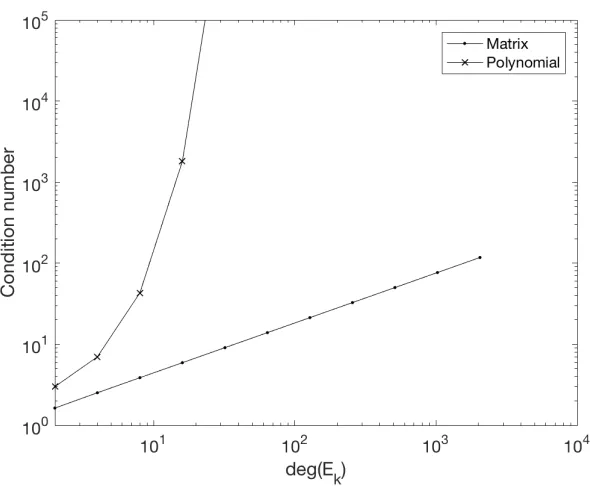
3.2 Log-log plot of condition numbers of the evaluation of the Euclid polynomials and the 2-norm condition number of their companions from k = 2 to k =

12. The computed slope for the condition number for the matrices is 0.618 giving an estimated condition number growth as Ke ∼ d0.618 which is better than the expectedO(d2) behaviour [1]. The curious three digit coincidence with

(√5−1)/2is noted. The doubly exponential growth of the polynomial conditioning

appears as exponential growth in this log log plot. . . 28 3.3 The similar spacings between Figures 3.3a, 3.3b and 3.3c demonstrate the

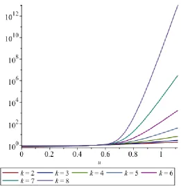
su-perior conditioning of the companion matrix, owing to its minimal height. . . . 30 3.4 Condition numbers for the evaluation of Ek(λ) eBk(u) on 0 ≤ u ≤ 1.1180 for

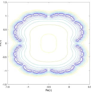
k=2 to 8. . . 32 3.5 Pseudospectra of _E8 for 10 logarithmically-spaced values of ε between 10−2

and 10−1. . . 33

4.1 Eigenvalues of a 4092×4092 matrix. For details, refer to equation (4.6) . . . . 51 4.2 Matrix structure of the companion matrix (H,DH) ofh(z)=za(z)b(z)+c0. The

block of zeros inDH means that there are spurious infinite eigenvalues. These are numerically harmless and can be discarded. . . 56

6.1 Pseudospectra of (6.5) to demonstrate the connection between pseudospectra and backward stability. The length of the line connecting the eigenvalue (λ =

2.23) and the contour ( =0.05) is the forward error. . . 97 6.2 Pseudospectra of two different linearizations (left: algebraic linearization, right:

frobenius linearization) of the matrix polynomial in the form λa(λ)b(λ)+ c0

given in equation (6.5). . . 99 6.3 Pseudospectra of two different kinds of linearizations for equation (6.5) which

is expressed in the monomial basis. The linearization constructions used are algebraic linearization (left) and Frobenius linearization (right). . . 100 6.4 Pseudospectra of two different kinds of linearizations for equation (6.6) which

is expressed in the monomial basis. The linearization constructions used are algebraic linearization (left) and Frobenius linearization (right). . . 101

(10)

6.5 The left figure uses the form in (6.7) and uses algebraic linearizations to con-struct the companion. The center figure expresses the inner termsλA(λ)B(λ)+ c0andλC(λ)D(λ)+c1in the monomial basis. This is so that we use the

Frobe-nius linearization construction for the parts expressed in the monomial basis and then use algebraic linearization to construct the final companion. Lastly, we use the expanded form of the equation and created the Frobenius lineariza-tion (right). . . 102 6.6 Pseudospectra of two different kinds of linearizations for equation – which is

expressed in the Bernstein basis. The linearization constructions used are alge-braic linearization (left), linearization for matrix polynomials expressed in the Bernstein basis (center), Frobenius linearization (right). . . 103 6.7 Pseudospectra for equation (6.9) which is expressed in various ways. The

lin-earization constructions used are algebraic linlin-earization (left) and the Frobenius linearization for matrix polynomials expressed in the monomial basis (right). . . 104

(11)

List of Tables

3.1 Pseudozeros/pseudospectra of Ek(λ), Ek(u) and _Ek for k = 6,7,8. For these

ε ranges, the pictures are similar to those of Figure 3.3. These pictures are available upon request. . . 31

4.1 Times of eigenvalue computation of the algebraic linearizations using Maple. The polynomial solverfsolve takes so long because the heights of the char-acteristic polynomials grow exponentially in the dimension. The eigenvalue solver has no difficulty, because the matrix height is constant. . . 52

5.1 A short list of three-term recurrence relations for some important polynomial bases. For a more comprehensive list, see The Digital Library of Mathematical Functions. These relations and others are coded in Walter Gautschi’s packages OPQ and SOPQ [15] and in theMatrixPolynomialObject implementation package in Maple (see [19]). . . 65

(12)

Chapter 1 Introduction

For this thesis, we are interested in finding solutions to univariate scalar and matrix polynomial problems numerically. To solve for the zeros in the scalar case, we convert the polynomial problem into an eigenvalue problem, where we build a matrix whose eigenvalues are nearly identical to the solution of the polynomial problem. Such a matrix is called a companion ma-trix. Rather than using commonly-used constructions such as Frobenius [1] and Fiedler [2], we introduce a new construction for the companion matrix, first thought of by Piers W. Lawrence for the Mandelbrot matrices. We generalized his construction for polynomials in the form

p(z)= za0(z)·a1(z)· · ·an(z)+c,

wherenis an integer greater than 0,ai(z) are scalar polynomials with deg(ai(z))> 0, andc∈_C. We then extended this construction to the matrix polynomials that were in the form

P(λ)= λa(λ)b(λ)+c, (1.1)

where a(λ) and b(λ) are matrix polynomials expressed in any polynomial basis with their coefficients of the same dimension _Cr×r_{, and} _c _∈

Cr×r. In this case, instead of calling the

matrix a companion, we use the term linearization as it is conventional.

This chapter breaks down the scalar polynomial problem and the polynomial eigenvalue problem, separately, and then gives an outline of this thesis.

1.1 Finding solutions to a scalar polynomial

Polynomial system models are used extremely frequently in mathematics, engineering, and science. These systems have been studied extensively, such computer aided geometric design by Sederberg [7] and robotics by Sommese and Wampler [8]. In the first part of this thesis, we focus on univariate scalar polynomials.

A scalar polynomial expressed in the monomial basis is defined by

A(z)=

n

X

i=0

ziai, ai ∈_C, an_, 0.

The article [5] surveys efficient methods to solve these polynomials, ranging from iterative methods to multi-point methods to methods based on rational approximation and more. One

(13)

method that we are particularly interested in is to solve for the roots of a scalar polynomial is to convert the problem into an eigenvalue problem. The most popular construction is the Frobenius companion. The generalized companion matrix construction is

M1(z)= z

                 

an 0 · · · 0

0 1 0 ... ... 0 ... 0 0 · · · 0 1                   −                 

−an−1 −an−2 · · · −a0

1 0 · · · 0

0 ... ... ...

0 0 1 0

                 , (1.2)

where det (M1(z))= A(z). The permutations of equation (1.2),

M2(z)=z

                 

1 0 · · · 0

0 ... 0 ... ... 0 1 0 0 · · · 0 an

                  −                 

1 0 · · · 0

0 ... ... ...

0 0 1 0

−a0 −a1 · · · −an−1

                

M3(z)=z

                 

1 0 · · · 0

0 ... 0 ... ... 0 1 0 0 · · · 0 an

                  −                  

0 · · · 0 −a0

1 ... ... −a1

0 ... 0 ... 0 0 1 −an−1

                 

M4(z)=z

                 

an 0 · · · 0

0 1 0 ... ... 0 ... 0 0 · · · 0 1                   −                  

−an−1 1 0 0

−an−2 0 ... 0

... ... ... 1 −a0 0 · · · 0

                 

are also commonly used. Although the Frobenius construction is the most popular, there are many other companion matrix constructions, such as the Fiedler construction and the construc-tion that we will introduce in this thesis. Companion matrices are sometimes referred to as comrade matrices or colleague matrices.

The polynomial that we are interested in is in the recursive form

p(z)= za(z)b(z)+c.

Our construction (Theorem 2.2.1) takes advantage of this form: if we know the companions fora(z) andb(z), we can simply “glue” everything together, creating the companion forp(z).

We can show through a small example why it may be advantageous to use our companion matrix construction rather than the Frobenius companion matrix construction. Let us take

p(z)= z(z+1)(z+1)+1 (1.3)

(14)

1.1. Finding solutions to a scalar polynomial 3

Using Maple 2017, we can find the roots exactly:

−1 6 3 q

100+12 √

69− 2 3

1

3 q

100+12√69 − 2 3 , 1 12 3 q

100+12 √

69+ 1 3

1

3 q

100+12√69 − 2 3 + i 2 √ 3             −1 6 3 q

100+12 √

69+ 2 3

1

3 q

100+12√69             , 1 12 3 q

100+12 √

69+ 1 3

1

3 q

100+12√69 − 2 3 − i 2 √ 3             −1 6 3 q

100+12 √

69+ 2 3

1

3 q

100+12√69             ,

which evaluated using 20 digit precision are

−1.7548776662466927601,

−0.12256116687665361998−0.74486176661974423660i,

−0.12256116687665361998+0.74486176661974423660i,

respectively.

The Frobenius companion matrix for this example would be

zI3−

         

−2 −1 −1

1 0 0

0 1 0

          . (1.5)

The characteristic polynomial of equation (1.5) is

z+2 1 1

−1 z 0

0 −1 z

=(z+2) z 0

−1 z

+ 1 1 −1 z

=z2(z+2)+z+1

=z3+2z2+z+1,

which is equivalent to equation (1.4), which means that the eigenvalues of equation (1.5) are the solutions to equation (1.4) if computed exactly. Using MatlabR2017a’seigroutine, the eigenvalues of equation (1.5) are

−1.754877666246694+0.000000000000000i

−0.122561166876654+0.744861766619744i

−0.122561166876654−0.744861766619744i.

On the other hand, our companion matrix for this example would be

zI3−

         

−1 0 −1

−1 0 0

(15)

The characteristic polynomial of (1.6) is

z+1 0 1

1 z 0

0 1 z+1

= (z+1)

z 0

1 z+1

−

0 1 1 z+1

= (z+1)z(z+1)+1

= z(z+1)2+1

= z3+2z2+z+1,

which is also equivalent to equation (1.4) meaning that equation (1.6) is also a companion of (1.4). Using Matlab’seigroutine, the eigenvalues of equation (1.6) are

−1.754877666246691+0.000000000000000i

−0.122561166876653+0.744861766619744i

−0.122561166876653−0.744861766619744i.

We can see that the eigenvalues of both companions are slightly different than the solution eval-uated by Maple. This demonstrates the idea of “solving the exact solution to a nearby problem”, thus resulting in nearly identical results. On another note, even though this is a small example, we can see that equation (1.6) has lower height compared to equation (1.5) since our con-struction does not require the multiplication between coefficients. Lower height becomes more important for larger problems by offering smaller condition number of the eigenvalues, which suggests better backward stability. We demonstrate this by using pseudospectra in chapters 3 and 6.

1.2 Polynomial eigenvalue problem

For the matrix polynomial case, polynomial eigenvalue problems (PEP) arise in many applica-tions. In Mackey et al. [4], the authors mention applications in extreme designs, such as high speed trains, optoelectronic devices, micro-electromechanical systems and “superjumbo” jets such as the Airbus 380. This particular application presents a challenge for the computation of the resonant frequencies of these structures since these extreme designs often lead to eigen-problems with poor conditioning. Other applications of PEP can be found in survey articles such as G¨uttel and Tisseur [3] and Mehrmann and Voss [6].

The polynomial eigenvalue problem is to find scalars λand nonzero vectors xandy satis-fying P(λ)x=0 and y∗P(λ)= _{0 where}

P(λ)=

m

X

i=0

φi(λ)Ai, Ai ∈Cn×n, Am, 0

is a matrix polynomial of degreemandφi(λ) is any polynomial basis. If detP(λ) is not a zero

polynomial, then the matrix polynomial is regular. For matrix polynomials expressed in the power basis, when Amis the identity matrix, the matrix polynomial is classified as a monicn×n

(16)

1.3. Outline 5

identity matrix or even invertible, but not identically equal to zero, then the matrix polynomial is classified as a non-monicn×nmatrix polynomial. Chapters 4 to 6 consider these cases in various polynomial bases. Chapter 6 also gives an example where the leading coefficient of the matrix polynomial is singular.

The standard way of solving this problem is bylinearization, where we convert the matrix polynomial P(λ) into a linear polynomial

L(λ)= λC1+C0

whereC0, C1 ∈ Cmn×mn, whose eigenvalues are nearly identical to the solution of the matrix

polynomial. It is guaranteed that both P(λ) and L(λ) have the same spectrum if

E(λ)L(λ)F(λ)=

"_P(λ) 0 0 I(m−1)n

#

where E(λ) and F(λ) are unimodular. Chapter 5 presents the linearizations for bases with three-term recurrence relations, the Bernstein basis, the Lagrange interpolational basis, and the Hermite interpolational basis.

For this thesis, we are interested in matrix polynomials that are in the recursive form shown in equation (1.1). In Chapter 4, we extend the construction from Theorem 2.2.1 to the matrix polynomial case, which we callalgebraic linearizations (Theorem 4.3.5). Due to the similarly in the construction between the scalar polynomial and matrix polynomial case, we also be-lieve that algebraic linearizations can offer better backward stability for larger problems due to having lower height. We explore this through numerical experiments in Chapter 6.

1.3 Outline

This thesis is based on five papers. Chapters 2 and 3 discuss the construction of companion matrices for scalar polynomials. Chapters 4 extends the theorems from the previous two chap-ters to the the matrix polynomial case. Chapter 5 provides the standard triples for various polynomial bases which is used in the construction of the linearization introduced in Chapter 5. Lastly, Chapter 6 examines the backward stability of the linearization from Chapter 4.

Chapter 2 introduces a new construction of a companion matrix for scalar polynomials in the form

p(z)= za(z)b(z)+c

such as the Mandelbrot polynomials,

p0(z)=0

pn₊1(z)=zp2n(z)+1

and the Narayana-Mandelbrot polynomials

q0(z)=0 q1(z)=1

(17)

for n ≥ 0. We prove that this construction is indeed a companion matrix by using Schur factoring and Laplace expansion. We also introduce the notion of height of a matrix. In this chapter, we define height as the largest element minus the smallest element in the population. We use a different definition of height in Chapter 3.

Chapter 3 generalizes the construction of companion matrix that was introduced in the previous chapter. This generalization was successfully proven to be correct from working on a test problem that was posed by Don Knuth: the Euclid polynomials

E1(λ)= λ+1

En₊1(λ)= λEn(λ)En−1(λ)· · ·E1(λ)+1

forn>0. Euclid polynomials arose from the Euclid number. In the chapter, we establish some properties for Euclid numbers and Euclid polynomials. We also looked at the conditioning of the generalized companion matrix by computing the condition number for both the evaluation of the polynomial and the companion matrix and seeing the growth as the degree of the poly-nomial increases. We also show through using pseudospectra that using companion matrices is the best method for computing the roots of the Euclid polynomials. We introduce the term “Bohemian” matrices in this chapter.

Chapter 4 extends the theory from Chapter 2 and 3 to matrix polynomials. Using a similar construction to the scalar polynomial case, we were successful in using this construction for matrix polynomials in the form h(z) = za(z)b(z)+ c0 where a(z) and b(z) are matrix

poly-nomials and c0 is a matrix. We call this linearization construction algebraic linearizations.

Theorem 4.3.5 is the main theorem of the chapter, and we used the Schur complement to prove that our linearization construction is indeed a linearization. We also perform a few numerical experiments at the end of the chapter. We introduce the notion of “rhapsody” in this chapter.

Chapter 5 is an addition to Chapter 3: we define generalized standard triples X,zC1−C0,Y

of regular matrix polynomialsP(z)∈_Cn×n_{in order to use the representation} _X(

zC1−C0)−1Y =

P−1₍_z_{) for} _z

< Λ(P(z)) (which is needed for the construction of the algebraic linearization)

in most commonly used polynomial bases. At the end of the chapter, there are numerical experiments for some of the polynomial bases to demonstrate that the standard triples provided in the chapter are correct.

Chapter 6 explores the backward stability of algebraic linearizations. We note in the chap-ter that the standard theory for backward stability does not applied for algebraic linearizations since the matrix polynomial in its factored for is not a linear combination of the basis ele-ments, which is required for the standard theory to hold. We also included several numerical experiments, in which we plot the pseudospectra for both the matrix polynomials and their linearizations. From the experiments, we have seen some cases where the algebraic lineariza-tion has better backward stability in comparison to commonly-used linearizalineariza-tions such as the frobenius linearization.

Bibliography

(18)

Bibliography 7

[2] M. Fiedler, A note on companion matrices, Linear Algebra and its Applications, 372 (2003), pp. 325–331.

[3] S. G¨uttel and F. Tisseur, The nonlinear eigenvalue problem, Acta Numerica, 26 (2017), pp. 1–94.

[4] D. S. Mackey, N. Mackey, and F. Tisseur, Polynomial eigenvalue problems: Theory,

computation, and structure, in Numerical Algebra, Matrix Theory, Differential-Algebraic Equations and Control Theory, Springer, 2015, pp. 319–348.

[5] J. M. McNamee andV. Y. Pan,Efficient polynomial root-refiners: A survey and new record

efficiency estimates, Computers & Mathematics with Applications, 63 (2012), pp. 239– 254.

[6] V. Mehrmann andH. Voss,Nonlinear eigenvalue problems: A challenge for modern

eigen-value methods, GAMM-Mitteilungen, 27 (2004), pp. 121–152.

[7] T. Sederberg, Applications to computer aided geometric design, in Proceedings of Sym-posia in Applied Mathematics, vol. 53, 1998, pp. 67–89.

[8] I. C. W. Wampler et al., The Numerical solution of systems of polynomials arising in

(19)

Chapter 2 A new kind of companion matrix

2.1 Introduction

Recently, we generalized the Mandelbrot polynomials

pn₊1= zp2n+1 p0 =0

to the Fibonacci-Mandelbrot polynomials

qn₊1 =zqnqn−1+1 q0 =0,q1= 1

and generalized Piers Lawrence’s supersparse1 _{companion matrix for} _pn _{[8] to an analogous}

one forqn. See [4], [5] and [7] for details, though we summarize these constructions below. If pn = det (zI−Mn) for the Mandelbrot polynomials, the subdiagonals of Mn are all −1

which gives

Mn+1=

         

Mn −cnrn

−rn 0

−cn Mn

         

, (2.1)

where rn =

h

0 0 . . . 1 i and cn =

h

1 0 · · · 0 iT are both of length dn, where dn is the degree of pn(z) or the dimension of Mn. This is Piers Lawrence’s original construction

[8].These are remarkable matrices: they contain only −1 or 0, and therefore are Bohemian matrices2; yet the characteristic polynomial contains coefficients that grow exponentially in the degreedn (doubly exponentially inn).

For the Fibonacci-Mandelbrot polynomials, the degree ofqn = Fn−1, whereFnis thenth Fibonacci number, and the construction contains matrices of different size. We begin with

M3 =

h −1 i

and

M4 =

"

0 1 −1 −1

#

1_{A matrix is supersparse if it is sparse and its nonzero elements are drawn from a small set, e.g.}_{−₁_,₁_} 2_{The name “Bohemian” is an acronym for Bounded height matrix of integers. See example OEIS A272658}

(20)

2.2. Main result 9

to construct our recursive companion matrix:

Mn+1 =

         

Mn (−1)dn+1cnrn−1

−rn 0

−cn−1 Mn−1

          ,

where rn =

h

0 0 · · · 1 i and cn =

h

1 0 · · · 0 iT are, as before, the row and column vectors of lengthdn. This gives a matrix of slightly greater height than (2.1) because the entries may be{−1,0,1}.

The surprising analogy between these two families of supersparse companions led us to conjecture and prove the following.

2.2 Main result

Theorem 2.2.1 Suppose a(z) = det(zI−A), b(z) = det(zI−B), and bothA andBare upper Hessenberg matrices with nonzero subdiagonal entries, and

α= _Q_d 1 a−1

j=1 aj+1,j

Qdb−1

j=1 bj+1,j

is the reciprocal of the product of the subdiagonal entries of A andB, and da = deg_za and db = degzb, so the dimension of Ais da×da and the dimension ofBis db×db. Suppose both daand dbare at least 1. Then if

C=

         

A −αc0carb −ra 0

−cb B

         

wherera= h

0 0 · · · 1 iof length da,cb= h

1 0 · · · 0 iT of length db, we have

c(z)=det (zI−C)=z·a(z)b(z)+c0.

Remark Proving this theorem automatically proves the validity of the constructions of the supersparse companion matrices for pn,qn, andrn.

Remark Starting with a polynomialc(z), we see that there are potentially many sucha(z) and

b(z). This freedom may be quite valuable or, it may be an obstacle.

Proof Partition

zI−C=

"

C11 C12

C21 C22

#

whereC22 = zI−Bis nonsingular ifzis not an eigenvalue ofB, i.e. b(z) , 0. Later we will

remove this restriction. Also,

C21=

         

(21)

isdb×(da+1) and has only one nonzero element, which is a 1 in the upper right corner. Next,

C12 =

         

αc0 _       

is (1+da)×dband again has only one nonzero element,αc0in the upper right corner. [In fact, c0can be zero.] This leaves

C11 =

                     

zI−A

0 ... 0 0 1 z                      

which isda+1 byda+1. The Schur factoring is

"

C11 C12

C21 C22

#

=

"

I C12

0 C22

# "

C11−C12C−₂₂1C21 0

C−1

22C21 I

#

with the computation of the Schur complementC11−C12C−₂₂1C21going to do most of the work

in the proof. The Schur determinantal formula [10, Chapter 12] is then

detC=det (C22) det

C11−C12C−221C21

.

We have the following propositions.

1. zI−AandzI−Bare upper Hessenberg becauseAandBare. 2. The firstdacolumns ofC−1

22C21are zero.

3. The final column ofC−1

22C21 is the solution, say

− →

v, of (zI−B)→−v = e1. Again,zI−Bis

nonsingular.

4. By Cramer’s rule, the final entry in→−v, sayv, is

v=

det C22 ←− db

e1

!

det (C22)

where the notationM←−

k

− →

v means replace thekth column ofMwith the vector→−v [3]. 5. SinceC22 =zI−Bis upper Hessenberg,

C22 ←− db

e1=

                                   

∗ ∗ ∗ · · · ∗ 1

−b21 ∗ ∗ · · · ∗ 0

−b32 ∗ ... ...

−b43 ...

...

∗ 0

(22)

2.2. Main result 11

Laplace expansion about the final column gives

det C22 ←− db

e1

!

=(−1)db−1₍₋₁₎db−1

db−1 Y

j=1 bj+1,j

=

db−1 Y

j=1 bj+1,j.

Therefore,

v=

Qdb−1

j=1 bj+1,j b(z)

because detC22 =det (zI−B)= b(z) by hypothesis.

6. Now

C12C−221C21 =

              

αc0 _                             

∗ ... ∗

v

                

=

              

αc0v _            

isda+1 byda+1 and has its only nonzero entry,αc0v, in the upper right corner.

7. The Schur complement is therefore

                     

zI−A

−αc0v

0 ... 0 0 · · · 0 1 z

(23)

and we compute detC11−C12C−221C21

by Laplace expansion on the last column:

detC11−C12C−221C21

=−(−1)daα_c

0vdet

                       

−a21 ∗ ∗ · ∗

−a32 ∗ ∗

−a43 ...

...

−ada,da−1                        

+zdet (zI−A)

=−(−1)daα_c

0v da−1 Y

j=1

−aj+1,j

+z·a(z)

=αv da−1 Y

j=1

aj+1,j·c0+z·a(z)

=α·

_Q_d

b−1

j=1 bj+1,j

b(z) ·        

da−1 Y

j=1 aj₊1,j

       

·c0+z·a(z)

= c0

b(z)+z·a(z)

by the definition ofα.

Therefore by the Schur determinantal formula

det (zI−C)=det (C22) det

C11−C12C−221C21

=b(z) c0

b(z)+z·a(z) !

=z·a(z)b(z)+c0.

Since the left hand side is a polynomial as is the right hand side, the formula will be true even ifb(z)=0, by continuity.

\

2.3 Applications and examples

Sequence A000930 of the Online Encyclopedia of Integer Sequences, Narayana’s cows se-quence, begins

1,1,1,2,3,4,6,9,13,19, . . .

and is generated by Rn = Rn−1 + Rn−3 [13]. The connection to cows is that an ideal cow

produces a calf every year, starting in its fourth year. Narayana was a mathematician in 14th century India. Various facts are known for this sequence, which is similar to the Fibonacci sequence: for instance, the generating function is 1/(1−x−x3_{). Many references are given in}

(24)

2.4. Concluding remarks 13

We define the Narayana-Mandelbrot polynomials byr0 =1,r1 =r2 =1 and

rn₊1= zrnrn−2+1

forn≥ 2. We construct a recursive family of companion matricesRn, i.e. such that rn(z)= det(zI−Rn).

Just as the Fibonacci-Mandelbrot polynomials, the construction contains matrices of different sizes. However, for this family, we start with

R3 =

h

−1 i ,

R4 =

"

0 1 −1 −1

# ,

and

R5=

         

0 0 −1

−1 0 1

0 −1 −1           .

Our construction is then

Rn+1 =

         

Rn (−1)dn+1cnrn−2

−rn 0

−cn−2 Rn−2

          ,

where rn =

h

0 0 · · · 1 i and cn =

h

1 0 · · · 0 iT are, as before, the row and column vectors of lengthdn= degrn =Rn₊1−1.

This construction also allows new matrix families. For instance, suppose s0 = 0, sn+1 = z3s4n+1. Then ifSnis an upper Hessenberg companion for sn(with all−1 on the subdiagonal)

the matrix

Sn+1 =                               

Sn −cnrn

−rn 0

−cn Sn

−rn 0

−cn Sn

−rn 0

−cn Sn

                              

is an upper Hessenberg companion forsn₊1.

2.4 Concluding remarks

(25)

(26)

2.4. Concluding remarks 15

and companion matrices for x− √2 and x+ √2 are just [+√2] and [−√2] respectively. Thus a companion matrix for Newton’s polynomial is

          

√

2 5

−1

−1 −√2            .

This matrix contains √

2, unlike any previously recorded companion matrix. For unimodular polynomials, such companion matrices may be of lower height than the Frobenius or Fiedler [9] companions, and may offer better numerical condition.

We have now established that if c(z) = z·a(z)b(z)+c0 andAandBare upper Hessenberg

companion matrices for the polynomialsa(z) andb(z) respectively, then

C=

         

A −αc0carb −ra 0

−cb B

         

is a companion matrix forc(z). One wonders immediately about a corresponding linearization,

LC, strong or otherwise, for the matrix polynomial

C(z)=zA(z)B(z)+C0,

ifLAis a linearization forA,LB forB. Some very preliminary experiments, whereLAandLB were block upper Hessenberg with all blocksI, soα=1, find that indeed

LC =               

LA −C0

−I 0

−I LB

              

is a (strong) linearization forc(z), in the examples we tried.

In a paper to be submitted soon, we have now proved that this construction can be extended to matrix polynomials. See [6].

A referee pointed out that Robol et al. [11] use a similar construction to linearize polyno-mials of the form p(z) = a(z)b(z)+zc(z)d(z) to find the roots of rational functions, which can also be applied to matrix polynomials.

We leave these extensions to future work.

Acknowledgments

(27)

Bibliography

[1] D. A. Bini andG. Fiorentino, Design, analysis, and implementation of a multiprecision

polynomial rootfinder, Numerical Algorithms, 23 (2000), pp. 127–173.

[2] D. A. Bini and L. Robol, Solving secular and polynomial equations: A multiprecision

algorithm, Journal of Computational and Applied Mathematics, 272 (2014), pp. 276– 292.

[3] D. Carlson, C. R. Johnson, D. Lay, andA. D. Porter,Gems of exposition in elementary

linear algebra, The College Mathematics Journal, 23 (1992), pp. 299–303.

[4] E. Y. S. Chan,A comparison of solution methods for Mandelbrot-like polynomials, Mas-ter’s thesis, The University of Western Ontario, 2016.

[5] E. Y. S. Chan andR. M. Corless, Fibonacci-Mandelbrot polynomials and matrices, in ISSAC 2016, Waterloo, Ontario, 2016.

[6] E. Y. S. Chan, R. M. Corless, L. Gonzalez-Vega, J. R. Sendra,andJ. Sendra,Algebraic

linearizations for matrix polynomials, Linear Algebra and its Applications, 563 (2019), pp. 373–399.

[7] R. M. Corless andN. Fillion,A graduate introduction to numerical methods, AMC, 10 (2013), p. 12.

[8] R. M. Corless and P. W. Lawrence, Mandelbrot polynomials and matrices, In prepara-tion.

[9] M. Fiedler, A note on companion matrices, Linear Algebra and its Applications, 372 (2003), pp. 325–331.

[10] L. Hogben,Handbook of linear algebra, CRC Press, 2006.

[11] L. Robol, R. Vandebril, andP. V. Dooren, A framework for structured linearizations of

matrix polynomials in various bases, SIAM Journal on Matrix Analysis and Applications, 38 (2017), pp. 188–216.

[12] N. J. A. S_loane, My favorite integer sequences, in Sequences and their Applications, Springer, 1999, pp. 103–130.

[13] ,The on-line encyclopedia of integer sequences. published electronically athttps:

(28)

Chapter 3 Minimal height companion matrices for

Euclid polynomials

3.1 Introduction

The sequenceen= 2,3,7,43,1807, . . .defined bye1 =2 and the recurrence relation

en₊1= enen−1· · ·e2e1+1=en(en−1)+1

for n ≥ 1, is known under various names: Euclid numbers, Sylvester’s sequence, or Ahmes numbers. The sequence can be found at The Online Encyclopedia of Integer Sequences as entry A000058. There, we find references to work of Erd¨os, Shparlinsky, Vardi, Sloane, Guy, and other well-known number theorists and analysts.

These numbers, which we will call Euclid numbers, as they are called in [7, chapter 4], have interesting properties. For instance, they are mutually relatively prime. Quoting [7],

“Euclid’s algorithm (what else?) tells us this in three short steps, becauseenmodem=

1 whenn>m: gcd(en,em)=gcd(1,em)=gcd(1,0)= 1.”

Euclid numbers growdoubly exponentially; indeed exercise 37, chapter 4 of [7] asks the reader to prove1that

en=

$

E2n + 1

2 %

for a numberE≈ 1.264; herebxcis the floor ofx, the largest integer not greater thanx.

The name “Ahmes numbers” comes from a connection to so-called Egyptian fractions2. Quoting N´estor Romeral Andr´es from the A000058 entry,

“The greedy Egyptian representation of 1 is 1=1/₂+1/₃+1/₇+1/₄₃+1/₁₈₀₇+_{· · ·}_”

and he then goes on to give a geometric dissection of a unit square (in words) proving this assertion. Algebraically, we have the following.

1_{The hint there is to write}_en

+1−1/2=(en−1/2)2+1/4and consider 2−nlog (en−1/2).

2_{Quoting Exercise 9, p. 95 from [7], “Egyptian mathematicians in 1800 BC represented rational numbers}

between 0 and 1 as sums of unit fractions1/_x

1+· · ·+1/xkwhere thexkwere distinct positive integers.”

(29)

Lemma 3.1.1 For n≥ 1,

1=

n

X

k=1

1

ek +

1

en₊1−1

.

Proof An easy induction: clearly 1 = 1/₂+1/₂ = 1/₂+1/₍₃₋₁₎_{so the statement is true for}_n= _1.

Then

1=

n

X

k=1

1

ek +

1

en₊1−1

=

n+1

X

k=1

1

ek +

1

en₊1−1

− 1

en₊1

=

n+1

X

k=1

1

ek +

en₊1−en+1+1 en₊1(en+1−1)

=

n+1

X

k=1

1

ek +

1

en₊2−1

.

\

There are other properties too, but we hope that this is enough to whet your appetite because we want to move on to what we call3“Euclid polynomials.” Put

E1(λ)=λ+1

and

En₊1(λ)= λEn(λ)En−1(λ)· · ·E1(λ)+1

for n ≥ 1. Then, obviously, Ek(0) = 1 for k ≥ 1 and Ek(1) = ek for k ≥ 1. Possibly these polynomials in the variableλcan shed some light on Euclid numbers. One could make

E0(λ)= 1 but this complicates later formulae to no purpose. The first few Euclid polynomials

are

E1 =λ+1 E2 =λ2+λ+1

E3 =λ4+2λ3+2λ2+λ+1

E4 =λ8+4λ7+8λ6+10λ5+9λ4+6λ3+3λ2+λ+1.

We will enumerate and prove some properties of these polynomials in the next section, but first we confess: we’re not interested in Euclid polynomials because of their connection to Euclid numbers. We are interested because we have a new technique for finding their roots, namely by finding an equivalent eigenvalue problem (a so-called “companion matrix”) that has a very interesting property of its own, namely that out of all integer matricesAk having

Ek(λ)=det (λI−Ak)

the height ofAk—that is, the largest absolute value of any entry ofAk—is theleast when we

use our method.

(30)

3.2. Properties ofEuclid polynomials 19

Remark _H(A) = Height(A) = kvec(A)k∞ is actually a matrix norm. It is not, however, submultiplicative:

H(AB) H(A)H(B).

For example, consider

" 2 2 2 2

#

=

" 1 1 1 1

# " 1 1 1 1

# .

We will find companion matrices forEk(λ) of height 1, as small as possible for any integer

matrix. This is to be contrasted with the size of the largest polynomial coefficient of Ek(λ),

which since

Ek(1)=

2k−1 X

j=0 Ej,k =

$

E2k+ 1

2 %

must at least be

1 2k−1+₁

$

E2k + 1

2 %

= OE2k−O(k)

(the maximum cannot be smaller than the average). Here, we are denoting the coefficients of

Ek(λ)= degEk

X

j=0 Ej,kλj

byEj,k and claiming degEk(λ) = 2k−1, which we will prove in the next section. This massive

reduction in height has important numerical consequences. The eigenvalues of this “minimal height companion matrix” will be much easier to compute in comparison to the roots of the explicit polynomial (with its doubly-exponentially large coefficients).

This minimal height companion matrix would itself just be a curiosity, except that the technique we use to generate it turns out to be quite general, and in fact can be extended to

matrix polynomials, giving so-calledlower-height linearizations4_{. Euclid polynomials have a}

special place in our hearts, though, because it was by finding their minimal height companion matrices that we realized the technique was, in fact, general.

3.2 Properties of Euclid polynomials

Proposition 3.2.1 degEk(λ)=2k−1.

Proof degE1(λ)=degλ+1=1=21−1. Since

Ek₊1(λ)= λEk(λ)Ek−1(λ)· · ·E1(λ)+1

= Ek(λ) (Ek(λ)−1)+1

fork ≥2, and independently fork=1 when

E2(λ)= (1+λ)·λ+1,

degEk₊1(λ)= 2 degEk(λ).

If degEk(λ)=2k−1_{, deg}_Ek

+1(λ)= 2k+1−1. This establishes the inductive step. \

(31)

Proposition 3.2.2 If Ek(λ)= P2k−1

j=0 Ej,kλj, then all Ej,k are positive integers,

E0,k = E2k−1_,_k = 1,

and

ek = Ek(1)=

2k−1

X

j=0 Ej,k.

Proof

Ek₊1(λ)= Ek(λ) (Ek(λ)−1)+1

= λEk(λ)Ek−1(λ)· · ·E1(λ)+1

has trailing coefficient 1 (setλ= 0) and leading coefficient 1 (the square of the leading coeffi -cient ofEk(λ)). As for Ej,k ≥1 being integral, the Cauchy product formula gives

h

zjiEk₊1(λ)= Ej,k+1

(the coefficient ofzjofEk₊1)

=

j

X

`=0

E`,kEˆj−`,k

where

ˆ

Ej−`,k =

      

Ej−`,k if` < j

0 if`= j

is a sum of products of positive integers, and hence a positive integer. The statement ek =

P2k−1

j=0 Ej,kfollows from the definition ofEj,k. \

Proposition 3.2.3

max

0≤j≤2kEj,k+1

≥ max

0≤j≤2k−1Ej,k !2

.

Proof From the Cauchy product in the last proposition, if j∗_{is the index of the largest coe}ffi -cient ofEk(λ), then for j=2j∗inEk₊1(λ) the coefficient of

h

zji_is

2j

X

`=0

E`,kE2j−`,k

which, for` = j∗, contains

Ej∗_,_kE_j∗_,_k = E2

j∗_,_k

which establishes the proposition. \

(32)

3.2. Properties ofEuclid polynomials 21

Proof 1

ek =Ek(1)=

2k−1 X

j=0 Ej,k =

$

E2k + 1

2 %

,

then

max

j Ej,k ≥

1 2k−1+₁

$

E2k + 1

2 %

= E2k−O(k).

\

Proof 2 By inspection, maxjEj,3 = 2. Since maxjEj,4 = 10 > 22 = 2 1/₄_·₂3

= 21/₄_·_k

, we are well

on our way. Assume that maxjEj,k = 2c12

k

. Then maxjEj,k+1 ≥

2c1·2k2 =₂c12k+1_. \

Proposition 3.2.5 The polynomials Ek(λ) are all mutually relatively prime, as polynomials over_Z.

Proof The proof is the same as that proving the ek are relatively prime integers: En(λ) ≡ 1 mod Em(λ) ifn> m⇒gcd(En(λ),Em(λ))=gcd(1,Em(λ))= 1. \

Proposition 3.2.6 The roots of Ek(λ)are simple.

Proof This is true forE1(λ) andE2(λ).

Assume to the contrary that for somekthere exists aλ∗_{for which both}

Ek₊1(λ∗)=0

and

E_k0₊₁(λ∗)=0. Then since for any 1≤ j≤ k

Ej+1(λ)=Ej(λ)

Ej(λ)−1

+1,

we have

E0j+1(λ)=

2Ej(λ)−1

E0j(λ).

Therefore, eitherEk(λ∗)= 1/₂_{(which is impossible because then}_Ek

+1(λ∗)= 1/2(−1/2)+1=3/4 _,

0) or E0_k(λ∗) = 0. If there exists any ` < k for which E0_`(λ∗) , 0 while E0`+1(λ

∗

) = 0, then

E`(λ∗) = 1/2 because E0_`

+1(λ) = (2E`(λ)−1)E

0

`(λ). If E`(λ∗) = 1/2, then E_j(λ∗) for j ≥ ` is

rational because

Ej+1(λ∗)= Ej(λ∗)(Ej(λ∗)−1)

is a product of rational numbers.

This gives an ultimate contradiction because

Ek(λ∗)(Ek(λ∗)−1)+1=0

only ifEk(λ∗)=−1/₂_±_i√₃/₂

(33)

Proposition 3.2.7

1 λ =

n

X

k=1

1

Ek(λ) +

1

En₊1(λ)−1

. (3.1)

Proof Identical to Lemma 3.1.1 on substituting Ek(λ) forekand noting 1

λ = 1 λ+1 +

1 λ2+λ

= _λ₂λ₊_λ+ _λ₂1₊_λ

= _λ(λλ+1 +1)

= 1_λ.

\

Remark The seriesP

k≥1Ek−1(λ) converges ifλ >0 and diverges ifλ= − 1/₂_.

Conjecture 3.2.8 There is convergence outside the “cauliflower” in Figure 3.1 and divergence inside the cauliflower.

Definition We say that a polynomialp(λ) isunimodal[9] if its coefficient vector [a0,a1,· · · ,an]

of positive integers has first monotonic increase to a peak (which may occur twice or more at adjacent coefficients) and then decay toan = 1. Notice that E1(λ), E2(λ), E3(λ) and E4(λ) are

unimodal.

Conjecture 3.2.9 The Euclid polynomials are unimodal.

Remark The doubly exponential growth of the polynomial coefficients mean that the condi-tioning of the evaluation of the polynomial grows doubly exponentially in k. Note that since the degree degEk = 2k−1, this means that the conditioning grows exponentially in the degree. In contrast, we will see in section 3.5 a much better condition number of the eigenvalues of the companions _Ek, sublinear in the degree. This means that evaluation (and rootfinding)

re-quires significantly more precision (and therefore expense) if the monomial basis is used. The following definition is used in [6] and [5]:

Bk(λ)= 2k−1

X

j=0

Ej,k|λ|j

as a “condition number for the evaluation of the polynomial Ek(λ)” for a given λ. One can

show that if

pk(λ)= 2k−1

X

j=0

(34)

3.3. Abrief history of the technique 23

then pk(λ) differs fromEk(λ) by at most

|pk(λ)−Ek(λ)| ≤Bk(λ) max

0≤j≤2k−1|δk| !

.

This shows that relative errors δk in the coefficients produce absolute errors in the values at

mostB(λ)||δ||∞. From the foregoing discussion it is evident that on 0≤ λ≤ 1

Bk(λ)=OE2k

=OE2 degEk(λ)

is exponentially large in the degree of Ek(λ). That is, in order to ensure that numerical errors

in evaluation (which, by standard backward error results are equivalent toO(µ), whereµis the unit roundoff, relative changes in the coefficients) would require that the unit roundoffto be of size

µ=OE−2 degEk(λ)

which in turn requires O 2 degEk

bits of precision; this is an exponential number of bits of precision, in k. To evaluate Ek(λ) (or to find its roots) one would need to use O2k _bit

arithmetic. This is of course possible, but the cost of multiplication of high precision number grows faster than the precision length.

Luckily, there’s a better way: minimal height companion matrices.

3.3 A brief history of the technique

In 2011, Piers W. Lawrence invented a family of companion matrices for the Mandelbrot poly-nomials5_{, defined by} _p

1(λ)=1 and forn≥ 0

pn₊1(λ)= λp2n(λ)+1.

5_{It can be shown that the Euclid polynomials are related to the Mandelbrot polynomials. We can rewrite the}

Euclid polynomials as

fn+1 = fn2+

1 4

4fn₊1 =

1 4(4fn)

2₊₁_.

We can then letun =4fn, so

un₊1=

1 4u

2 n+1,

which recurrence is the same as for the Mandelbrot polynomials, except withz=1/₄_and

u1=4f1=4 (e1−1/2)=2 ;

(35)

We havep2(λ)= λ+1 with a (trivial) companion matrixM2= [−1]. Piers invented a recursive

construction,

Mn+1

         

Mn −cnrn

−rn 0

−cn Mn

         

wherern =

h

0 0 · · · 1 iandcn=

h

1 0 · · · 0 iT, given

pn₊1(λ)=det (λI−Mn+1)

=λdet (λI−Mn)2+1.

In her Masters’ thesis [2], Eunice Chan extended this construction to Fibonacci-Mandelbrot polynomialsqn(λ) satisfying

q0(λ)= 0 q1(λ)= 1

qn₊1(λ)= λqn(λ)qn−1(λ)+1

and Narayana-Mandelbrot polynomialsrn(λ) satisfying

r0(λ)=1 r1(λ)=1 r2(λ)=1

rn₊1(λ)=λrn(λ)rn−2(λ)+1.

Chan used these to explore the comparative efficiency of linearization (companion matrices) and homotopy methods (i.e. following paths, also called continuation methods, from roots of

pn(λ) to roots of pn₊1(λ) and similarly for the others). [Spoiler alert: homotopy wins, hands

down.]

These families of polynomials all have similarities and it is not really surprising that ana-logues of Piers Lawrence’s construction work to make companion matrices.

Donald E. Knuth suggested we look at Euclid numbers (polynomials). The fact that it worked immediately suggested that the construction was in fact general, which led to the papers [3] and [4].

We return from that generality to the Euclid polynomials, which are interesting enough in themselves to deserve further attention. In the rest of this paper, we show how this general technique of construction applies to the Euclid polynomials, how far we can push it, and what we learn in the process.

3.4 Computation of eigenvalues

SupposeEk =det (λI−_Ek). Each identity matrixIis a different size, but this should be natural

(36)

3.4. Computation of eigenvalues 25

Figure 3.1: All 16,384 roots of the Euclid polynomialE15(λ) with circle of radius 1.1180, the

approximate magnitude of the largest|λ+1/₂_|_.

strong induction—we will need companion matrices for each prior polynomial in order to find one forEk₊1. Then put

e

Ek :=

                             

0 −1

E1

−1 ...

−1 Ek−2

−1 Ek−1

                             

= Ek−

                

0 · · · 0 1 0 ... 0

                 .

Remark detλI−eEk

= Ek(λ)−1= λPk−1

j=1Ej(λ); subtracting 1 just changes the final column

of this companion (see [4]).

This is upper Hessenberg, but block lower triangular; therefore, its determinant is the prod-uct of the determinants of the blocks (see e.g. [8]) , and similarly for the resolvent [10], like so:

detλI−eEk

= λE1(λ)E2(λ)E3(λ)· · ·Ek−1(λ).

Therefore, if we put a 1 in the upper right corner (we will see shortly it must be+1),

Ek+1:=

       

e

Ek 1

−1 Ek

(37)

we will haveEk₊1(λ) = det (λI−Ek+1) fork ≥ 2 andEk+1will be (irreducibly) upper

Hessen-berg if_Ek is.

Explicitly,_E1 =[−1] and we may take

E2 =

"

0 1 −1 −1

#

because det (λI−_E₂)=det λ −1 1 λ+1

!

=λ(λ+1)+1= E2(λ). Therefore,

E3=

               0 1

−1 −1

−1 0 1

−1 −1                .

To confirm, we form

λI−_E₃ =               

λ 0 0 −1 1 λ+1 0 0 1 λ −1 1 λ+1

               .

A short computation shows

det (λI−_E3)= λ(λ+1) (λ(λ+1)+1)+1

= λE1(λ)E2(λ)+1

= E3(λ)

as desired. Emboldened, we build

E4 =

                                    0 1

−1 −1

−1 0 1

−1 −1

−1 0 1

−1 −1

−1 0 1

−1 −1                                    

and direct computation again shows

det (λI−_E₄)=λ(λ+1) (λ(λ+1)+1) (λ(λ+1) (λ(λ+1)+1)+1)+1

=λE1(λ)E2(λ)E3(λ)+1

= E4(λ).

Theorem 3.4.1

(38)

3.4. Computation of eigenvalues 27

Proof This follows immediately from Theorem 4 of [4]. An easy proof follows from linearity of (λI−_Ek) in its first row, and that the determinant of a block lower triangular matrix is

the product of the determinants of the blocks; the 1 in the corner contributes (−1)deg(Ek(λ))−1 _·

(−1)deg(Ek(λ))−1 = +_1. \

Lemma 3.4.2 The upper right corner of_Ekis always1.

Proof As mentioned in Theorem 4 from [4], the element in the upper right corner is dependent on the degree of the polynomial, in this case (−1)degEk _for

Ek. Since the degree of the Euclid

polynomials is

degEk =1+deg (Ek−1)−1+degEk−1

=2 degEk

and degE1 =1; therefore,

degEk =2k−1,

which means that degEk is always even for k ≥ 2, and thus, the upper right corner of _Ek is

always 1. We get (−1)degEk−1_{from Laplace expansion and (}₋₁₎degEk−1_{from minor and therefore,}

(−1)degEk−12= +₁.

\

Remark These “Bohemian” matrices6contain only entries that are−1, 0, or 1: the bound on that height of the entries is just

mi j

≤1. But the coefficients of the Euclid polynomials Ek(λ) are decidedlynot bounded. This is just like the Mandelbrot polynomials, whose (polynomial coefficient) height grows exponentially with their degreedn = 2n−1₋_{1, and}_doubly

exponen-tially withn. The eigenvalue problems we have found are considerably easier to solve than the monomial basis polynomials are!

Remark There are many choices here—these companion matrices are in no way unique. For instance, we could use any of

"

0 1

−1 −1 #

, "

0 −1 1 −1

# ,

"

−1 −1 1 0

# ,

"

−1 1 −1 0

#

for _E2; and we may arrange the blocks for λ(i.e. [0]), E1, E2, . . ., Ek−1 in any order; at this

time we do not know which order is best numerically, if any.

6_{A matrix family is}_Bohemian _{if its entries come from a single discrete (and hence bounded) set. The name}

(39)

Figure 3.2: Log-log plot of condition numbers of the evaluation of the Euclid polynomials and the 2-norm condition number of their companions from k = 2 tok = 12. The computed slope for the condition number for the matrices is 0.618 giving an estimated condition number growth as Ke ∼ d0.618 which is better than the expected O(d2) behaviour [1]. The curious three digit coincidence with(√5−1)/2is noted. The doubly exponential growth of the polynomial

conditioning appears as exponential growth in this log log plot.

3.5 Conditioning of the eigenvalues of

_E

_k

Since the eigenvalues are all simple, _Ek is diagonalizable and the condition number of each

eigenvalue can be expressed using its unit left eigenvectoryH and unit right eigenvectorxwith

yH

Ek = λyHandEkx= λx,kxk= kyHk= 1 and the condition number is Ke =1/₍_yH_x₎.

We expect from our experience with random matrices thatKe = O(d2_{) where}_d_{is the dimension}

of the matrix, here the degree of the polynomial.

We can also look at the pseudospectra of the matrices that is, the eigenvalues of perturbed matrices [5]. Given anε >0, a pseudospectrumΛε(E6) is defined by

Λε(E6)=

(

z

k(zI−_E₆)−1k₂≥ 1 ε )

= z

σdeg(E6)(zI−E6)≤ε

.

Here σdeg(E6) is the smallest singular value of zI−E6. The contour plot can then be created using

f(z)=σdeg(E6)(zI−E6)> 0.

Figure 3.3c shows the pseudospectra of_E6for ten logarithmically-spaced values ofεbetween

(40)

3.6. Do we have to use matrices? 29

To compare the conditioning of our companion matrices to the polynomials, we can also look at the pseudozeros of the polynomials. This allows us to look at the relationship between the condition number for the evaluation of polynomials and the condition number for rootfind-ing for polynomials [5]. The pseudozeros are defined as

Λε(E6(λ))=

λ

|E6(λ)| ≤ε·B6(λ)

, (3.2)

where B6(λ) = E6(|λ|). Figure 3.3a shows the contour plot of the pseudozeros of E6(λ), and

Figure 3.3b the pseudozeros of Euclid polynomial expanded aboutλ= −1/₂_{, denoted as}_E

6(u).

Using the definition of the pseudozeros from equation (3.2), we can simply compute |E6(λ)|/_E 6(|λ|)

for various λin the area of interest and use Matlab’scontourfunction to create the contour lines.

We can see from these figures that the roots computed from the companion matrix are well-conditioned. That the spacing are similar in the two figures, whenεis so much smaller in Figure 3.3a demonstrates unequivocally that the eigenvalue problem is much better conditioned (a factor about 103_{). This factor grows exponentially, as shown in Figure 3.2. We consider that}

these figures are “similar” if

• there are circles around individual roots/eigenvalues,

• there are some regions surrounding merged roots/eigenvalues,

• spacing between contours in about 1% of the figure diameter.

3.6 Do we have to use matrices?

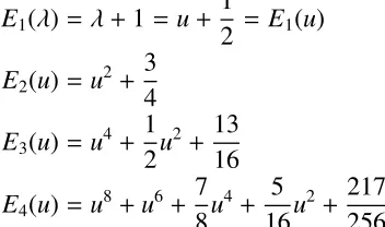
Expanding aboutλ = −1/₂ _{is clearly better than expanding about}λ = _{0. Put}_u = λ+1/₂_{, and}

then

E1(λ)= λ+1=u+

1

2 = E1(u)

E2(u)= u2+

3 4

E3(u)= u4+

1 2u

2₊ 13

16

E4(u)= u8+u6+

7 8u

4₊ 5

16u

2₊ 217

256

and these polynomials only have even powers (afterk= 1); this makes the polynomials subject to only half as much rounding error because zero coefficients cannot (are not allowed to) be perturbed. More, the coefficients of the even order terms appears to grow more slowly.

However, they do still grow doubly exponentially with k(exponentially with the degree). The first polynomial to have a coefficient larger than 1 in magnitude isE5(u)=u16+2u14+· · ·+

57073/₆₅₅₃₆_{and thereafter the repeated squaring gives runaway growth. We present the graphs of}

the condition numbers for the evaluation ofEk(λ)

e

Bk(u)=

deg(Ek) X

j=0

vj

|u|

(41)

(a) Pseudozeros of E6(λ) for 10 logarithmically-spaced values of ε be-tween 10−9.5and 10−8.5. The eigenvalues between −1.5 ≤ Re(λ) ≤ −0.5 is quite ill-conditioned. We only change E₆(λ) by 3×10−6% at most.

(b) Pseudozeros of E₆(u) for 10 logarithmically-spaced values of ε between 10−3 and 10−2. This is sub-stantially better-conditioned (and more symmetric) than the monomial basis (Figure 3.3a) changing Ek(λ) by 1% at most.

(c) Pseudospectra of E6 for 10 logarithmically-spaced values of ε between 10−2 and 10−1. This is the best-conditioned of the representations. This figure shows the results of changing

E6by 1–10%.