Shielding Effectiveness of Multiple-Shield Cables with Arbitrary
Terminations via Transmission Line Analysis
Salvatore Campione*, Lorena I. Basilio, Larry K. Warne, H. Gerald Hudson, and William L. Langston
Abstract—In this paper we report on a transmission-line model for calculating the shielding effectiveness of multiple-shield cables with arbitrary terminations. Since the shields are not perfect conductors and apertures in the shields permit external magnetic and electric fields to penetrate into the interior regions of the cable, we use this model to estimate the effects of the outer shield current and voltage (associated with the external excitation and boundary conditions associated with the external conductor) on the inner conductor current and voltage. It is commonly believed that increasing the number of shields of a cable will improve the shielding performance. However, this is not always the case, and a cable with multiple shields may perform similar to or in some cases worse than a cable with a single shield. We want to shed more light on these situations, which represent the main focus of this paper.
1. INTRODUCTION
Protecting a device from coupling of an external electromagnetic environment through a cable shield is at times a formidable task. Early work on solid shields can be found in Schelkunoff’s paper [1], and valuable information on cables and shielding can be found in various textbooks [2–5]. Shielding effectiveness is a common quantity that represents the shielding performance, measured as the reduction of the electromagnetic field at a given point in space (e.g., at a point in the inner conductor in the case of a cable) caused by placing a shield between the source and that point. Early works on shielding effectiveness of cables can be found in [6–8]. It is generally thought that increasing the number of shields of a cable will improve the shielding performance [9, 10]. However, there are situations in which a cable with multiple shields may perform similar to or worse than a cable with a single shield, and this has been seldom discussed in literature.
To address the question of shielding effectiveness in multiple-shield cables, we rigorously formulate a transmission-line model for determining the shielding effectiveness of such cables in the presence of arbitrary terminations. We assume the presence of an external excitation that produces the outer shield current and voltage which, in turn, induces the internal currents and voltages on the inner shield(s) and conductor. This non-zero transfer function results because the shields are not perfect conductors and apertures in the shields permit external magnetic and electric fields to penetrate into the interior region of the cable. We will analyze various cable configurations with varying numbers of shields and termination loads, whose shielding effectiveness will be compared. This cable survey will highlight the fact that cables with multiple shields may at times not exhibit much improvement relative to single-shield cables (and in certain frequency regions perform worse than single-single-shield cables), possibly not providing the extra protection desired.
Received 24 March 2016, Accepted 12 June 2016, Scheduled 25 June 2016 * Corresponding author: Salvatore Campione ([email protected]).
2. TRANSMISSION-LINE MODEL OF MULTIPLE-SHIELD CABLES WITH ARBITRARY TERMINATIONS
2.1. Case of a Single Shield
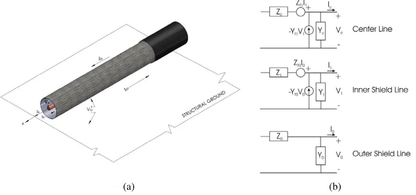
In order to model a shielded cable, we consider an element of transmission line of differential length dz that contains a distributed voltage source Ez(z) = ZTI0(z), where I0(z) is the current on the outer shield, as well as a distributed current source Jz(z) = −YTV0(z), where V0(z) is the external voltage on the outer shield. For reference, the external and internal electrical quantities for a shielded cable are labeled in Fig. 1(a). The shield properties (related to the braid weave characteristics and material) are accounted for in the per-unit length transfer impedance ZT and transfer admittanceYT.
More specifically, these terms capture the magnetic and electric field coupling mechanisms from the exterior of the cable to the inner conductor. For the purposes of this paper, it is assumed that these quantities are known (and determined from the particular braid characteristics [11–13]) and can be directly incorporated into the transmission-line model.
(a) (b)
Figure 1. (a) Voltages and currents associated with shielded cable analysis. (b) Approximate per-unit-length transmission line circuits for the double-shield cable case.
The differential equations for the voltage and current on the inner conductor of the braided cable (Vc andIc) are given by
dVc
dz +ZcIc =ZTI0(z) dIc
dz +YcVc =−YTV0(z). (1) In addition to the transfer parameters associated with the external cable characteristics, Eq. (1) also contains the per-unit length (series) self-impedance Zc and (shunt) self-admittance Yc, which are
formed by the inner conductor and the shield. As with the transfer impedance and transfer admittance, it will be assumed in this paper that the self-parameters characterizing the shielded cable geometry are known. From Eq. (1), it is clear that the sources for the transmission line are defined by the transfer parameters of the shielded cable and that these sources drive the coupled voltage and current on the inner conductor of the cable. At this point, we rewrite the second differential equation in Eq. (1) in a generalized form that allows for cases when the braided cable is located within an arbitrary structure such as a metallic cavity of arbitrary shape. In other words, we recognize that there may be situations where the exterior voltageV0(z) is not easily defined. Relating the transfer admittanceYT to the transfer
capacitance CT, we can write
dIc
dz +YcVc =−jωCTV0(z) =−jωCT q0(z)
C0 ,
whereq0(z) andC0 represent the charge and capacitance per-unit length of the outer shield, respectively. Since the transfer capacitance is proportional to the outer capacitanceC0, Eq. (2) can also be expressed as
dIc
dz +YcVc =−jωC˜Tq0(z), (3) where ˜CT is the transfer capacitance normalized by C0. Using the current continuity equation ∇ ·j =−jωρ0 or equivalently dIdz0 =−jωq0(z), Eq. (3) becomes
dIc
dz +YcVc = ˜CT dI0(z)
dz . (4)
Note that with the first differential equation in Eq. (1) and Eq. (4), the interior voltage and current can be found directly from the exterior cable currentI0(z) (and its derivative) and the transfer parameters characterizing the braided shield.
To solve the interior system of Eqs. (1) and (4), we will consider one source at a time and then apply a superposition of results for the final value of the inner conductor current [2]. Thus, assuming Jz(z) = ˜CTdIdz0(z) = 0 and using Eq. (1), the second-order differential equation for the inner conductor
current becomes
d2 dz2 −γ
2
c
Ic =−YcEz(z) =−YcZTI0(z), (5)
whereγc2=ZcYc. The solution of Eq. (5) is given by
Ic,e(z) = [K1,e+Pe(z)]e−γcz+ [K2,e+Qe(z)]eγcz
Vc,e(z) =
Zc
Yc
[K1,e+Pe(z)]e−γcz−[K2,e+Qe(z)]eγcz
, (6)
with Pe(z) = 12 Yc Zc z z−
eγczE
z(z)dz and Qe(z) = 12
Yc
Zc z+
z
e−γczE
z(z)dz, with Ez(z) = ZTI0(z). The
constants in Eq. (6) are determined from the terminating impedances ZL,c− and Z
+
L,c to the interior
transmission line (at locations z− and z+, respectively, wherez−< z < z+). More specifically,
K1,e=ρ−eγcz−ρ+Pe
(z+)e−γcz+−Qe(z−)eγcz+
eγc(z+−z−)−ρ
−ρ+e−γc(z+−z−)
K2,e=ρ+e−γcz+ρ−Qe
(z−)eγcz−−Pe(z+)e−γcz− eγc(z+−z−)−ρ
−ρ+e−γc(z+−z−) ,
(7)
where the reflection coefficients at positionsz− and z+ are ρ−=
ZL,c− −ZcYc
ZL,c− +ZcYc and ρ+=
ZL,c+ −ZcYc
ZL,c+ +ZcYc. With Eq. (6) accounting for the interior current driven by magnetic coupling and diffusion of the exterior field into the inner conductor, we now move on to accounting for the current contribution associated with the electric coupling of the exterior field. For this case, we assume Ez(z) = 0 so that
we obtain (where we have used the second differential equation in Eq. (12) withY0=jωC0)
d2 dz2 −γ
2
c
Vc =−ZcC˜TdI0
(z)
dz , (8)
and thus
Vc,j(z) = [K1,j+Pj(z)]e−γcz+ [K2,j+Qj(z)]eγcz
Ic,j(z) =
Yc
Zc
[K1,j+Pj(z)]e−γcz−[K2,j+Qj(z)]eγcz
withPj(z) = 12 Zc Yc z z−
eγczJ
z(z)dz and Qj(z) = 12 Zc Yc z+ z
e−γczJ
z(z)dz, withJz(z) =−YTV0(z), and
K1,j=ρ−eγcz−Qj
(z−)eγcz+ +ρ+Pj(z+)e−γcz+ eγc(z+−z−)−ρ
−ρ+e−γc(z+−z−)
K2,j=ρ+e−γcz+Pj
(z+)e−γcz−+ρ−Qj(z−)eγcz−
eγc(z+−z−)−ρ
−ρ+e−γc(z+−z−) .
(10)
Thus, to obtain the total current and voltage induced on the inner conductor we sum the two individual contributions:
Ic(z) =Ic,e(z) +Ic,j(z)
Vc(z) =Vc,e(z) +Vc,j(z).
(11)
2.2. Case of Multiple Shields
Cables with more than one shield can be analyzed by applying the transmission-line model shown in Sec. 2.1 to each shield to obtain the current in the next shield until all shields have been accounted for. Assuming N shields, the outer to inner shields to be indexed as 0, 1, 2, . . .,N−1, the differential equations for the voltage and current on the 0th shield (outermost shield) are given by
dV0
dz +Z0I0 =ZT,0I1, dI0
dz +Y0V0 =−YT,0V1. (12) In what follows, we neglect the interaction from the cable to the driving circuit using the weak coupling assumption, i.e.,ZT,0I1 = 0 and YT,0V1= 0. If the weak coupling assumption is not valid, the solution of the differential equations can be obtained although it is more complex. Thus, we assume that the current distribution on the outermost shield I0(z) is known.
The internal problem is now set by looking at theith internal shield, withi= 1,2, . . . , N−1, as
dVi
dz +ZiIi=ZT,(i−1)I(i−1)+ZT,iI(i+1) dIi
dz +YiVi= ˜CT,(i−1) dI(i−1)
dz + ˜CT,i dI(i+1)
dz
(13)
Again, we will neglect the interaction from the cable to the driving circuit, i.e., ZT,iI(i+1) = 0 and ˜
CT,i dI(i+1)
dz = 0. From Eq. (13), it is clear that the sources for theithtransmission line are defined by the
transfer parameters of the (i−1)th shield and that these sources drive the coupled voltage and current on the interior shield. We highlight this fact in Fig. 1(b) where we report approximate per-unit-length transmission line circuits for the double-shield cable case.
We will again consider one source at a time and then apply a superposition of results for the final value of the interior current. Eq. (6) can be used to computeIi,e(z) andVi,e(z) as a result of the interior
current driven by magnetic coupling and diffusion of the exterior field into the inner conductor, but now using the ith shield parameters and Ez(z) =ZT,(i−1)I(i−1). In a similar way, the required constants in Eq. (7) are now determined from the terminating impedancesZL,i− andZL,i+ to the interior transmission line (at locations z− andz+, respectively, wherez−< z < z+) using the ith shield parameters.
In a similar manner, Eq. (9) can be used to compute Ii,j(z) and Vi,j(z) as a result of the
current contribution associated with the electric coupling of the exterior field, but now using the ith shield parameters and Jz(z) = −YT,(i−1)V(i−1). Similarly, the required constants in Eq. (10) are now determined from the terminating impedances ZL,i− and Z
+
L,i to the interior transmission line using the
Finally, the differential equations for the voltage and current on the inner conductor of the braided cable (Vc andIc) are given by
dVc
dz +ZcIc =ZT,(N−1)I(N−1) dIc
dz +YcVc = ˜CT,(N−1)
dI(N−1) dz .
(14)
From Eq. (14), it is clear that the sources for the innermost transmission line formed by the (N −1)thshield and the inner conductor are defined by the transfer parameters of the (N −1)thshield and that these sources drive the coupled voltage and current on the inner conductor of the cable. See Fig. 1(b) where this is reported for the double-shield cable case.
We will again consider one source at a time and then apply a superposition of results for the final value of the inner conductor current. Eq. (6) can be used to computeIc,j(z) andVc,j(z) as a result of
magnetic coupling and diffusion of the exterior field into the inner conductor, but now using the inner conductor parameters andEz(z) =ZT,(N−1)I(N−1). In a similar way, the required constants in Eq. (7) are now determined from the terminating impedancesZL,c− andZ
+
L,cto the interior transmission line (at
locations z− and z+, respectively, where z−< z < z+) using the inner conductor parameters.
In a similar manner, Eq. (9) can be used to compute Ic,j(z) and Vc,j(z) as a result of the current
contribution associated with the electric coupling of the exterior field, but now using the inner conductor parameters and Jz(z) = −YT,(N−1)V(N−1). Similarly, the required constants in Eq. (10) are now determined from the terminating impedances ZL,c− and Z
+
L,c to the interior transmission line using
the inner conductor parameters. Thus, to obtain the total current and voltage induced on the inner conductor we sum the two individual contributions as done in Eq. (11).
3. NUMERICAL EXAMPLES
In this section, we will impose the distribution of the (outermost shield) disturbing current to be known and equal toI0(z) =I0e−γ0z. We will then estimate the shielding effectiveness as
SE(z) = 20 log10Ic(z) I0(z).
(15)
We would like to stress that the definition in Eq. (15) also complies with the definition of ratio of current in the core with and without the shield. In our particular drive condition we are not looking to the response to an incident wave, but to a forced current source. Therefore, if the shield is removed, our drive condition would inject a current on the core conductor of known value I0(z); then, if we put the shield on, our drive condition would impose a known current on the shield and we would find the current on the core conductor Ic(z). Then, we define shielding effectiveness as the ratio of the current
in the center conductor in the second case (with shield) to the one in the first case (no shield). This is exactly the definition of shielding effectiveness as the ratio of current in the core with and without the shield.
We will also adopt the complete semi-empirical model assembled by Kley [11] based on measurements of typical commercial cables. More accurate models could be adopted, e.g., multipoles [12, 13], but they are not necessary for the effects we are interested in in this paper. Unless otherwise stated, we will assume a PEC inner conductor and braid for the description of Zc and the
propagation impedances; this assumption is not applied to the transfer parameters.
3.1. Single Shield Cable Analysis and Experimental Verification
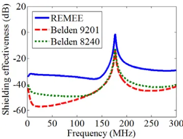
Figure 2. Shielding effectiveness for a 22-inch-long REMEE, Belden 9201, and Belden 8240 cable computed at z = −11 inch (the left termination end of the cable) assuming a load of 0.5 Ω at the inner conductor transmission line.
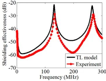
Figure 3. Comparison of measured and theoretical shielding effectiveness for a 22-inch-long Belden 8240 cable computed at the load side (atz=−11 inch).
Table 1. Simulation parameters for the load to model the experiment.
Frequency (MHz) 10 60 86 160 200 300
RL(Ω) 0.50 0.60 0.70 1.00 1.25 2.80
LL(nH) 25.7 25.7 25.7 27.0 28.0 32.0
accounts for the shield diffusion effect, withγ = 1−δj = (1.21−j1.21)×103 ω/ω0inch−1,δ=
2
ωμ0σ =
8.2×10⁻⁴ ω0/ωinch the skin depth, Rgs ={34.28,18.34, 13.34}mΩ/m, anddR={3.68,3.47, 3.5} ×
10−3inch for{REMEE,Belden 9201,Belden 8240},ZS= (1 +j)ωLS is the internal transfer impedance
assumed to be a forty five degree quantity, with LS = {821,−217.6,−462.6} ω0/ωpH/m for {REMEE,Belden 9201,Belden 8240}, YT = jωCT, with LT = {5614.6, −134.6, −754.9}pH/m and
CT ={863.07,177.9,7.3}fF/m for{REMEE,Belden 9201,Belden 8240}. We plot in Fig. 2 the shielding
effectiveness computed at z = −11 inch (a termination end) assuming a load of 0.5 Ω at both ends of the inner conductor transmission line for the three cables.
We observe a resonating behavior at around 175 MHz. A comparison of the three cables leads to the conclusion that the REMEE cable provides the lowest level of shielding, whereas the two Belden cables have comparable shielding effectiveness (with the Belden 9201 having slightly better performance at these frequencies). This result appears to be counterintuitive since the 8240 cable has a higher optical coverage leading one to believe that it should have better shielding performance. However, the shield topology of the Belden 9201 features near cancellation of the porpoising and hole effects [15], leading to better shielding effectiveness.
In order to provide confidence in our transmission-line model, we measure and report in Fig. 3 and Fig. 4 the shielding effectiveness of two 22-inch long Belden 8240 and Belden 9201 cables. In the experiment, we measure the current on the load as well as the current on the shield, with which we are able to determine the shielding effectiveness. To use the model described in Sec. 2, we should understand the experimental conditions. The current probes at the ends of the cable tester representZL→ 0.5 Ω
loads at low frequencies. Near the resonance of the tester it was found that the loads exhibit increasing losses as well as reactive effects. Thus, to get a better understanding of these load values, several experiments were performed [16]. The load ZL=RL+jωLLhas been approximated in simulation as a
Figure 4. Comparison of measured and theoretical shielding effectiveness for a 22-inch-long Belden 9201 cable computed at the load side (atz=−11 inch).
Figure 5. Shielding effectiveness for a 22-inch-long single and double-shield cable (referred to as SS and DS in the legend, respectively) computed at z = −11 inch assuming a load of 0.5 Ω at the inner conductor transmission line. The inner shield transmission line is considered to be shorted or matched.
Table 2. Simulation parameters for the cable attenuation to model the experiment.
Frequency (MHz) 1 10 50 100 200 400
Rc( ω/ω0Ω/m) Belden 8240 0.367 0.428 0.435 0.469 0.488 0.516 Rc( ω/ω0Ω/m) Belden 9201 0.496 0.471 0.509 0.523 0.527 0.564
been approximated in simulation as a linear interpolation function with the parameters in Table 2. For both cables analyzed, we find good agreement between experiments and theory, in both the level of the shielding effectiveness as well as the resonance frequency location.
It is our goal now to investigate if the use of multiple shields helps improve shielding effectiveness, and under what conditions. This is done in the next subsections in more detail.
3.2. Termination Effect and Losses Effect in Multiple-Shield Cables
Let’s focus our attention on the 22-inch-long commercial Belden 8240 cable analyzed in Fig. 2. We now analyze a double-shield cable, where we introduce a second shield with the same parameters as the shield of the Belden 8240 cable. The braid outer and inner diameters are 0.134 and 0.116 inches, respectively, and the wire diameter is 0.005 inches. We compute the shielding effectiveness atz=−11 inch assuming a load of 0.5 Ω at the inner conductor transmission line. Moreover, the inner shield transmission line is considered to be either shorted or matched. As shown in Fig. 5, when the inner shield transmission line is matched, the shielding effectiveness of such a double-shield cable is better than the single-shield cable in the entire frequency range analyzed. However, when it is shorted, an additional resonance around 260 MHz appears, where the cable behaves much worse than the single-shield cable. We believe that this resonance arises from the fact that the inter-shield region is a shorted transmission line of finite length, and the resonance is dictated by the permittivity of the dielectric between shields and the parameters of the shields. This is an important result to be taken into account for proper shielding engineering.
The cable attenuation is important to include at the resonances. We will include the cable attenuation by inserting center conductor losses Rc = 0.43 ω/ω0 inZc [14], with ω0 = 2π×107rad/s. We thus repeat the investigation of Fig. 5 including center conductor losses, and report the result in Fig. 6. It can be observed that the inclusion ofRc reduces the level of shielding effectiveness at 175 MHz
Figure 6. The shorted DS case in Fig. 5, but now considering center conductor losses Rc =
0.43 ω/ω0.
Figure 7. The shorted DS case in Fig. 5, but now considering the shield loss resistance.
Let’s now take into account that the shields may have a non-negligible resistive component. We include the shield loss resistance and show the result in Fig. 7. We observe that now, in contrast to the center conductor losses, only the extra resonance at 260 MHz is affected by shield loss. This resistive component dampens the resonance at 260 MHz, limiting its quality factor. Even in this case, however, the double-shield cable has worse shielding effectiveness around 260 MHz than the single-shield version shown in Fig. 5. Note that without the shield losses (in this approximate model) the level of the 260 MHz resonance is not finite.
3.3. Sizing Effect in Double-Shield Cables
Here we show that the geometry of the shields can greatly affect the shielding effectiveness of double-shield cables. In particular, we modify the innerb1and outerb0radii of the braid (and necessarily change the distance between the shield conductors, and thereby their inductive and capacitive coupling) and plot the shielding effectiveness in Fig. 8 compared to the single-shield case. When the two shields are very close to each other, i.e.,b0/b1∼= 1, one can see that the cable behaves the same (the region below
Figure 8. Shielding effectiveness for a 22-inch-long single- and double-shield cable computed at z=−11 inch assuming a load of 0.5 Ω at the inner conductor transmission line. The inner shield transmission line is considered to be shorted. Shield radii dimensions are modified as detailed in the legend, which shows the ratio b0/b1.
150 MHz) or worse than the single-shield one (the resonance region). Thus, little or no improvement is obtained by adding a second shield. Proper design and modeling is thus necessary to understand the proper effectiveness of shields, especially for applications where shielding is of vital importance. Increasing the distance between the shields leads to an overall improvement of the shielding effectiveness by more than 20 dB. Also in this case, however, the double-shield cable behaves worse than a single-shield one at 260 MHz.
We then modify the dielectric permittivity between the two shields to a value of 1.67, and replot in Fig. 9 the result observed in Fig. 8. As expected, this affects mostly the extra resonance at 260 MHz (due to the short circuit at the inner-shield transmission line) which is now moved to 210 MHz upon increase in dielectric contrast between the two shields.
4. CONCLUSION
In this paper we formulated a transmission-line model for calculating the shielding effectiveness of multiple-shield cables with arbitrary terminations. We have shown, with multiple examples, that increasing the number of shields of a cable may not improve the shielding performance. In particular, we observed that the shielding terminations are one of the main parameters to account for when designing shields.
ACKNOWLEDGMENT
We acknowledge T. L. Smith, Sandia National Laboratories, for the construction of Fig. 1(a). This work was supported in part by Sandia Corporation, a wholly owned subsidiary of Lockheed Martin Corporation, for the U.S. Department of Energy’s National Nuclear Security Administration under contract DE-AC04-94AL85000.
REFERENCES
1. Schelkunoff, S. A., “The electromagnetic theory of coaxial transmission lines and cylindrical shields,”Bell System Technical Journal, Vol. 13, 532–579, 1934.
2. Vance, E. F., Coupling to Shielded Cables, R. E. Krieger, 1987.
3. Lee, K. S. H., EMP Interaction: Principles, Techniques, and Reference Data, Hemisphere Publishing Corp., Washington, 1986.
4. Celozzi, S., R. Araneo, and G. Lovat, Electromagnetic shielding, John Wiley and Sons, 2008. 5. Tesche, F. M., M. V. Ianoz, and T. Karlsson, EMC Analysis Methods and Computational Models,
John Wiley & Sons, Inc., New York, 1997.
6. Vance, E. F., “Shielding effectiveness of braided wire shields,”Interaction Note 172, 1974.
7. Knowles, E. D. and L. E. Olson, “Cable shielding effectiveness testing,” IEEE Transactions on Electromagnetic Compatibility, Vol. 16, 16–23, 1974.
8. Schulz, R. B., V. C. Plantz, and D. R. Brush, “Shielding theory and practice,” IEEE Transactions on Electromagnetic Compatibility, Vol. 30, 187–201, 1988.
9. Jayasree, P. V. Y., V. S. S. N. S. Baba, B. Prabhakar Rao, and P. Lakshman, “Analysis of shielding effectiveness of single, double and laminated shields for oblique incidence of EM waves,” Progress In Electromagnetics Research B, Vol. 22, 187–202, 2010.
10. Demoulin, B., P. Degauque, M. Cauterman, and R. Gabillard, “Shielding performance of triply shielded coaxial cables,” IEEE Transactions on Electromagnetic Compatibility, Vol. 22, 173–180, 1980.
11. Kley, T., “Optimized single-braided cable shields,” IEEE Transactions on Electromagnetic Compatibility, Vol. 35, 1–9, 1993.
13. Warne, L. K., W. L. Langston, L. I. Basilio, and W. A. Johnson, “First principles cable braid electromagnetic penetration model,” Progress In Electromagnetics Research B, Vol. 66, 63–89, 2016.
14. Hudson, H. G., S. L. Stronach, W. Derr, W. A. Johnson, L. K. Warne, J. Kotulski, et al., “Cable test system upgrade coaxial cable/connector model validation experiments,” Facility Test Report, Albuquerque, NM, 2001.
15. Tyni, M., “The transfer impedance of coaxial cables with braided outer conductor,” FV. Nauk, 410–419, Inst. Telekomum Akust. Politech Wroclaw, Ser. Konfi, 1975.