Finding Nonlinear Relationships in Functional Magnetic Resonance Imaging Data with Genetic Programming

(1)

Western University Western University

Scholarship@Western

Electronic Thesis and Dissertation Repository

7-10-2018 10:00 AM

Finding Nonlinear Relationships in Functional Magnetic

Resonance Imaging Data with Genetic Programming

James Hughes

The University of Western Ontario

Supervisor Mark Daley

The University of Western Ontario

Graduate Program in Computer Science

A thesis submitted in partial fulfillment of the requirements for the degree in Doctor of Philosophy

Follow this and additional works at: https://ir.lib.uwo.ca/etd

Part of the Artificial Intelligence and Robotics Commons, and the Computational Neuroscience Commons

Recommended Citation Recommended Citation

Hughes, James, "Finding Nonlinear Relationships in Functional Magnetic Resonance Imaging Data with Genetic Programming" (2018). Electronic Thesis and Dissertation Repository. 5491.

https://ir.lib.uwo.ca/etd/5491

This Dissertation/Thesis is brought to you for free and open access by Scholarship@Western. It has been accepted for inclusion in Electronic Thesis and Dissertation Repository by an authorized administrator of

(2)

The human brain is a complex, nonlinear dynamic chaotic system that is poorly understood. When faced with these difficult to understand systems, it is common to observe the system and develop models such that the underlying system might be deciphered. When observing neurological activity within the brain with functional magnetic resonance imaging (fMRI), it is common to develop linear models of functional connectivity; however, these models are incapable of describing the nonlinearities we know to exist within the system.

A genetic programming (GP) system was developed to perform symbolic regression on recorded fMRI data. Symbolic regression makes fewer assumptions than traditional linear tools and can describe nonlinearities within the system. Although GP is a powerful form of machine learning that has many drawbacks (computational cost, overfitting, stochastic), it may provide new insights into the underlying system being studied.

The contents of this thesis are presented in an integrated article format. For all articles, data from the Human Connectome Project were used.

In the first article, nonlinear models for 507 subjects performing a motor task were created. These nonlinear models generated by GP contained fewer ROI than what would be found with traditional, linear tools. It was found that the generated nonlinear models would not fit the data as well as the linear models; however, when compared to linear models containing a similar number of ROI, the nonlinear models performed better.

Ten subjects performing 7 tasks were studied in article two. After improvements to the GP system, the generated nonlinear models outperformed the linear models in many cases and were never significantly worse than the linear models.

Forty subjects performing 7 tasks were studied in article three. Newly generated nonlinear models were applied to unseen data from the same subject performing the same task (intra-subject generalization) and many nonlinear models generalized to unseen data better than the linear models. The nonlinear models were applied to unseen data from other subjects perform-ing the same task (intersubject generalization) and were not capable of generalizperform-ing as well as the linear.

Keywords: Functional Magnetic Resonance Imaging, Nonlinear Relationships, Functional Connectivity, Symbolic Regression, Genetic Programming, Timeseries

(3)

Co-Authorship Statement

I would like to acknowledge Mark Daley, my supervisor as a coauthor on the integrated articles. James Hughes wrote the genetic programming system, designed the experiments, executed the experiments, analyzed the results, and wrote the articles.

(4)

First, I would like to thank Mark Daley, my supervisor, for his leadership and support throughout this journey. His careful and meticulously well-crafted advice and guidance was fundamentally necessary for my success in both my graduate work, and in life.

I would like to thank Ethan Jackson, whom I have been studying computer science with for many years. Not only has his support helped me through my PhD, but also my Masters and Undergraduate degree. I’m not entirely sure I would have gotten through third year algorithms without our long study sessions in MC D205.

I would also like to thank the current and past members of the lab. I’ve always enjoyed talking about the research and sharing ideas. On multiple occasions, many critical ideas were brought up that greatly improved my work.

I thank the people within the Computer Science department here at the University of West-ern Ontario. Whether a student, teacher, peer, or administrator, many have played a large role throughout the past 4 years. I really do feel that I have grown a lot during this time, and it was those within my direct community that had the greatest impact.

Additionally, I thank those within the computer science department at Brock University, where I completed my Undergraduate and Masters degrees. It was the faculty members and friends I made there that sparked my excitement for computer science.

I would like to thank my family. Not only have they supported me throughout my studies, they have enabled me to be where I am today. They enabled me to enroll in a PhD, Masters, and Undergraduate degree. They supported me throughout high school. They instilled upon me my work ethic and curiosity. Ultimately, they made me into who I am today.

Above all, I thank Matea Drljepan. We have been pushing and supporting each other for the sake of our future together since 2008. Whether it was specific edit suggestions, or higher-level motivation, she has always patiently helped.

(5)

List of Figures

1.1 A snapshot of a brain when segmented into the 30 ROIs as seen in FSL view. Each colour represents a different region. . . 3

2.1 Example, high level description of a typical evolutionary algorithm. . . 9 2.2 One point crossover example with a simple binary value representation. All

values within the darker emphasised area are swapped between the two chro-mosomes. This figure also shows a simple binary representation. . . 11 2.3 In this example, each circle represents a separate population (4 in this case)

which evolve independently from one another. After some number of genera-tions, chromosomes from each population have the opportunity tomigrateto other populations. This particular figure shows allowable migrations between all populations, however this is not a requirement. . . 12 2.4 Three exampleprogramsrepresented in a tree-structure. . . 13 2.5 Example of a one point crossover operation between two tree-structure

chro-mosomes. . . 14 2.6 Figures 2.6a and 2.6b both represent the same expression: (1.23−x)+sin((1.23−

x)·y·ex). Figure 2.6c shows a possible encoding for an acyclic graph with an array. . . 16 2.7 High level overview of a GP system implementation with fitness predictors

evolving in parallel. This particular example contains multiple sub-populations. 17

3.1 Hemodynamic Response Function [15]. After an event/neural spike, the rela-tive deoxygenated blood levels increases (sometimes with an initial dip before the increase) and after roughly 10 seconds, levels returns to close to baseline. . 20

Article 1.1: A snapshot of a brain when segmented into the 30 ROIs. Each colour represents a different region. . . 28 Article 1.2: Figures 2a and 2b both represent the same expression: (1.23−R10)+

S in((1.23−R10)∗R30∗eR10), however, Figure 2b was able to represent the same information as Figure 2a with less resources. In this example,bluenodes represent binary operators,rednodes represent unary operators, andgreynodes represent a terminals;Rxsignifies a variable (region of interest in this case) and a number signifies a constant. . . 29 Article 1.3: High level structure of this symbolic regression implementation. The left

side demonstrates the evolution of the expressions while the right side depicts the evolution of fitness predictors. This example shows only three subpopula-tions evolving in parallel. . . 29

(8)

lines represent nonlinear and linear relationships, and black lines represent strictly linear relationships. This particular example corresponds to the equa-tion:R21=R12−sin(11.97∗(18.30−R12))−(0.42∗ |(R12−R18)∗R27|)/(R6−

tan(R2)) which had a absolute average error from the measured signal of 12.4. . 30 Article 1.5: Time series of ROI 21’s signal compared to the generated nonlinear and

linear models. It is clearly depicted that both models can fit the data very well over the whole time series. An interesting observation is that the models are closer to one another than to the recorded signal. . . 32

Article 1.6: ROI count averaged and compared to False Discovery Rate with 95%. Almost all ROIs are always related to ROI 21 with this popular neuroimaging thresholding technique. . . 32

Article 1.7: ROI count averaged and compared to top 3 of the False Discovery Rate with 95%. Note that the average number of ROI that appeared in a nonlinear model over all models on all subjects is slightly less than 3 (4 when counting ROI 21). Because of this, the comparison with the top 3 ROI (4 when counting ROI 21) in the linear model will not exactly match. . . 32

Article 2.1: Siemens 3T Magnetom Prisma functional Magnetic Resonance Imaging scanner located in the Robarts Research Institute at the University of Western Ontario. . . 36

Article 2.2: A snapshot of a brain when segmented into the 30 ROIs. Each color represents a different region. . . 37

Article 2.3: An array encoding for the expressions (1.23−x)+S in((1.23−x)∗y∗ex). Sub-expressions can be referenced multiple times by any number of operators in a higher index. ‘?’ represent information not expressed in the phenotype, however they may containvestigialsub-expressions [102]. . . 38 Article 2.4: High level structure of this symbolic regression implementation. The left

side demonstrates the evolution of the expressions while the right side depicts the evolution of fitness predictors. This example shows only three subpopula-tions evolving in parallel. . . 38

Article 2.5: Probability value transition plot between the linear and nonlinear mod-els’ mean absolute errors (averaged over all subjects per task) as the number of the top linearly correlated ROIs used to fit the data with linear regression is increased. The number of ROIs used in the nonlinear models was fixed as the number of ROIs linear models used were increased. . . 40

Article 2.6: Nonlinear and Linear models expected ROI intensity value compared to the measures signal. . . 40

Article 2.7: Representations of where the linear and nonlinear models disagree on what ROIs are important in describing the system. . . 41

(9)

Article 2.8: From left to right, the best mean absolute error values averaged over all subjects when performing the same task for nonlinear models, linear models generated with false discovery rate, and linear models generated with all ROIs respectively. For example, row M and column L contains the averaged mean absolute error values of the models for all subjects fit to the language task, but applied to the motor task’s data. . . 42

Article 3.1: A three-dimensional snapshot of the four-dimensional fMRI data. The voxels in this brain contain the BOLD signal from a single time point. . . 45 Article 3.2: p-value transition plot comparing linear and nonlinear models’ mean

absolute errors (averaged over all subject) as the number of ROIs used to create the linear model increases. ROIs were added to the linear models in the order of their absolute correlation score. The number of ROIs in the nonlinear models was fixed. . . 47 Article 3.3: Number of subjects for each ROI (column) that appeared in the top

model for each task (row). Counts for the nonlinear and LASSO generated linear models are presented. The other liner models were excluded as they typically contained nearly all (or all) ROIs. 40 is maximum. Note that the ROI corresponding to the left hand side of the equation was in all models. . . 47 Article 3.4: Matrices showing the mean absolute error values obtained by applying

every task/subject combination’s models to all other datasets and averaged over all subjects performing the same task. The diagonal provides a means of quan-tifying intersubject generalization; if all subject’s models on the same task can fit all other subject’s data from that task similarly well, then the models are capable of generalizing between subjects. . . 49 Article 3.5: Scatterplot comparing the training and testing mean absolute errors for

all models. For the nonlinear model, the top model on the training data was compared to it’s error when applied to unseen data. . . 49 Article 3.6: Distribution of mean absolute error values when applying all 100

non-linear models to unseen data from the same subject performing the same task. Vertical lines correspond to the mean absolute errors obtained by linear models. 48 Article 3.7: Scatterplot comparing the smallest mean absolute error from the 100

nonlinear models when applied to unseen data versus the best of the 6 linear models. Points above they= xline indicate that the nonlinear model was best. Points below indicate that a linear model was best. Color indicates method for model generation. . . 49 Article 3.8: For each subject, the number of the 100 nonlinear models generated that

were better than the best linear model when applied to unseen data was cal-culated and the distributions were plotted. Bins (x-axis) represent the number of nonlinear models better than the best linear. The bin height (y-axis) corre-sponds to the number of subjects. . . 49 Article 3.9: Similar to Figure 4 (of the article), this matrix shows the mean absolute

error values obtained by applyingthe best model on the unseen datafrom every subject/task to all other datasets and averaged over all subjects performing the same task. . . 50

(10)

task. Note that the ROI corresponding to the left hand side of the equation was in all models. . . 51

B.1 Gamma function and approximation of the gamma function where−3< x< 3. Blue is the gamma function, the green points are the (x,Γ(x)) pairs provided to the GP system, and red is the model derived by the GP system. . . 71

(11)

List of Tables

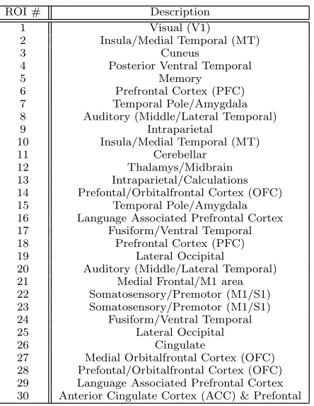
3.1 Data excerpt from subject 100307 performing the Emotion task after z-score normalization. This table demonstrates the tabular representation of the fMRI timeseries data. ROIs 6 through 29, and time points 10 through 175 were ex-cluded to conserve space. . . 23 3.2 Region of interest number and corresponding neuroanatomical region. This

table provides a frame for the resolution of the brain segmentation. . . 24

Article 1.1: Neroanatomical regions and their corresponding segmented regions of interest. This list provides a frame for the resolution of the currently attempt to model functional activity with symbolic regression. . . 28

Article 2.1: Neroanatomical regions and their corresponding segmented regions of interest. This list provides a frame for the resolution of the segmentation of the brain. . . 37 Article 2.2: summary of the top nonlinear models and linear models with different

correction for multiple comparison and thresholding techniques. MAE is the averaged mean absolute error over all subjects for each task and the proba-bility value (p-val.) was calculated with a Mann-Whitney U test between the nonlinear models and the respective column’s linear model. . . 40

Article 3.1: Region of interest number and corresponding neuroanatomical region. This table provides a frame for the resolution of the brain segmentation. . . 45 Article 3.2: Parameter settings for GP System. The last 4 settings are specific to the

improvements discussed in 4.1 (of the article). . . 46 Article 3.3: Summary statistics (median and in interquartile range (IQR)) for all

generated models along with probability values obtained with a Mann-Whitney U test when comparing the mean absolute errors of the nonlinear models to the respective linear model. . . 48 Article 3.3: Average difference between the best nonlinear and linear models’ mean

absolute errors when the respective column’s model was best. The values are averaged over all subjects performing the same task. Ex: for the emotion task, when nonlinear models were better than linear, they were on average better by 0.041. . . 50

B.1 Total CPU usage in core years for the project over a 4 year period. All project GP system executions were done on Compute Canada resources. . . 73

(12)

Appendix A: Published Works for Paper 1 70

Appendix B: Genetic Programming System Details 74

(13)

Chapter 1 Introduction

The human brain is a nonlinear computational system. Although neuroscience literature ex-plicitly acknowledges this [15, 18, 26, 38, 36, 122], it is commonly deemphasized or ignored, especially when working with functional magnetic resonance imaging (fMRI) data [18, 84]. When studying fMRI timeseries data to findfunctional relationshipswithin the brain, it is com-mon to exclusively use linear tools, such as Pearson product-moment correlation coefficient or the general linear model (GLM). However, these methods are not capable of describing what we know to be a nonlinear system as it lacks the power to truly model the underlying processes. In spite of this inability to truly model the system, neuroscientific studies make meaningful contributions to the field with these linear methods [18]. However, one must wonder if a more expressive, nonlinear method capable of describing the underlying system would increase the analytical power and significance of results. It is in no way surprising that the nonlinear relationships are ignored and more complex tools are not used since it is exceptionally difficult to find nonlinear relationships, especially when working with large amounts of noisy high-dimensional data from a nonlinear, dynamic complex system.

1.1 fMRI Data

Magnetic resonance imaging (MRI) scanners harness magnetic fields and electromagnetic en-ergy in a controlled way to capture localized information about physical properties of tissue within the brain1. More precisely, they capture information about thespin-relaxation proper-ties of particles within the brain (this idea is discussed further in Chapter 3). MRI scanners capture the localized information which can then be represented in the form of voxels — three-dimensional analogues to two-dimensional pixels. Ultimately, the whole brain can be represented as a three-dimensional structure made up of voxels to give a static view of the underlying three-dimensional anatomy.

Functional MRI records theblood oxygen level dependent(BOLD) signal — a measure-ment of the relative oxygenation level of blood within tissue — which is used as a proxy for brain activation. These relative blood oxygen level variations occur since neurons do not store their own energy, and after activation, the vascular system must replenish the resources to the cerebral tissue. This process is called thehemodynamic response(HDR) and is a consequence

1_{MRI technology is not restricted to brain imaging, however neuroimaging is the focus of this thesis.}

(14)

of metabolism. Although the BOLD signal is not actually brain activation, it can be used as a proxy and has been shown to strongly correlate with localized neural activity [95, 85, 84, 51].

The fMRI technology still captures images of the three-dimensional structure, however the information within the voxels is the BOLD signal.

Unlike MRI, which captures the three-dimensional anatomical information, fMRI captures the spatially localized BOLD signal from the three-dimensional brain. Since the moment-to-moment changes in neural activity are of interest, the scanner will take many three-dimensional snapshots of the brain over time such that the changes in the BOLD signal can be observed. The data being recorded is four-dimensional — the three-dimensional physical brain, over time (the additional dimension).

Often, subjects will be placed within an fMRI scanner and will be given some task, such as viewing images, playing a game, or moving a body part. By time-locking the task onsets with the observed BOLD signal, researchers try to determine which areas of the brain (voxels, or perhaps larger regions of interest (ROI)) are functionally related to the task being performed. This usage is sometimes calledtask-basedfMRI analysis.

Sometimes subjects are placed within a scanner and are instructed to perform no task at all. In this scenario, the idea is to observe the spontaneous changes in the BOLD signal during rest instead of comparing the signal to what is expected to be seen when some task is being performed. This approach is calledresting-statefMRI.

1.1.1 Graph Interpretation

Resting-state fMRI data is commonly used to develop functional connectivity models of the brain: if the BOLD signal within two areas of the brain (voxels, or ROI) appear to be moving together similarly in time, then they are said to be functionally connected. There are many ways one could measure area similarity over time, but the Pearson correlation coefficient is typically used to infer the functional connections (although in reality, all that can be said is that the two areas are linearly correlated).

By doing this, we can create a simple graph representation of the complex four-dimensional object. A simple graph is a collection of vertices/nodes connected together by edges. A vertex represents some entity, and an edge between two vertices represents some relationship between the entities. In this case, we treat the areas of the brain as vertices, and connect the vertices with an edge if the linear correlation score is above some predefined threshold. In this example, Pearson correlation was used to infer connectivities, however this is by no means a requirement. These graphs provide static views of the synchronization of areas of the brain and greatly simplify the four-dimensional data. These models enable researchers to study the data in new ways; there are many well-defined graph theory metrics that are now available to the researchers [113]. For example, the topology of the graph can be analysed to study clinical questions, like if there are topological differences/similarities between individuals with certain neurological disorders [88, 17], or between adult and adolescent brain networks [31].

1.1.2 Human Connectome Project Data

(15)

1.2. NeuroscientificMotivation 3

Figure 1.1: A snapshot of a brain when segmented into the 30 ROIs as seen in FSL view. Each colour represents a different region.

HDR.

The data selected for this analysis was obtained from the Human Connectome Project,

WU-Minn Consortium, which can be found athttp://www.humanconnectome.org/. The

Hu-man Connectome Project has an open database of a large collection of neuroimaging data, and as of April 2018, the database contains structural MRI, resting-state fMRI, diffusion imaging, and task-based fMRI data for roughly 1200 subjects, and Magnetoencephalography (MEG) data for resting-state and tasks on a subset of the participants.

The task-based fMRI data available from the Human Connectome Project include: Emo-tion, Gambling, Language, Motor, Relational, Social, and Working Memory. The actual tasks and number of subjects used varied throughout the project.

The fMRI timeseries data was segmented into meaningful ROIs (refer to Figure 1.1) with Craddock et al.’s spatially constrained parcellation[24]. Each voxel’s activation within each ROI was averaged to determine the ROI’s mean activation.

Although the fMRI timeseries data is a four-dimensional object (three-dimensional snap-shots of a brain over time), it can easily be represented as a two-dimensional matrix of voxels over time if the three-dimensional physical space of the brain is flattened into one long vector, and time is left as the other dimension. Each entry in the matrix corresponds to the BOLD sig-nal of a single voxel at a particular time point. Ultimately, the data can cleanly be represented in tabular format.

1.2 Neuroscientific Motivation

(16)

itself to discover properties about the complex system. For example, if we are interested in which regions of the brain are functionally connected, we may record resting-state or task-based fMRI data, fit a mathematical model to the data, and from the model determine which regions of the brain are related to one another, and in which way.

Typically the graphical models of functional connections are generated from resting-state fMRI data, however task-based fMRI data can also be used. By doing so, we can develop these functional connectivity models of the brain during certain tasks. Additionally, there is no need to restrict the model development to linear correlations.

For example, if we are interested in developing a model of functional connectivity, then we may perform some thresholding on the recorded data, and then develop a linear model of the data with the GLM. There are a couple of ways this could be done depending on the question being asked.

If we wanted to know how a given ROI X is functionally connected to all other ROIs, then we would calculate the Pearson product-moment correlation coefficients between the ROIs, perform some correction for multiple comparisons (typically false discovery rate (FDR) or

Bonferroni correction (BC)), and remove statistically unrelated ROIs. Finally, the remaining ROIs are regressed to our ROI X and the beta weights (coefficients) can be used to indicate relatedness during the task.

This, along with the simpler linear correlation strategy described above, assumes that the system is linear, however we know that the human brain is a nonlinear system. This strategy makes many additional assumptions, including: the ROIs are fixed values as opposed to random variables, constant variance in the data, and the errors are independent.

Statistically unrelated ROIs are eliminated with thresholding to ensure that only meaning-ful ROIs are included in the resulting model; however, what does it mean for an ROI to be meaningfully related? The brain is a connected system being recorded at the same time under the same circumstances, and unsurprisingly many ROIs end up being highly correlated. After thresholding, a large number of ROIs will typically be left asmeaningful— sometimes even all. Perhaps the whole brain is involved in the function of the task be studied, but this would seem unlikely.

Despite the assumptions described above, there are many reasons to prefer the traditional, simpler linear tools. Linear models are easy to generate, the tool is well understood, and the models are easy to interpret. More complex methodologies are susceptible to overfitting, the methods are harder to understand, the resulting models are difficult to interpret, and they typically have a much greater computational cost. However, despite these drawbacks, using a more complex method actually capable of describing the underlying nonlinear system may allow us to eliminate assumptions and develop a more accurate and descriptive model of the functional connectivities within brain.

1.3 Methods

(17)

1.4. NonlinearAnalysis of fMRIdata 5

to learn how to solve a given problem [69]. GP is used in this work to automate the process of finding minimal and interpretable network relationships in a system for which we can only observe a recorded timeseries from the system’s network’s nodes. Namely, GP is used to find nonlinear functional relationships within fMRI timeseries data with symbolic regression.

Symbolic regression is a type of regression analysis that, in addition to parameter optimiza-tion, searches for model structure by performing feature selection and exploring the space of mathematical expressions. A GP system was developed for this work that was specifically de-signed for symbolic regression. The GP implementation was based on Schmidt et al.’s work, and incorporates improvements to increase performance [106]. Noteworthy improvements in-clude a distributed population/island model, an acyclic graph representation [102], and fitness predictors [104, 105]. A summary of the method’s improvements is provided here, but more details on evolutionary computation and GP can be found in Chapter 2.

Typical GP systems employ a tree based representation [76], however many popular non-tree based representations exist. In this work, an acyclic graph representationis used. The implemented representation has a lightweight array based encoding that avoids bloat, scales well, and can reuse subexpressions [102].

Computational costs of the evolutionary search is greatly reduced with the use of fitness predictors, which approximates the local search gradient [104, 105]. The high level idea is to evaluate each candidate solution on a small, but representative subset of the data being fit to. The subset of data is always changing such that it contains data points the current candidate solutions do not fit well; it focuses the search on areas of the space that need the most improvement. Fitness predictors were shown to lower computational cost, reduces overfitting, and improves results [105].

For much of the work, symbolic regression was used to develop nonlinear models of the brain, which can be interpreted as graph/network models of nonlinear functional relationships. This nonlinear regression is capable of describing the actual nonlinearities that must exist within the underlying system; nonlinear regression is strictly more powerful than linear regres-sion in its descriptive power. Symbolic regresregres-sion also performs feature selection, eliminating the need to manually perform thresholding.

These nonlinear models were compared to linear models developed with typical methods employed within the neuroscientific literature (GLM and the Pearson product-moment coeffi -cient). A description of the methods used to develop the linear models are discussed within the integrated articles found in Chapters 4, 5, and 6. Each of the integrated articles found in Chapters 4, 5, and 6 also provide a description of the GP system and a summary of the sys-tem settings used for each project. Appendix B includes technical details about the GP syssys-tem implemented (version number, number of classes, lines of code).

1.4 Nonlinear Analysis of fMRI data

(18)

connectivities between neuronal regions of the brain [35]. Zhang et al. used a semi-parametric model built around Volterra series to characterize BOLD signal and found deviations from the linear models and showed that their approach outperformed many existing methods [126].

Symbolic regression, a type of regression analysis, was used to describe nonlinear functional connectivities between known networks inresting-state fMRI data [2]. These works are dis-cussed in more detail in Chapter 3.

The symbolic regression work done by Allgaier et al. in [2] is the most relevant to the work in this thesis as it also develops network models from nonlinear relationships found within fMRI data. Their work used resting-state data and focused on areas of the brain already known to exist within functional networks of interest. The work in this thesis searches for nonlinear re-lationships within task-based fMRI data within ROI throughout the whole brain. Additionally, the work contained within this thesis evaluates the models in different ways.

1.5 Contribution

A GP system incorporating a number of modular improvements was implemented and made publicly available. This GP system was developed for the purpose of finding nonlinear func-tional connectivities within fMRI data, however it is a specialized system for symbolic re-gression in general. Given the high dimensionality of the search space, the improvements incorporated into the system were required in order for the evolutionary search to complete in a reasonable amount of time. After the initial development of the system, numerous revi-sions were done over the past three years. Development of the GP system will continue for the foreseeable future.

While working within the limitations of the real task-based fMRI data available, a graph-based interpretation of the timeseries data was developed. Functional connectivities were mod-elled with a GP system specifically created for this project. These graph-based models of non-linear relationships were found to be much more succinct (fewer relationships) when compared to models developed with conventional linear tools.

This thesis demonstrates a methodology that will enable the longer term goal of finding meaningful nonlinear functional relationships within fMRI data, interpreting the meaning of these relationships, and making contributions to the neuroscientific literature.

Three articles are presented in this work and are the natural progression of the project. The first article presents the proof of concept by applying the GP system to data from a single task and exploring the differences between nonlinear and linear models of a network interpretation of fMRI data. In this article, data from 507 subjects were studied. It found the nonlinear models to contain fewer ROI than the linear models developed with typical linear methods, and the nonlinear models’ ROIs were almost always subsets of the linear models’ ROIs. It also found that the GP generated nonlinear models were not capable of fitting the recorded fMRI signal as well as the linear models.

(19)

1.6. ThesisFormat 7

now able to fit their data better than the linear models. There were many similarities in ROIs found between the model types, but the nonlinear models contained functional connectivities not found with linear tools.

The third article incorporates more subjects and a deeper analysis into the generalizability of the models to unseen data. In this article, data from 40 subjects were studied. Again, after improvements, the nonlinear models, on average, grew in size by a small amount over the previous work’s nonlinear models, but still contained fewer ROI than the linear models. However, LASSO regression was included in the comparison and the linear models created with LASSO regularization were of comparable size to the nonlinear. The nonlinear models fit their data better than the linear models, and their intersubject and intrasubject generalizability was explored to determine if the nonlinear models were effective, and not overfitting.

Ultimately, the nonlinear models fit data better than traditional linear models, and were ca-pable of generalizing to unseen data; however, the author very explicitly and clearly acknowl-edges the statistical biases and limitations of the current conclusions in Chapter 7. Methods for overcoming the limitations are discussed in Section 7.3 where future directions are presented.

1.6 Thesis Format

This thesis is presented in theintegrated-articleformat. Chapter 2 provides a background and literature review on evolutionary computation and GP. Chapter 3 provides background and a brief literature review for the fMRI data and related neuroscientific works. Chapters 4, 5, and 6 are integrated articles from works completed during the duration of the author’s PhD and are the natural progression of the overall project. Each of these chapters provide motivation, a small literature review, descriptions of the data used, and GP system implementation and settings details. Chapter 7 provides a discussion and concludes the work and includes possible future directions.

(20)

Evolutionary Computation and Literature

Review

This chapter provides background information forevolutionary computation(EC),genetic al-gorithms(GA), and GP, along with a brief literature review of some algorithmic enhancements. This chapter is derived from the Topics Survey/Proposalwritten in December 2015 and pre-sented June 2017. Brief details on the current implementation of the GP system can be found in Appendix B.

2.1 Genetic Algorithms

Evolutionary algorithms (EAs), a subcategory of evolutionary computation, are a population basedmetaheuristic— a high level algorithm designed to guide a problem space exploration — which search by simulating the process of biological evolution through a series of nature inspired operations: mutations, sexual reproduction, recombination, and natural selection.

Evolutionary algorithms developed over time with contributions by many researchers from around the world. These contributions began with simulation of artificial selection by many researchers, including Nils Barricelli in the late 1950s [10] and Alex Fraser in the 1960s [34]. Alan Turing even highlighted the parallels between a stochastic hypothetical “learning ma-chine” and the natural process of evolution [120]. These ideas later developed into well defined evolutionary algorithms we use today, such asEvolutionary Strategies,Evolutionary Program-ming, andGenetic Algorithms(GAs) — a popular branch of EAs developed by John Holland in the mid 1970s [47]. These algorithms can typically be easily broken down into a few simple operations:initialization,fitness evaluation,selection,genetic operators, andtermination.

Initialization involves generating a startingpopulation(collection) ofchromosomes, some-times referred to ascandidate solutions; a collection of potential solutions to a given problem. These candidate may be randomly generated, or seeded into the algorithm.

Fitness evaluation is the process of calculating how effective a given chromosome is at solving the problem the GA is being applied to. For example, if the GA was being applied to the travelling salesman problem1_{, then the fitness could be the total Euclidean distance defined}

1_{A common problem. Given a weighted connected graph, the goal is to visit all vertices while minimizing the}

total weight along all used edges.

(21)

2.1. GeneticAlgorithms 9

Generate Population

Evaluate fitness in current population

For each position in new

population Select competitive

candidates in current population

Breed candidates with genetic

operators Place Breeded

candidates into new population Make new

population the current population

Repeat until some stopping criteria is met

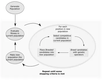
Figure 2.1: Example, high level description of a typical evolutionary algorithm.

by a chromosome’s representation of a city ordering. In this case, the smaller the distance travelled, thefitterthe chromosome. Calculating the fitness of the whole population is typically the bottleneck of the algorithm.

Selection is a method used to decide which chromosomes are to be propagated into the next

generation (next round of evaluations, selection, and genetic operators). There are multiple ways one could go about doing this, however the main objective is to select some relativelyfit

chromosomes. One should avoid simply selecting the most fit individuals as this typically sends the search into a local optimum and the algorithm will converge too quickly. To discourage the GA from converging too quickly, one wants to encourage a good level ofgenetic diversity— a population containing chromosomes somewhat distinct from one another.

Genetic operators are the methods applied to selected chromosomes when propagated into the next generation’s population. There are typically two genetic operators: crossover and

mutation. Crossover is designed to be somewhat analogous to processes which occur during sexual reproduction; two reasonably fit chromosomes will breed and produce two offspring which are somewhat similar to both parent chromosomes. Mutations, unlike crossover, occur on a single chromosome at a time and will alter the chromosome slightly in some way.

This process repeats many times until some termination criteria is met. This could be after some number of generations, after the algorithm has converged, or after some fitness value is obtained. Figure 2.1 depicts the execution flow of a typical GA/EA.

(22)

potentially stochastic in nature, and have no other reasonable means of computational based problem solving. GAs, and its variations, have been applied to many applications. Engineering and design has been accomplished with the design of buildings to minimize energy use [119], structural design of commercial buildings [90], synthesis of the antennas for NASA’s Space Technology 5 (ST5) mission [48, 86], NASA’s deep space communication networks [45], elec-trical circuit design [73], robot programming [75], and robot design/manufacturing or robotic lifeforms [83, 127].

2.1.1 Modular Enhancements

One of the major advantages of genetic algorithms is the modular nature of the methods. It is easy to alter and add operators to the algorithm to better fit the application. Alterations and additions are frequently created and some have since become standard in the literature. Below are a collection of typical enhancements incorporated in genetic algorithms.

Representation

Representations have become a widely studied area within the field as there are numerous ways to represent any given problem and some representations may have some inherit advantages over others.

Classically, a genetic algorithm’s representation of a candidate solution would be a string of 0s and 1s which would represent something meaningful with respect to the problem space. These 0s and 1s would be thegenotypeand would require some sort of translation into a phe-notype(something to be evaluated by thefitness function — the function which calculates the candidate solution’s fitness). With this binary representation John Holland introduced Hol-land’s schema theorem for exponential increases in fitness over successive generations [47]. This theorem essentially demonstrates the power and usefulness of GAs.

This indirect representationis by no means a requirement. Over time it became easier to implement other representations and more direct representations — where no translation is required — became feasible. For example, when studying the travelling salesman problem, instead of a binary string, one could implement an ordered list of cities directly representing the order to visit each city. Although these more complex representations do not strictly align to Holland’s schema theorem, they were shown early to be effective [42, 63].

Selection

Multiple selection algorithms for genetic algorithms exist and new ones are always being de-veloped.

One could always select the best chromosomes to breed and populate the next generation, however this approach tends to cause the GA to converge quickly into a local optimum. Alter-natively, one might implement a completely random selection, although this would eliminate the highselection pressureof the strong (relatively fitter) candidate solutions.

(23)

2.1. GeneticAlgorithms 11

Before Crossover

11111111111111

00000000000000

After Crossover

11111000000000

00000111111111

Figure 2.2: One point crossover example with a simple binary value representation. All values within the darker emphasised area are swapped between the two chromosomes. This figure also shows a simple binary representation.

Popular selection methods include proportional selection[47], tournament selection[43], andlinear ranking[7]. These, and more, have well studied effects on selection pressure [6].

Elitism

Despite the fact that selection algorithms make an effort to avoid always selecting the best chro-mosomes, it has become standard to propagate the most fit chromosome (sometimes more than one) into the next generation to preserve the best known solution. The best known chromosome will always be monotonically non-decreasing over time; it cannot be destroyed by stochastic changes [8].

Genetic Operators

The genetic operators are how the GA explores new areas of the search space and exploits already known highly fit chromosomes. These operators area easily changed and tuned to appropriately align to the specific problem the GA is being applied to. There are a number common techniques for both operators, however, new techniques are always being developed to exploit the intricacies of specific problem spaces.

Common crossover techniques includeOne-Point Crossover(depicted in Figure 2.2) (every element after an index is swapped between two parent chromosomes),Two-point crossover (ev-ery element between two indices are swapped between two parent chromosomes), andUniform Crossover(some number of indices are selected and all elements at these indices are swapped between the parent chromosomes). Some techniques are more destructive than others, and they all have their strengths and weaknesses.

Mutation only occurs on one chromosome at a time. Common mutation techniques include a single/multi-point mutation (select random indices and replace them with new values from the set of available values), exchange mutation (swap two or more elements), and updates (altering real value elements with an increment/decrement).

(24)

Migrations

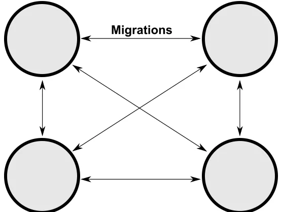
Figure 2.3: In this example, each circle represents a separate population (4 in this case) which evolve independently from one another. After some number of generations, chromosomes from each population have the opportunity to migrateto other populations. This particular figure shows allowable migrations between all populations, however this is not a requirement.

Distributed Populations

Distributing the search by dividing a population into multiple sub-populations has become pop-ular. This method attempts to simulatepunctuated equilibriaandallopatric speciation, or sim-ply, encouraging genetic diversity over thewholepopulation by allowing thesub-populations to traverse the search space along their own trajectories. This idea is sometimes called the

island model.

The general idea is to break the population down into sub-populations and execute a GA on each of the sub-populations with periodic information transfer between them. Multiple versions of these distributed systems exist. Figure 2.3 demonstrates a case with four sub-populations that is completely connected; information can be transferred, ormigrated, between any of these sub-populations.

The idea of distributing the search has existed for some time. Booker notes in his Doctoral Dissertation [14]:

Two separate populations are used rather than one large one so that the learning al-gorithms can benefit from having classifiers already separated into gross functional “niches.”

(25)

2.2. GeneticProgramming 13

*

-1.2

x

y

(a)Function. Represents a mathematical expression, namely, this represents (1.2+

v1)∗v2.

<

length 5.2 red

not or

(b) Binary classification Program. Rep-resents some binary classification, namely, (LENGTH<5.2)|notRED

if

and

open _closedright forward turn

right

(c) Represents a program, namely,

if(OPEN & RIGHT CLOSER)then FOR-WARDelseTURN RIGHT.

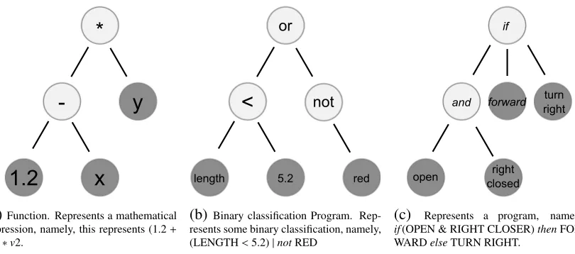
Figure 2.4: Three exampleprogramsrepresented in a tree-structure.

Fitness Approximation

The fitness evaluation of each chromosome is, in most cases, the most computationally expen-sive portion of the evolutionary search.

It can be advantageous to use a method which canquicklyapproximate the fitness of a chro-mosome or a collection of chrochro-mosomes. There are a number of approaches to this within the literature, and many are not restricted to just evolutionary searchers. Some popular approaches include sub-sampling the data, fitness inheritance (inherited fitness values from parent chro-mosomes) [107],fitness imitation(cluster chromosomes and evaluate only representative chro-mosomes) [68, 66], andpartial evaluation(a combination of fitness inheritance and imitation) [99]. These, and other techniques are reviewed in [66].

As stated in [105], these techniques are beneficial as they can reduce the complexity of the problem, eliminate the need for an explicit fitness function (some problems don’t have an explicit evaluation method), reduces the concerns of a noisy fitness function, smooths the fitness landscape (reduces the number of local optima), and promotes genetic diversity.

2.2 Genetic Programming

As interesting and creative representations for GAs became more popular, a tree structure rep-resenting computer programs was implemented [25]. John R. Koza expanded upon the idea of using a tree structure representation and ultimately developed the field ofGenetic Program-ming (GP); using evolutionary search to explore the space of functions/computer programs [69, 70, 71, 72, 75, 73, 74].

(26)

+

-1.2 x

2.0

*

-3.1

x

-2.2 x

+

-1.2 x

2.0

*

-3.1

x

-2.2

x

Before Crossover After Crossover

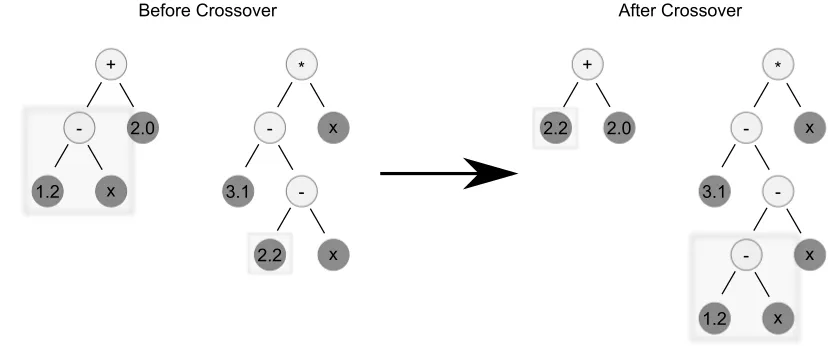
Figure 2.5: Example of a one point crossover operation between two tree-structure chromo-somes.

— symbolic regression2 — then the fitness may be the mean squared error calculated when applying the expression to data. If Figure 2.4b was some decision tree for binary classification, the fitness could be the percent accuracy. If the program in Figure 2.4c is describing how a robot should manoeuvre to solve a maze, then the fitness may how close the robot got to the exit3_.

Special genetic operators are also required for these tree structures. A common approach would be to select sub-trees from each chromosome and swap them. Figure 2.5 demonstrates this sub-tree exchange. This is a very similar technique to one-point crossover, a common crossover technique with basic GAs. Mutation could be a single point mutation (select a node and change it), or an exchange mutation (select two nodes and swap them within the same chromosome). Similar to GAs, new genetic operators are developed for GP constantly.

The operators and operands that are used in the representation are defined by a language

(basis functions). Languages are selected for the problem being solved. If one was performing symbolic regression then an appropriate language may be+, −, ∗, /, log, exp, variables, and

floating point number constants. If a decision tree was to be developed, a more appropriate language may be the logical operators, real numbers, and the variables. Note that in the latter example there are multiple types (Boolean and Numerals). A GP system with multiple types (typed GP) has additional requirements on the genetic operators as they need to preserve node return types.

GP is in no way limited to a tree structure. Linear Genetic Programmingis an alternative which treats the representation as a sequence of instructions from an imperative, or machine language. This differs from the more functional implementation of the tree structure. Other noteworthy representations exist, including graph based representations (more on this in Sec-tion 2.2.1).

Notable early applications of GP are reviewed in [71, 72, 74], and include quantum

com-2_{A type of regression analysis often performed with GP that searches for the whole model (operators,}

coeffi-cients, structure, feature selection) as opposed to just coefficients.

(27)

2.2. GeneticProgramming 15

puting [9, 112, 109, 110, 111], robot programming [3, 87], bioinformatics [71], engineering, and circuit design [71].

2.2.1 Acyclic Graph Representation

An acyclic graph representation for symbolic regression was studied and compared to the traditional tree structure by Schmidt et al. in [102]. Other graph encodings (either explicit or implicit) for GP have existed for some time [98]. One of the most popular isCartesian GP [93, 91, 92], however, Schmidt et al.’s gives some unique advantages (although this is entirely implementation dependent).

Figure 2.6 presents a comparison of a tree representation and an acyclic graph representa-tion. These structures represents the following equation: (1.23− x)+sin((1.23− x)·y·ex), wherexandyare variables.

This representation, when compared to the tree representation, scales better, has a lightweight array encoding, and avoids bloat — the tendency of evolved programs to grow arbitrarily large without significant improvement in fitness [98]. Additionally, it can easily reuse possibly im-portant sub-expressions and can maintain vestigial information within the encoding which may resurface effectively in future generations.

It was also noticed that this acyclic graph representation converges slower (although this may be considered an advantage) and is susceptible to deleterious crossovers [102]. However, their results strongly demonstrate the benefits of this representation.

2.2.2 Fitness Predictors

Fitness Predictors, a fitness approximation approach, were studied by Schmidt el al. in [104, 105] and it was demonstrated that they can reduce computational cost by approximating the local search gradient.

The candidate solutions are evaluated with an adaptive subset of the data as opposed to all data. If the subset of data can sufficiently describe the whole, then it can be used as an effective approximation of fitness. Using a subset in the realm of 10% the size of the whole data set can greatly reduce the number of evaluations required to determine fitness values. This value is parameterized and os typically determined empirically with preliminary testing.

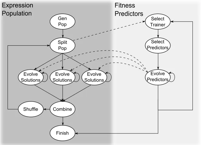
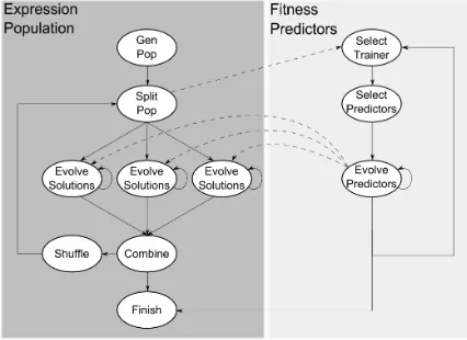
The fitness predictors are adapted by evolving alongside the candidate solutions, and the fitness predictors’ fitness value is determined by a measure of how well it can approximate the whole data set. Additionally, this method also attempts to select the data points in a way which creates a large variance in the fitness of candidate solutions on fitness predictors through the use offitness trainers. In other words, the subset of data points are selected in a way to focus the search on areas of the search space where the candidate solutions are less effective. Figure 2.7 presents an overview of how these fitness predictors would evolve alongside the evolutionary search.

(28)

1.2

+

*

-sin

e^

x 1.2 x

y

x

(a)A mathematical expression using a tree representa-tion. 13 are used to represent this expression. Every part of this expression must be explicitly represented with a node.

+

*

-sin

e^

1.2

y

x

(b) A mathematical expression using an acyclic graph representation. 9 nodes were used to represent this ex-pression. Notice how the sub-expression (1.23−x) is easily reused.

1.2 x

? ?

e -y

?

*

? ?

*

? ?

sin

? ?

+

(c)Example encoding of the acyclic graph representa-tion. Root is at the bottom, and all children must exist above the parent. ’?’ represent currently unused infor-mation within the structure.

Figure 2.6: Figures 2.6a and 2.6b both represent the same expression: (1.23−x)+sin((1.23−

(29)

2.3. GeneticProgrammingImplementation 17

Gen Pop

Expression Population

Fitness Predictors

Select Trainer

Evolve Solutions

Combine

Select Predictors

Evolve Solutions

Evolve Solutions Split

Pop

Shuffle

Evolve Predictors

Finish

Figure 2.7: High level overview of a GP system implementation with fitness predictors evolv-ing in parallel. This particular example contains multiple sub-populations.

In addition to the performance enhancement of a reduction in computation cost through using a small subset of data points for evaluation, fitness predictors have been shown to produce better quality results by reducing overfitting. Overfitting is curbed since evolution is always based on the fitness of an ever evolving subset of data points; overfitting becomes difficult when the target points are always changing.

It has also been shown that symbolic regression performs better when allowed to focus on key features (subsets of data) as opposed to the whole data set [104, 105].

2.3 Genetic Programming Implementation

The papers in Chapters 4, 5, and 6 contain brief descriptions of the GP implementation and parameter settings used. In summary, the GP system built for this work incorporates multiple enhancements to improve the search capability of the evolutionary algorithm and were ulti-mately required in order to effectively traverse the large space in a reasonable amount of time. These enhancements include: elitism, an acyclic graph representation [102], fitness predictors [104, 105], and parallel evolution of subpopulations. Figure 2.7 provides a high level overview of the algorithmic flow of the implemented GP system. A GitHub repository of the GP system

(30)

Functional Magnetic Resonance Imaging

Data and Literature Review

MRI is a technology which harnesses magnetic fields to create images of anatomy and physio-logical processes within a body. MRI uses nuclear magnetic resonance in a controlled way

to generate 1 – 5mm3 voxels — three-dimensional volume elements analogous to a

two-dimensional pixel — containing information about the spin-relaxation properties of atomic particles within the voxels. This information can be used to distinguish tissue types and prop-erties [16, 26].

MRI works by aligning protons within a body with a very strong magnetic field, applying electromagnetic (EM) energy at a resonance frequency such that specific atomic particles ab-sorb it, and then recording the resulting particle activity [50]. Whether the MRI technology is being used to generate structural images of the brain or the functional moment-to-moment changes within the brain, the high level idea is the same. For the interested reader, a thorough discussion of the underlying technology and phenomenon can be found in [16].

A large static magnetic field is used to align a small, but not insignificant number of protons (the atomic nuclei within the hydrogen atoms in water). Typically, the magnetic field used for MRI is created by passing a current through a coil of superconducting wire. Modern scanners can generate and maintain static magnetic fields between 1.5 – 11T for humans (realistically, it is common to see 1.5T and 3T scanners), and up to 24T for animals. The earth’s magnetic field is on the order of 0.0001T (between 25 – 65µT).

The static magnetic field does not create any magnetic resonance signal, but the application of resonant EM radiation to the aligned protons and resulting reaction does. EM radiation (photons) tuned to a specific frequency is applied to the body within the scanner such that some protons absorb the energy and enter an excited state. The specific frequency is selected to be the resonant frequency for the target particle, typically hydrogen nuclei. When the application of the EM radiation is stopped, the excited protons will eventually return to align with the magnetic field, and in doing so, will releaseenergy over timethat can be recorded.

The way this is measured will record different signals that may be suited for structural or functional imaging. The important part is that with the application of EM radiation, a collection of particles will react a predictable way, and the results can be measured to indicate blood oxygen levels. With the clever use of controlled spatial variations in the magnetic field strength, the recorded signal can be spatially localized. Localized variations in the blood oxygen levels

(31)

19

are of interest as they can be used as a proxy for brain activation.

Functional magnetic resonance imaging(fMRI) is a neuroimaging modality used to mea-sure functional brain activity with the BOLD signal. The BOLD signal is a meamea-sure of the relative(de)oxygenation level of blood within tissue resulting from an increase in blood flow to cerebral tissue which correlates with neural activation (a result of the HDR) [79, 95, 50]. This is believed to happen because neurons do not store their own energy and oxygen and must depend on the vascular system to replenish resources.

The actual nature of the BOLD signal is not entirely understood, and it should be noted that fMRI is in reality measuring a phenomenon that lags behind electrical recordings of neural actively by a few seconds and is spatially diffused; the surrogate signal is based on to the blood flow of surrounding tissue of recent activity. However, it has been firmly demonstrated that this signal is strongly linked with the underlying neural activity [85], but ultimately there are physical and biological limitations to the signal which are consistently under-represented, many of which are reviewed in [5, 46, 84].

fMRI data is four-dimensional; it contains the three-dimensionalanatomical space along with the changes in activation overtime. Depending on the technology, the anatomical space is measured from 1 – 5mm3and changes in time are sampled every 0.5 – 3s; modern scanners are capable of capturing at a frequency of 0.75 – 2Hz. Although the resolution each voxel is on the order of millimetres, each voxel contains tens of thousands of neurons. For this reason they can be thought of as a “mesoscale” representation; it lies between the microscale of neurons and the macroscale of brain lobes.

fMRI is particularly popular as it is non-invasive and has relatively high spatial resolution when compared to other imagining technologies. fMRI allows researchers to ask which brain regions are involved in tasks/stimulus, how they relate to one another, and how they com-municate. This technique has been used to ask many interesting behavioural, physiological (functional and structural), clinical questions.

In task-based fMRI, tasks or stimulus are presented to a subject and the corresponding measured signal (BOLD) is compared to the expected HDR [1, 30]; what we expect a measured signal to look like if it were responding to some presented stimulus. Areas of the brain (voxels or other ROI) whose signal corresponds to the expected HDR is said to have been activated by the task/stimulus [18, 96, 101, 49]. Any timeseries metric could be used for comparing the BOLD signal to the expected HDR, however the GLM (general linear model) is very common. The general linear model is a linear model of the form Y = BX +U, where Y is a matrixof dependent variables, X is a matrix of independent variables, B is a matrix of parameters (to be found), andU is a matrix of errors/residuals. Effectively, it is a generalization of multiple linear regressions for many dependent variables.

Figure 3.1 depicts an HDR function; if a voxel/ROI’s measured BOLD signal were to lin-early correlate with this spiking event then it is said to be activated by the stimulus.

(32)

Timeu~25-39s

Intensity

Sometimesuthere isuanuinitialudipuhere

Signalupeaku betweenu~4-8s

Returnsutoubaselineu atuaroundu10s

Undershootumay appearuforusome time

Event

Figure 3.1: Hemodynamic Response Function [15]. After an event/neural spike, the relative deoxygenated blood levels increases (sometimes with an initial dip before the increase) and after roughly 10 seconds, levels returns to close to baseline.

limited to, self-referencing, self-memory, thinking of others, moral reasoning, social and moral reasoning, remembering the past, and planning the future [4]. Additionally, these resting-state networks also have significant clinical implications with respect to better understanding of mental illnesses such as Alzheimer’s, and schizophrenia [17, 88, 100, 113].

3.1 Graph Theory

When studying these brain relationships, neuroscientists began simplifying their data and anal-ysis by reducing the four-dimensional fMRI data into a static graph — a set of vertices and edges — representing functional or structural connectivities. With this, graph properties, such as vertex degree or distance, become easy to study.

Interesting early discoveries with this graph approach include network motifs [115], and the prevalence ofsmall world propertieswithin these connectivities [11]; graphs with densely connected clusters and a small number of connections between clusters [124].

This approach has become increasingly popular and many of the methods can be viewed in these review papers [19, 28, 114].

3.1.1 Discovering Relationships

(33)

3.2. PreviousWork onNonlinearRelationships 21

random matrix theory [26].

It is interesting how well linear models can describe the relationships within the system, given that the brain is a nonlinear computing system as it is Turing-complete. Perhaps a sig-nificant portion of the relationships are linear; there has been work done with these linear tools and the majority of the meaningful relationships appear to be linear [108]. Noise has also been demonstrated to obscure potentially important nonlinearities [29]. Additionally, it has been noted that the BOLD response is a nonlinear integrator [121, 123, 82].

3.2 Previous Work on Nonlinear Relationships

Below is a collection of works by various authors exploring nonlinearities within fMRI data. This collection is by no means exhaustive and each individual work includes a literature review of similar research. The last work in this section is the most relevant to this thesis as it is the most similar; it studies the brain from a network/graph perspective and attempts to describe the network relationships using symbolic regression (see Section 2.2).

Buxton et al. describe theBalloon model, a nonlinear input-output model of blood flow and oxygenation changes where input is blood flow and output is the BOLD signal [20, 22]. The simplistic biophysical model of the HDR was used in a finger tapping task-based fMRI study to capture essential features of the BOLD signal.

Nonlinear models for the BOLD signal were studied with Volterra series expansion by Friston et al. [36, 37]. They develop a nonlinear model of the BOLD signal using Volterra series expansion, a model-independent method capable of modelling the behaviours or any nonlinear time invariant dynamic system [36]. They show that the Balloon model can account for nonlinearities in event-related responses. They also describe a nonlinear dynamic model of the relationship between synaptic activity and fMRI signals. This model incorporates the Balloon model and is characterized in terms of it’s Volterra kernels. They argue that the kernel parameters are biologically plausible and are sufficient to account for a number of nonlinearities in the data.

Deneux and Faugeras studied variations of the balloon models (such as those discussed in [22, 21, 37]) and physiological plausible models and their use in fMRI data analysis. They suggest that their models better describe the BOLD response when compared to linear tools, but are comparable when being applied to noisy data [29].

Kruggel et al. used fMRI data recorded from an event related item recognition experimental design [77]. After preprocessing, the authors used linear regression to find areas of functional activation within the data to select ROIs. Once the areas of interest were selected, they used nonlinear regression to quantify the relationships between the stimulus and the BOLD signal’s shape. The nonlinear regression used in the work was developed by Kruggel and von Cramon for modelling nonlinearities within fMRI data (described in [78]). They note that the success of a nonlinear analysis of the data is dependent on a well thought out collection of model equations and conclude that their presented approach achieves afinerdescription of the fMRI experiments and hope that it will lead to new insight into cognitive neuroscience.

(34)

The work was extended by Stephan et al. to perform a more general nonlinear dynamic causal model [117]. More up-to-date information regarding the project can be found at:http://www. scholarpedia.org/article/Dynamic_causal_modelling[89]. The extended nonlinear dynamic causal model was capable of distinguishing nonlinear and bilinear processes when applied to synthetic fMRI data. The models were also applied to real fMRI data gathered from a motion task to analyze nonlinearities, namely,gating— the response of a neuron to activity is dependent on the history of inputs from other neurons.

Wager et al. show nonlinear effects in fMRI BOLD signal when a rapid event-related ex-perimental design is used (1s apart) [123]. Their interest was in nonlinearities introduced by stimulus history and they developed a low-dimensional parametrization of nonlinearities in re-sponse magnitude, time to peek, and rere-sponse onset time. The authors demonstrate that their model is more accurate and reasonably consistent across the brain. They argue the importance of accounting for nonlinearities when focused on subject specific analysis relative to a group analysis since inaccurate linear models of the nonlinear phenomenon for the group could create biases when applied across participants.

Zhang et al. used a nonlinear semi-parametric model built around Volterra series to char-acterize measured BOLD signal and found deviations from the linear models [126]. They applied the method to real fMRI data from a monetary incentive delay experiment [67] and showed that their approach outperformed many existing methods. They acknowledge the dif-ficulty in selecting the number of parameters for describing nonlinearities with their approach, and therefore they limit the number of functional bases (free parameters).

In 2015 Nicholas Allgaier used symbolic regression as a means to discover nonlinear rela-tionships within resting-state fMRI data [2]. This particular work is the most relevant to this thesis as it is using the same underlying technique to discover nonlinearities and studies them as a network; however, there are important distinctions1_{. The authors studied known networks}

within resting-state data to develop nonlinear models. 52, 9mm3 ROIs were selected based on the DMN. It was found that their nonlinear terms generated in the models better account for variance when compared to traditional linear tools. It was also found that the most com-mon relations modelled corresponded to knownintrinsic connectivity networks. Similar work was also done by Icke et al. in [61] which hybridized GP with deterministic techniques with success. They also suggest that symbolic regression alone has too many shortcomings to be effective for modelling nonlinearities in fMRI data. Other unpublished works from the same lab also analyze some small sample task-based studies.

3.3 Details on Data Used

As discussed in Chapter 1, task-based fMRI timeseries data was obtained from the Human Connectome Project and segmented into 30 ROIs. Figure 1.1 provides a view of the ROIs and Table 3.2 names the neuroanatomical regions of the 30 ROIs.

Tasks performed for the Human Connectome Project’s task-based fMRI data include: Emo-tion, Gambling, Language, Motor, Relational, Social, and Working Memory.

Table 3.1 provides an example of how the data can be represented simply in tabular format.

Finding Nonlinear Relationships in Functional Magnetic Resonance Imaging Data with Genetic Programming

Scholarship@Western

Scholarship@Western

Finding Nonlinear Relationships in Functional Magnetic

Finding Nonlinear Relationships in Functional Magnetic

Resonance Imaging Data with Genetic Programming

Resonance Imaging Data with Genetic Programming

Co-Authorship Statement

Contents

List of Figures

List of Tables

Chapter 1

Introduction

1.1

fMRI Data

1.1.1

Graph Interpretation

1.1.2

Human Connectome Project Data

1.2

Neuroscientific Motivation

1.3

Methods

1.4

Nonlinear Analysis of fMRI data

1.5

Contribution

1.6

Thesis Format

Evolutionary Computation and Literature

Review

2.1

Genetic Algorithms

2.1.1

Modular Enhancements

Before Crossover

11111111111111

00000000000000

After Crossover

11111000000000

00000111111111

*

-1.2

x

y

<

2.2

Genetic Programming

2.2.1

Acyclic Graph Representation

2.2.2

Fitness Predictors

2.3

Genetic Programming Implementation

Functional Magnetic Resonance Imaging

Data and Literature Review

3.1

Graph Theory

3.1.1

Discovering Relationships

3.2

Previous Work on Nonlinear Relationships

3.3

Details on Data Used