Title: Detection and Recovery of Faulty Nodes Using Clustering Optimization and Bayesian Analysis in Wireless Sensor Networks

(1)

227

Available Online atwww.ijcsmc.com

International Journal of Computer Science and Mobile Computing

A Monthly Journal of Computer Science and Information Technology

ISSN 2320–088X

IMPACT FACTOR: 6.017

IJCSMC, Vol. 6, Issue. 5, May 2017, pg.227 – 234

Detection and Recovery of Faulty Nodes

Using Clustering Optimization and Bayesian

Analysis in Wireless Sensor Networks

Beena.T

1

, Biju Balakrishnan

2

¹PG student, Computer Science and Engineering, Nehru Institute of Technology, Coimbatore, India ²Assistant Professor, Computer Science and Engineering, Nehru Institute of Technology, Coimbatore, India

1

[email protected]; 2 [email protected]

Abstract: An WSN may often consist of hundreds of distributed sensors to monitor, collect and transmit information from various environments. Signals are relayed from one sensor to another sensor until it reaches the sink node which could

either be mobile or a central controlunit. The breaking down of sensors would inevitably affect the transmission of signals

or even cause signal lost. Hence it is normal that inactive nodes miss their communication in network hence split the network. The clustering optimization technique efficiently groups the nodes into clusters and selects a cluster head based on the maximum energy. The number of members is limited based on the communication distance and the number of cluster per network is also constrained to number of nodes in the network. The fault nodes are detected based on the signals collected from them and classified into scene fault and node fault. The data from the fault nodes are recovered by using Bayesian analysis of compressive sensing to the cluster head. The secondary cluster head is chosen based on energy level and it takes the position of cluster head in the case of failure of the head. This approach allows faulty nodes recover their data by selecting neighbourhood cluster properly and increases detection accuracy of fault diagnosis and reduces time complexity.

Keywords: Clustering, Cluster head, Fault diagnosis, Secondary cluster head

I.INTRODUCTION

(2)

228

connectivity changes over time, to forward a packet reliably at each hop, it may need multiple retransmissions. This results in undesirable delay as well as additional energy consumption.

A sensor node in wireless sensor network that is capable of performing some processing, gathering sensory information and communicating with other connected nodes in network. The main components of a sensor node are a microcontroller, transceiver, external memory, power source and one or more sensors. A sensor node in wireless sensor network that is capable of performing some processing, gathering sensory information and communicating with other connected nodes in network. The main components of a sensor node are a microcontroller, transceiver, external memory, power source and one or more sensors.

Most transceivers operating in ideal mode have a power consumption almost equal to the power consumed in receive mode. External memory used for storing application related or personal data and program memory used fpr programming the device.

An important aspect in the development of a wireless sensor node is ensuring that there is always adequate energy available to power the system. The sensor node consumes power for sensing, communicating and data processing. More energy is required for data communication than any other process. Sensors are hardware devices that produce a measurable response to a change in a physical condition like temperature or pressure. Sensors measure physical data of the parameter to be monitored. The continual analog signal produced by the sensors is digitized by an analog-to-digital converter and sent to controllers for further processing.

II. RELATED WORKS

The sensor nodes in wireless sensor networks may be deployed in unattended and possibly hostile environments. The ill-disposed environment affects the monitoring infrastructure that includes the sensor nodes and the network in addition to node failures and network partitioning. This in turn adds a new dimension to the fragility of the network topology. Such perturbations are far more common than those found in conventional wireless networks thus, demand efficient techniques for discovering disruptive behavior in such networks.[1]Traditional fault diagnosis techniques devised for multiprocessor system are not directly applicable for WSN due to their specific requirements and limitations. The fault diagnosis techniques are classified based the nature of the tests, correlation between sensor readings and characteristics of sensor nodes and the network.Distributed self diagnosis is an important problem in wireless sensor networks (WSNs) where each sensor node needs to learn its own fault status. The classical methods for fault finding using mean, median, majority voting and hypothetical test based approaches are not suitable for large scale WSNs due to large deviation in inaccurate data transmission by different faulty

sensor nodes. [11]One of the most critical issues is the detection of corrupted readings amidst the huge amount of gathered sensory data. Indeed, such readings could significantly affect the quality of service (QoS) of the WSN, and thus it is highly desirable to automatically discard them. This issue is usually addressed through “fault detection” algorithms that classify readings by exploiting temporal and spatial correlations[3]Fault detection, isolation, and estimation are considered for a class of discrete time- varying networked edge sensing system with incomplete measurements.

III. EXISTING SYSTEM

Wireless Sensors Networks (WSN) fault diagnosis problem is formulated as a pattern classification problem and introduces a newly developed algorithm, Neighborhood Hidden Conditional Random Field (NHCRF), for determining hidden states between sensors. The health conditions of WSN are determined by using the NHCRF model to estimate the posterior probability of different faulty scenarios. The NHCRF model can improve the WSN fault diagnosis because it has relaxed the

Transceiver

Micro-controller

External memory Power

source

Sensor 1

ADC

(3)

229

independence assumption of the Hidden-Markov model. To enhance the robustness and anti-noise ability of the NHCRF, the concept of nearest neighbors is used when estimating dependencies. In this paper, a 200-sensor-node WSN is used to show that the proposed NHCRF method can deliver excellent and effective results for WSN-health diagnosis.[1] The contributions of this paper are three-fold. First, a new algorithm called Neighborhood Hidden Conditional Random Field which is derived for handling fault diagnosis such as locating faulty nodes in an WSN. Second, in contrast to other conventional methods that mainly detect faulty sensor nodes, our proposed NHCRF algorithm and its relaxed characteristic enables hidden states of an WSN be determined. Thus, the dependencies among sensors and transmission paths are found. And as a result, faulty scenes caused by faulty transmission path but not sensor nodes can also be detected. Third, only neighborhood dependencies rather than global dependencies are used for detecting states of hidden variables. This eliminates the effect caused by distant neighbors, and thus enhances the robustness of diagnosis significantly. Different from the previous fault diagnosis methods employing many metrics collected by extra devices monitoring the sensors in an WSN, the proposed diagnosis approach relies only on the collected signal delay data.

IV. PROPOSED SYSTEM

Some WSN with a lot of immobile node and with the limited energy and extension of many sensor nodes and their operation. Hence it is normal unactive nodes miss their communication in network, hence split the network. For avoidance split of network, we proposed a fault recovery corrupted node and Self Healing is necessary. In this Thesis, a design techniques to maintain the cluster structure in the event of failures caused by energy - drained nodes. Initially, node with the maximum residual energy in a cluster becomes cluster head and node with the second maximum residual energy becomes secondary cluster head. Later on, selection of cluster head and secondary cluster head will be based on available residual energy. Sensors provide an easy solution to those applications that are based in the inhospitable and low maintenance areas where conventional approaches prove to be impossible and very costly. Sensors are generally equipped with limited data processing and communication capabilities and are usually deployed in an ad-hoc manner to in an area of interest to monitor events and gather data about the environment. Sensor nodes are typically disposable and expected to last until their energy drains. Therefore, it is vital to manage energy wisely in order to extend the life of the sensors for the duration of a particular task. Failures in sensor networks due to energy depletion are continuous and may increase. This often results in scenarios where a certain part of the network become energy constrained and stop operating after sometime. Sensor nodes failure may cause connectivity loss and in some cases network partitioning in clustered networks, it creates holes in the network topology and disconnects the clusters, thereby causing data loss and connectivity loss. Good numbers of fault tolerance solutions are available but they are limited at different levels.

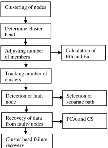
Fig 2:Architecture of clustering and detection of fault nodes

Clustering of nodes

Adjusting number of members

Calculation of Eth and Eic

Recovery of data from faulty nodes Determine cluster head

Tracking number of clusters

Selection of separate path Detection of fault

node

Cluster head failure recovery

(4)

230

The clustering of nodes in a network is done based on energy levels and the neighboring information. Then the cluster head is determined based on the higher level of nodes and a secondary head is selected based on the secondary energy level. Data from the fault nodes can be recovered using Bayesian analysis of compressive sensing to the cluster head. The number of members in a cluster is limited to a constraint and the number of clusters in a network is limited according to the network size. The detection of fault node is done based on the energy level and if fault node is found in the path then a separate path is found.

Algorithm ComputeNI (graph G(N,L))

// N: set of graph nodes, L: set of links between these nodes // Output: Array NI[·]: NI index value for each node of N begin

NI[t] = 0, ∀t ∈ N;

foreach( n ∈ N ) do { S: an empty stack;

P[·]: array of empty lists (one list ∀ node w ∈ N); σ[·]: an array, where σ[t] = 0, ∀t ∈ N; σ[n]=1; d[·]: an array, where d[t] = −1, ∀t ∈ N; d[n]=0; Q: an empty queue;

Q.enqueue(n);

while( Q.isNotEmpty() ){ v = Q.dequeue(); S.push(v);

foreach 1-hop neighbor w of v do //w found for the first time? if( d[w] < 0 ) then

Q.enqueue(w); d[w] = d[v] + 1;

// shortest path to w via v? if( d[w] == (d[v] + 1) ) then σ[w] = σ[w] + σ[v]; P[w].append(v); }δ

[·]: an array, where δ[t] = 0, ∀t ∈ N;

// S returns nodes in order of non-increasing hop distance from n while( S.isNotEmpty() ) do

w = S.pop();

foreach( v ∈ P[w] ) do δ[v] = δ[v] + σ[v] σ[w] ∗ (1 + δ[w]); if( w _= s )

NI[w] = NI[w] + δ[w]; }

return NI; end

The clustering optimization is done by clustering the nodes in the network based on some constraints such as sensing range, transmission range, network size and number of nodes. The clustering information is stored in the queue and stacks in the program. The nodes are ordered based on the neighboring node distance with each node containing next hop information.

A. Cluster formation

(5)

231

B. Determining cluster head

The node with highest energy level is choosen as a cluster head. Every cluster head sends a message cluster_head_status msg and Eic to its neighbours (within sensing range) and every cluster head keeps a list of its neighbor cluster heads along with its Eic. The nodes which receive Eic lesser than itself relinquishes its position as a cluster head. The cluster heads which are active send their messages to the cluster head manager outside the network. The cluster_head_manager has the information of the desired cluster head count. If the number of cluster heads are still much more than expected, then another round of cluster head relinquishing starts. This time the area covered would be greater than sensing range. The area covered for cluster head relinquishing keeps increasing till the desired count is reached.

C. Adjusting number of members

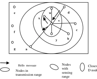
Nodes send a message hello_msg along with their coordinates which are received by nodes within the transmission range. For example in figure (1) nodes a,b,c,d,w,x,y are within transmission range of v.After receiving the hello_msg, the node v calculates the distance between itself and nodes a,b,c,d,w,x,y using the coordinates from hello_msg. It stores the distance di and the locations in the dist_table.. Nodes within the sensing range are the neighbours of a node. In figure (1) nodes w,x,y,b are neighbours of v. Among the nodes within the sensing range, it chooses the first D closest neighbours as its potential candidates for next hop. Assuming D=3, in figure (1), the closest neighbours of v are w,x,y.

Fig 3: Clustering of nodes

Among the potential candidates, the farthest node‟s distance, dmax is taken for the calculation of E th .Suppose a node needs power E to transmit a message to another node who is at a distance „d‟ away, we use the formula E = E = kd c where k and c are constants for a specific wireless system. Usually 2 < c <4. In our algorithm we assume k = 1, c = 2. For a node v, d *1*d2max = Ethv, since there are D members to which a node sends message. Eic is the total energy spent on each of link of the D closest neighbours. For a node v, where k= 1. div is the distance between node i and node v. After the calculation of threshold energy Eth, nodes become eligible for cluster head position based on their energies. A node v becomes eligible for the cluster head position if its Einit > Ethv. and. node with the second Einit > Ethv becomes secondary Cluster head.. When no nodes satisfy this condition or when there is insufficient number of cluster heads, the admissible degree D is reduced by one and then Eth is recalculated. The lowest value that D can reach is one. In a case where the condition Einit > thv is never satisfied at all, clustering is not possible because no node can support nodes other than itself. There may also be situations where all the nodes or more number of nodes are eligible for being cluster heads. A method has been devised by which the excess cluster heads are made to relinquish their position.

D. Tracking number of clusters in a network

The size S of the cluster is tracked by each and every node. The cluster head accounts for itself and equally distributes

S-1 among its next hop neighbors by sending a message to each one of them. The neighbours that receive the message account for themselves and distribute the remaining among all their neighbours except the parent. The messages propagate until they reach a stage where the size is exhausted. If the size is not satisfied, then the algorithms terminates if all the nodes have been covered. After the cluster formation, the cluster is ready for operation. The nodes communicate with each other for the period of network operation time.

Hello message

Nodes in transmission range

Nodes with sensing range

Closest D nodes

g f e

x

b y

a

v

c

(6)

232

E. Detection of fault nodes

Signals are relayed from one senor to another sensor until it reaches the sink node which could either be mobile or a central control unit. Due to the low cost and the deployment of sensor nodes often in a harsh and uncontrolled environment, it is not uncommon that sensors would easily become faulty sensor nodes. The breaking down of sensors would inevitably affect the transmission of signals or even cause signal lost. Therefore, a lot of research has been done to improve the robustness of WSN fault diagnosis issue as a pattern classification problem.

Fig 4: Detection time decreases when clustering is used

The detection time used for finding faulty nodes get reduced as the entire network is divided into clusters. It uses signals collected from sensors, such as signal strength and frequency, and signal delay as features for classifying whether or not an WSN suffers from faulty sensors. The health conditions of WSNs can be determined by many attributes, e.g., package lost, radio interferences, package size, data collision on physical layer, etc. All of these measurements, however, cannot be easily obtained in real-world applications, especially for those sensors working in severe environmental conditions. The diagnosed result are classified into either node fault or scene fault.

F. Recovery of data from fault nodes

The task of accurately reconstructing a distributed signal through the collection of a small number of samples at a data gathering point using Compressive Sensing (CS) in conjunction with Principal Component Analysis (PCA). Our scheme compresses in a distributed way real world non-stationary signals, recovering them at the data collection point through the online estimation of their spatial or temporal correlation structures. The recovery of data is characterized under the framework of Bayesian estimation and it shows under the assumptions which is equivalent to optimal maximum a posteriori (MAP) recovery. The delay time get reduced as the data from fault nodes are recovered rather than finding and resending the packets again.

Fig 4: Delay time decreases when data is recovered so that packets are delivered successfully

G. Principal component analysis

(7)

233

method to represent through the best M-terms approximation a generic N-dimensional signal, where N > M, given that we have full knowledge of its correlation structure. In practical cases, i.e., when the correlation structure of the signals is not known apriori, the Karhunen-Lo`eve expansion can be achieved thanks to PCA [6], which relies on the online estimation of the signal correlation matrix. We assume to collect measurements according to a fixed sampling rate at discrete times k = 1, 2, ,K.

H. Compressive sensing

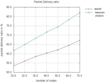
It is a technique that exploit to recover a given N- dimensional signal through the reception of small number of samples L smaller than N Invertable transformation matrix of size NXN such that N dimensional vector S(k) is sparse. Routing matrix is determined to find the way in which sensor data is gathered and transmitted by sink. CS is the technique that we exploit to recover a given N-dimensional signal through the reception of a small number of samples L, which should be ideally much smaller than N. The signals representable through one dimensional vectors x(k) ∈ RN, containing the sensor readings of a WSN with N nodes. The packet delivery ratio increases when the data is successfully recovered from fault nodes using compressive sensing.

Fig 6: Packet Delivery Ratio increases when data is recovered and transmitted

V.CONCLUSION

The clustering optimization technique efficiently groups the nodes into clusters and selects a cluster head based on the maximum energy. The number of members is limited based on the communication distance and the number of cluster per network is also constrained to number of nodes in the network. This project is carried out with two phases. In the first phase,the clustering is done and the fault nodes are detected based on the signals collected and classified into scene fault and node fault..This approach allows faulty nodes detection by the cluster properly and increases detection accuracy of fault diagnosis and reduces time complexity. In second phase, it recovers the data from fault nodes using Bayesian analysis of compressive sensing by the cluster head. The secondary cluster head is chosen based on energy level and it takes the position of cluster head in the case of failure of the head.

VI. FUTURE WORK

In future direction of research, various optimization approach for recovery of data can be implemented in order to improve the accuracy of the results. The energy efficiency can be enhanced by utilizing some improved mechanism.

REFERENCES

[1] Peng Tang, Tommy W. S. Chow,” Wireless Sensor Networks Conditions Monitoring and Fault Diagnosis Using Neighborhood Hidden Conditional Random Field‟‟, IEEE Transactions On Industrial Informatics, Vol. 11, No. 5,June 2016.

[2] Riccardo Masiero, Giorgio Quer, Michele Rossi and Michele Zorzi, “A Bayesian Analysis Of Compressive Sensing Data Recovery in Wireless Sensor Networks” on IEEE Transsaction on Industial Informatics, Vol.09, No. 5, May2016.

[3] Bill C.P. Lau, Eden W.M. Ma, Tommy W.S. Chow,” Probabilistic fault detector for Wireless Sensor Network,” Elsevier transactions on Expert Systems with Applications, 41(8), 3703-3711, June 2015

(8)

234

[5] Xiao He, Zidong Wang, Yang Liu, and D. H. Zhou,” Least-Squares Fault Detection and Diagnosis for Networked Sensing Systems Using A DirectS tate Estimation Approach ,” IEEE Transactions On Industrial Informatics, Vol. 9, No. 3, August 2013

[6] Safdar AbbasKhan , BoubakerDaachi, KarimDjouani,” Application of fuzzy inference systems to detection of faults in wireless sensor networks ,” Elsevier transactions onNeurocomputing 94 (2012) 111–120, February 2012.

[7] Jung Min Pak, Choon Ki Ahn, Yuriy S. Shmaliy, Myo Taeg Lim,” Improving Reliability of Particle Filter-Based Localization in Wireless Sensor Networks via Hybrid Particle/FIR Filtering ,” IEEE Transactions On Industrial Informatics, Vol. 11, No. 5, October 2015

[8] Kavita Tandon, Neelima Mallela, Nishi Yadav,” Novel Approach for Fault Detection in Wireless Sensor Network ,” International Journal of Computer Science and Information Technologies, Vol. 5 (2) , 2014, 2191-2194

[9] Abdulkadir Celik, Ahmed E. Kamal,” Multi-Objective Clustering Optimization for Multi-Channel Cooperative Spectrum Sensing in Heterogeneous Green CRNs,” IEEE Transactions on cognitive communications and networking DOI 10.1109/TCCN.2016.2585130, June 2016

[10] Abolfazl Akbar, Arash Dana, Ahmad Khademzadeh, Neda Beikmahdavi,” Fault Detection and Recovery in Wireless Sensor Network Using Clustering,” International Journal of Wireless & Mobile Networks (IJWMN) Vol. 3, No. 1, February 2011

[11] Mahapatro, A., & Khilar, P. M. (2013). Fault diagnosis in wireless sensor networks: A survey. IEEE Communications Surveys & Tutorials, 15(4), 2000-2026.

[12] Banerjee, I., Chanak, P., Rahaman, H., & Samanta, T. (2014). Effective fault detection and routing scheme for wirelesssensor networks. Computers & Electrical Engineering, 40(2), 291-306.

[13] Hodge, V. J., O'Keefe, S., Weeks, M., & Moulds, A. (2015). Wireless sensor networks for condition monitoring in the railway industry: A survey. IEEE Transactions on Intelligent Transportation Systems, 16(3), 1088-1106.

[14] Sahoo, M. N., & Khilar, P. M. (2014). Diagnosis of wireless sensor networks in presence of permanent and intermittent faults. Wireless Personal Communications, 78(2), 1571-1591.

Title: Detection and Recovery of Faulty Nodes Using Clustering Optimization and Bayesian Analysis in Wireless Sensor Networks﻿

227