FDTD Analysis of Rectangular Waveguide in Receiving Mode as EMI Sensors

FDTD ANALYSIS OF RECTANGULAR WAVEGUIDE IN RECEIVING MODE AS EMI SENSORS

M. Ali and S. Sanyal

Department of Electronics & Electrical Communication Engineering Indian Institute of Technology

Kharagpur-721302, India

Abstract—Testing electronic equipment for radiated emissions requires the accurate calibration of EMI sensor. The performance of the sensor depends on its Antenna Factor (AF), which is the ratio of the incident electric field on the antenna surface to the received voltage at the load end across 50Ω resistance. The theoretical prediction of the AF of EMI sensors is a very attractive alternative if one takes into consideration the enormous expenditure and time required for calibrating a sensor experimentally. In this work, FDTD is developed to predict the performance of rectangular waveguide for EMI sensors.

1. INTRODUCTION

All the electronic devices must conform to the standards of electromagnetic emission set by different bodies in different countries. The frequency range of conducted emission standards extend from 450KHz to 30MHz and that for radiated emissions begins at 30MHz and extends to 40GHz [1]. Compliance of the devices conforming to the standards (limits) of interference in this range is verified by measuring the radiated electric fields in an anechoic chamber or at an open test range after putting the measurement antenna at a specified distance from the device under test.

The measurement antennas or electromagnetic interference (EMI) sensors, in common use, are dipoles or loop antennas, but unfortunately they are effective only up to a frequency of 1 GHz. Beyond this range, no compact probe for EMI measurements has come to notice in the open literature except some analysis on waveguides based on MoM in [2].

of the sensor. This relationship is often described by the Antenna Factor (AF), which is defined as the ratio of the incident electric field at the aperture of the sensing antenna to the received voltage at the antenna terminal [1]. In EMI measurements, it is, therefore, extremely important to know the antenna factor of the sensor at each frequency, in order to determine the field strength at any point of measurement. This calibration requires extremely rigorous and expensive experiments.

FDTD method has been used to simulate a wide variety of electromagnetic phenomena because of its flexibility and versatility. Many variations and extensions of FDTD exist, and the literature on the FDTD technique is extensive [3]. But to the best of author’s knowledge no appreciable work is available in the open literature where FDTD is used to evaluate the performance of antenna in receiving mode works as an EMI sensor except [4, 5], where FDTD is applied to analysis wire antenna in receiving mode. But here the antenna is an aperture antenna and the procedure for evaluating Antenna Factor is quite different that for wire antenna in [4, 5]. In this paper, an alternative in the form of a Finite Difference Time Domain (FDTD) procedure has been evolved to theoretically predict the antenna factor of open-ended rectangular waveguide, open-ended rectangular waveguide with ground plane & dielectric plugged open-ended waveguide sensors and the results are compared with the measurements and published results [2, 6].

2. FORMULATION OF THE PROBLEM

2.1. FDTD

The finite-difference time-domain (FDTD) formulation of EM field problems is a convenient tool for solving radiation and scattering problems [7]. FDTD and related space-grid time-domain techniques are direct solution methods for Maxwell’s curl equations [8]. The explicit nature of the time-stepping [9] algorithm to solve Maxwell’s equations conveniently enables the visualization of the electromagnetic fields inside the medium under investigation.

scatterer. Gaussian pulse [3, 10] is taken as the excitation source

Ezi,j,k(t) =Ae−0.5

t−t0

tω

2

(1) The Gaussian function maximizes toAatt=t0 and is zero att=±∞.

tω is the standard deviation and relates the line width at half-height

by the relationship

t1/2 =

8 ln(2) tω= 2.35482 tω (2)

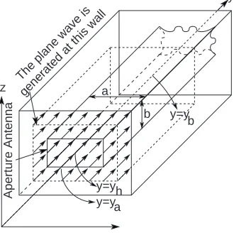
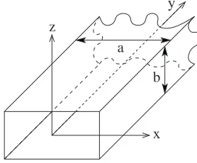
The complete geometry of a open-ended waveguide is shown in Fig. 2. The tangential electric field components along this structure are set to zero. Linearly polarized (alongz-axis) perfectly plane wave of Gaussian pulse propagating alongy-axis in free space incidents on the open end of the RW-90 waveguide as shown in the Fig. 1. The waveguide is extended up to last point of the PML to ensure that all the power entering into the waveguide is propagating through it to infinite and nothing will reflected back just acting like a match terminal.

y=ya

y=y b

y=yh

Aperture Antenna

generated at this wall

y

z The plane wave is

b a

Figure 1. Receiving antenna case. A open-ended waveguide under plane-wave illumination within the FDTD grid.

In order to simulate a uniform plane wave within the FDTD lattice, the problem space is divided into the total field and scattered field regains and the waveguide is placed within the total field regions. Details of this method given in [10], are used in this work. In [10] the plane wave is generated in the XZ-plane, at y = ya and subtracted

z

x b a

y

Figure 2. Front view of open-ended rectangular waveguide.

up to last point of PML and the EM wave propagates through the waveguide without any external disturbance and absorbed at the PML, the subtractions in the XZ-plane at y = yb take place like [10] but

without the area (a×b) inside the waveguide at y=yb.

As perfectly plane wave and lossless free space are considered, time domain electric field at the aperture of the open-ended waveguide is

Ezi,j,k(t) =Ae

−0.5

t−t₀₊t

tω

2

(3) where, t is the time shift due to the spacial difference between the antenna aperture and the position where Gaussian pulse is applied into the FDTD lattice. Fourier transform ofE_zi,j,kt gives the frequency domain incident electric field, which is

Ei(ω) =F{Ezi,j,k(t)} (4)

where, F{ }denotes the Fourier Transform. 2.2. Power Flowing through the Waveguide

The time average complex power flowing through the waveguide is given by [2, 12]:

Pc(ω) =

a

0

b

0

E(ω)×(H(ω))∗dx dz (5)

theXZ-plane (y=y0) ensures that the measuring device receives only the dominant mode scattered power. Neglecting all components except

Ez and Hx∗, time average power flowing through the waveguide along y-direction is real part of Pc(ω) which is given by:

Py(ω) ≈ Re{Pc(ω)}

≈ Re

a

0

b

0

[Ez(ω)×(Hx(ω))∗]y=y0dx dz (6)

where, y0 is the point in which all other modes are died down except

T E10 and minimum 3 cell before the P M Lstart in the FDTD space lattice.

2.3. Voltage Developed at the Matched Measuring Device

Since, most measuring devices have an input impedance of 50Ω, the voltage measured by these is given by:

VL(ω) =

50×Py(ω) Volts (7)

on the condition that the waveguide transporting this power is well matched with the measuring device.

2.4. Calculations of Far-field Antenna Factor

To carry out field strength measurements, one typically connects an antenna to a spectrum analyzer. The AF is the parameter that is used to convert the voltage or power reading of the receiver to the field strength incident on the antenna. In terms of an equation, the AF is defined as [13, 14]

AF = Ei(ω)

VL(ω)

m−1= 20log

Ei(ω) VL(ω)

dB

m−1

(8) where, Ei is the incident electric field on the surface of the antenna,

and VL, is the voltage induced across a 50Ω load of the receiver.

During the progress of the FDTD calculations the incident field

Ezi,j,k(t) and time domain electric fieldEz(t) and magnetic fieldHx(t)

AF of the antenna is evaluated using Eq. (8). FDTD predicted AF flowing through this procedure takes the account of mutual coupling effects [15].

For the numerical calculation, a programme developed in C using compiler gcc-4.0runs on a Pentium 3.0GHz processor based on personal computer supported by LINUX operating system.

3. NUMERICAL RESULTS & DISCUSSIONS

The complete geometry for a X-band waveguide of dimension a = 2.29 cm, b = 1.02 cm and c = 3λ corresponding to lowest frequency of operations 8 GHz, under consideration is shown in the Fig. 2. The tangential electric field components along this structure is set to zero. The simulations were carried out FDTD spacial grid with uniform cell size of x = y = z = 1.0mm (∼= λmin/24) where,

λmin = 24.0mm is the wavelength at the maximum frequency of 12.4 GHz. t is calculated from Eq. (1.11) of [10]. This fine spatial resolution permits direct modeling of the 1.0mm wall thickness of the metallic components, assumed to be PECs. A linearly polarized (alongz-axis) perfectly plane wave of Gaussian pulse having significant frequency content in a frequency range from 8 GHz to 12.5 GHz of maximum amplitude A = 1.0V/m given by the Eq. (1) incidence on the open end of the waveguide aty=yh. Other end of the waveguide

is extended up to last point of the PML to ensure that all the power entering into the open end of the waveguide is propagating through the waveguide to infinite and nothing will reflected back as it looks like a match terminal.

The experiment was carried out over the frequency range of 8 GHz to 12.6 GHz in steps of 0.2 GHz. The experimental apparatus and procedures are given in details in [2].

3.1. Open-ended Rectangular Waveguide Sensor

Empirical formula for computing AF ofx-band, W R-90waveguide, is given in [2], as

AF(dB) = 20log₁₀46.16f (9) It is the simplest formula for quick calculations of AF of an open-ended rectangular waveguide.

42 42.5 43 43.5 44 44.5 45 45.5

8 8.5 9 9.5 10 10.5 11 11.5 12 12.5

Antenna Factor (dB/m)

Frequency (GHz)

Empirical MoM FDTD Measurement

Figure 3. Variation of AF of a x-band open-ended rectangular waveguide sensor at normal incidence using FDTD, empirical formula, MoM [6] and experiment [6].

The experimental results show a better match with the FDTD formulation throughout the frequency band, compared to the empirical formula or MoM based analytical result [6] used by the EMC practitioners. The theoretical result using FDTD formulation starts showing significant variation from empirical formula after 10GHz onwards. As the empirical formula assumes only far-field type fields, the deviation from the empirical formula underlines the effect of non-far-field type fields at the sensing plane of the sensor. So, the present analysis becomes more and more useful beyond 10GHz.

The boundary conditions (PML) used in this work to truncate the FDTD lattice are not perfect [10], i.e., a certain portion of the wave reflects back from the PML to the waveguide and creates standing wave. For which unwanted sinusoidal variation of FDTD computed AF with respect to frequency is shown in the Fig. 3. However, this variation is also seen in the measurements, leading to the conclusion that it is an intrinsic antenna property.

3.2. Effects of Cross-polarizations

power flowing through the waveguide alongy-direction is changed by:

Py(ω)≈Re

a

0

b

0

[Ex(ω)×(Hz(ω))∗]y=y0dx dz (10)

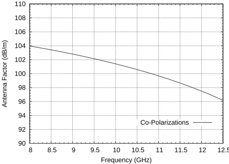
AF of open-ended waveguide is calculated in the same way shown in the Fig. 4. AF of the open-ended waveguide in this position is too much high. In practice the received power is too low to separate itself from the EMI noise present in the environment.

90 92 94 96 98 100 102 104 106 108 110

8 8.5 9 9.5 10 10.5 11 11.5 12 12.5

Antenna Factor (dB/m)

Frequency (GHz)

Co-Polarizations

Figure 4. Variation of AF with frequency of the cross-polarized (incident electric field orthogonal to the waveguide)x-band open-ended rectangular waveguide sensor at normal incidence.

3.3. Open-ended Rectangular Waveguide with Ground Plane

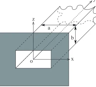
Use of a finite ground plane in measurements although the MoM theory in [2, 6] is for a sensor with infinite ground plane. The assumption of zero electric field throughout the ground plane except at the aperture opening, does not hold good when the ground plane is finite in extent. The motive for using short ground plane was to disturb the surrounding as little as possible. Further, the electromagnetic field scattered by structures behind the antenna may find a way into the open-end due to the presence of a finite ground plane. In this work AF of the open-ended waveguide is evaluated by adding a finite sized perfectly conducting ground plane of different size but multiple of (11 cm×10,cm) as reported in [16] on the open end of the waveguide at

z

x b

o a

y

Figure 5. Front view of open-ended rectangular waveguide with finite ground plane.

38 39 40 41 42 43 44 45 46 47 48

8 8.5 9 9.5 10 10.5 11 11.5 12 12.5

Antenna Factor (dB/m)

Frequency (GHz)

gp 2.5 cm X 2.27 cm gp 3.67 cm X 3.33 cm gp 5.5 cm X 5 cm gp 11.0 cm X 10 cm gp 22.0 cm X 20 cm gp 27.5 cm X 25 cm infinite gp without gp

Figure 6. Variation of AF with frequency for a x-band open-ended rectangular waveguide sensor with various sized finite ground plane (gp) at normal incidence.

ground plane is shown in the Fig. 6. A comparison is made between the AF of open-ended waveguide and open-ended waveguide with ground plane of different dimensions extended to infinite.

plane. The variation of AF for the ground plane of larger dimension 27.5 cm×25.0cm (7.33λmax×6.67λmax) for the wavelength λmax = 3.75 cm for the frequency 8 GHz, is much more than the smaller sized ground plane. The simulations of the ground plane larger than the size 27.5 cm×25.0cm with the same spacial resolution is not possible in our present hard-ware availability. So here the conclusion is that the ground plane size of (7.33λmax×6.67λmax) is not equivalent to the infinite ground plane when it is working in receiving mode which indicates something different from [2].

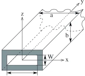
3.4. Rectangular Window Sensor

An electromagnetic wave incident on the window or the open-end of the waveguide causes an electric field to be induced at the plane of the window/open-end of the waveguide, which satisfies the boundary conditions imposed by the geometry of the waveguide. Detail study on the window radiator in receiving mod for EMI sensors using MoM is available in [2] and using Multiple Cavity Modeling Technique (MCMT) based on MON in [6]. Here in this work FDTD is used for the same analysis.

The open-ended waveguide receiver is the special case of the receiving window, when the window dimensions are the same as that of the waveguide, (xw,yw) refers to the center of the window with respect

to the center of the face of the receiving waveguide.

z

x a

b y

W

Figure 7. Front view of a window sensor.

43 43.5 44 44.5 45 45.5 46 46.5 47 47.5 48

8 8.5 9 9.5 10 10.5 11 11.5 12 12.5

Antenna Factor (dB/m)

Frequency (GHz)

MoM thick=0 mm MoM thick=1.6 mm FDTD Measurement

Figure 8. Variation of AF with frequency for a x-band rectangular window sensor of size L = 1.51 cm, W = 0.5 at normal incidence-FDTD, MoM [2] and experiment [2].

usable zone of the antenna factor is comparatively low. From Fig. 8 & 3, it is seen that the antenna factor of a window sensor is higher than that of the open end of a rectangular waveguide over the entire frequency range. FDTD computed AF is much closer to the experiment results than MoM in [2] because an infinite ground plane is considered in MoM analysis of [2] but in FDTD analysis need not to be considered any ground plane as experiment.

4. CONCLUSIONS

is also observed in the measurements leading to the conclusion that it is an intrinsic antenna property. This variation becomes more due to the dielectric insertion or in case of the use of the ground plane on the open face of the waveguide.

Again FDTD prediction of the antenna factor of EMI sensors is a very attractive alternative if one takes into consideration the enormous expenditure and time required for calibrating a sensor experimentally. Also, for experimental calibration, each and every sensor is to be calibrated individually, whereas for theoretical calibration all the sensors constituting a particular type can be calibrated at one go using the same approach; it is possible to predict the susceptibility of such antennas to electromagnetic radiation incident from any direction. Being time-domain technique, FDTD directly calculates the impulse response of an electromagnetic system. Therefore, a single FDTD simulation can provide either ultra wide band temporal waveforms or the sinusoidal steady state response at any frequency within the excitation spectrum. In case of FDTD, specifying a new structure to be modelled is reduced to a problem of mesh generation rather than the potentially complex reformulation of an integral equation. This technique can easily be extended to determine the antenna factor of any other types of antennas.

ACKNOWLEDGMENT

The author would like to thank Prof. A. Bhattacharya and Prof. A. Chakrabarty for critical discussion from time to time.

REFERENCES

1. Clayton, P. R., Introduction to Electromagnetic Compatibility, John Wiley & Sons Inc., New York, 1992.

2. Bhattacharya, A., S. Gupta, and A. Chakraborty, “Analysis of rectangular waveguide and thick windows as EMI sensors,”

Progress In Electromagnetics Research, PIER 22, 231–258, 1999. 3. Yu, W. and R. Mittra,Conformal Finite-Difference Time-Domain

Maxwell’s Equations Solver: Software and User’s Guide, Artech House, Boston, London, 2004.

5. Ali, M. and S. Sanyal, “A numerical investigation of finite ground planes and reector effects on monopole antenna factor,” Journal of Electromagnetic Waves and Applications, JEMWA, Vol. 21, No. 10, 1379–1392, 2007.

6. Das, S. and A. Chakrabarty, “A novel modeling technique to solve a class of rectangular waveguide based circuits and radiators,”

Progress In Electromagnetics Research, PIER 61, 231–252, 2006. 7. Sadiku, M. N. O.,Numerical Techniques in Electromagnetics, 2nd

ed., CRC Press, Boca Raton, London, New York, Washington, D.C., 2000.

8. Taflove, A. and S. C. Hagness, Computational Electromagnetic-The Finite-Difference Time-Domain Method, Artech House, Boston, London, 2005.

9. Bondeson, A., T. Rylander, and P. Ingelstrom, Computational Electromagnetics, 1st ed., Springer, New York, Oct. 2005.

10. Sullivan, D. M., Electromagnetic Simulation Using The FDTD Method, IEEE Press, New York, 2000.

11. Sullivan, D. M., “An unsplit step 3-D PML for use with the FDTD method,”IEEE Microwave Wireless Compon. Lett., Vol. 7, No. 7, 184–186, July 1997.

12. Harrington, R. F., Time-Harmonic Electromagnetic Fields, McGRAW-Hill Book Company, New York, 1961.

13. Iwasaki, T. and K. Tomizawa, “Systematic uncertainties of the complex antenna factor of a dipole antenna as determined by two methods,” Electromagnetic Compatibility, IEEE Transactions, Vol. 46, No. 2, 234–245, May 2004.

14. Joseph, W. and L. Martens, “An improved method to determine the antenna factor,” Instrumentation and Measurement, IEEE Transactions, Vol. 45, No. 1, 252–257, Feb. 2005.

15. Hekert, R. M., J. K. Daher, K. P. Ray, and B. Subbarao, “Measurement and modeling of near and far field antenna factor,”

International Conference on Electromagnetic Compatibility and Interference (INCEMIC’1994), 237–241, Aug. 1994.