Western University Western University
Scholarship@Western
Scholarship@Western
Electronic Thesis and Dissertation Repository
12-19-2018 11:00 AM
Partitioning and Offloading for IoT and Video Streaming
Partitioning and Offloading for IoT and Video Streaming
Applications that Utilize Computing Resources at the Network
Applications that Utilize Computing Resources at the Network
Edge
Edge
Navid Bayat
The University of Western Ontario
Supervisor Lutfiyya, Hanan
The University of Western Ontario Graduate Program in Computer Science
A thesis submitted in partial fulfillment of the requirements for the degree in Doctor of Philosophy
© Navid Bayat 2018
Follow this and additional works at: https://ir.lib.uwo.ca/etd
Part of the Computer Sciences Commons
Recommended Citation Recommended Citation
Bayat, Navid, "Partitioning and Offloading for IoT and Video Streaming Applications that Utilize Computing Resources at the Network Edge" (2018). Electronic Thesis and Dissertation Repository. 5937.
https://ir.lib.uwo.ca/etd/5937
This Dissertation/Thesis is brought to you for free and open access by Scholarship@Western. It has been accepted for inclusion in Electronic Thesis and Dissertation Repository by an authorized administrator of
Abstract
The Internet of Things (IoT) is a concept in which physical objects embedded with sen-sors, actuators, and network connectivity can communicate and react to their surroundings. IoT applications connect physical objects for the purpose of decision making by sensing and analysing generated data from the embeddedsensors in physical objects. IoT applications are growing rapidly as sensors become less expensive. Sensors generate large amounts of data that may meaningless unless the data is used to derive knowledge with in a certain period of time. Stream processing paradigm is used by IoT to provide requirements of IoT applications. In a stream processing paradigm, unlike traditional data bases, data is not stored but rather processed as it is generated. To transfer generated data from distributed data sources to a pro-cessing center such as cloud may not allow for real-time propro-cessing due to the network delay. Another high-demand application is live streaming of video. The performance of live video stream systems is inferior when there is a sudden large demand in the number of users. This thesis addresses some of the limitations of current architectures for video streaming systems and IoT applications based on the use of nearby computing resources (e.g., cloudlet, fog).
First, we addressed the degrading performance in video stream systems when a flash crowd occurs. The performance of video streaming systems is affected by flash crowd and degrade the quality of service for subscribers to the content delivery system. A flash crowd happens when there is a sudden large increase in the number of users. Therefore, flash crowds increase network traffic for any particular server. The main challenge is to make sure that the video streaming system has sufficient capacity to handle the occurrence of flash crowds.
Second, we address the limitation of current architectures for running mobile applications by introducing a dynamic partitioning and offloading of a mobile application. Mobile devices have limited resources including short battery life, storage capacity and processor performance. This limits the applications that can run on it. Mobile applications can be partitioned so that some of the application runs on a cloud. This works well for applications with relatively little data to be transferred and that do not have a high level of interaction with the user. Challenges with applications that have large amounts of data to be transferred and have a high level interac-tiveness is the high latency incurred by the network and packet loss of the wireless network. A mobile application can be partitioned so that part of it runs on a nearby computing resource e.g., fog node or cloudlet. This thesis presents a framework that introduces fine-grained offloading approach and support for runtime and dynamic partitioning of an application.
Third, we present a solution for placement of stream operators over distributed fog nodes for live processing of data streams from geographically distributed data sources. This place-ment of stream operators takes place in such a way that it supports applications with a high volume of data that require real-time (or near real-time) analysis To this end, this thesis pro-posed a set of algorithms for placement of stream operators among fog nodes.
Keywords: Internet of Thins, Data Streaming, Big Data, Context-aware, Query Graph, Fog Platform, Offloading, Partitioning.
Acknowlegements
Firstly, I would like to express my sincere gratitude to my advisor Professor Hanan Lutfiyya for her continuous support of my Ph.D study and my research, for her patience, and motivation. Her guidance helped me in all the time of my research and writing of my thesis. I could not have imagined having a better advisor for my Ph.D program. Last but not least, I would like to thank my parents and to my brother for supporting me spiritually throughout my Ph.D study and writing my thesis.
Contents
Abstract i
Acknowlegements ii
List of Figures vii
List of Tables ix
List of Appendices xi
1 Introduction 1
1.1 Internet of Things and Emerging Applications . . . 1
1.2 Characteristics of Emerging Applications . . . 2
1.3 Limitations of Current Architectures . . . 3
1.4 Thesis Focus . . . 3
1.4.1 Video Streaming Applications . . . 3
1.4.2 IoT Applications and Data Stream Processing . . . 4
1.5 Thesis Structure . . . 4
2 Background on Peer-to-Peer Networks 6 2.1 Peer-to-Peer Networks . . . 6
2.1.1 Classification of P2P Networks . . . 6
2.2 P2P Streaming Network . . . 7
2.2.1 P2P Live Streaming Systems . . . 7
2.3 P2P Network Topologies . . . 7
2.3.1 Tree-Based P2P Network for Live Video Streaming . . . 7
2.3.2 Mesh-based P2P Network for Live Streaming Network . . . 8
2.4 Gap Analysis . . . 8
3 Handling Flash Crowd in P2P Multi-Channel Live Video Streaming 9 3.1 Challenges . . . 9
3.2 Related Work . . . 10
3.2.1 Flash Crowd . . . 10
3.2.2 Unbalanced Resource Distribution Among Channels . . . 11
3.2.3 Incentive Mechanism . . . 11
3.2.4 Network Coding . . . 11
3.3 Decentralized approach to handling flash crowds . . . 12
3.3.1 Overlay Structure . . . 12
3.3.2 Bootstrap nodes . . . 13
3.3.3 Trackers . . . 14
3.3.4 Buffer-map . . . 16
3.3.5 Incentive Mechanism . . . 16
3.3.6 Performance Evaluation . . . 16
End-to-End Delay . . . 17
Playback Delay . . . 18
Distortion . . . 18
Link Stress . . . 19
Stretch . . . 20
3.4 Reducing Bandwidth Consumption . . . 20
3.4.1 Live Video Deployment Using Network Coding . . . 21
3.4.2 Performance Evaluation for ECFC . . . 23
End-to-End Delay . . . 23
Average Playback Delay . . . 24
Distortion . . . 25
3.5 Conclusion . . . 26
4 MC-SkyNet: Mobile-Cloud Dynamic Partitioning for Mobile Cloud Applications 27 4.1 Introduction . . . 27
4.2 Related Work . . . 28
4.2.1 Partitioning . . . 28
4.2.2 Offloading . . . 29
4.3 MC-Skynet Overview . . . 30
4.3.1 Partitioning . . . 31
4.3.2 Offloading . . . 32
4.3.3 Use of a Cloudlet Mesh . . . 33
4.4 Performance Evaluation . . . 34
4.4.1 Simulation Setup . . . 34
4.4.2 Evaluation . . . 35
Response Time . . . 35
Average Computation Cost . . . 35
Distortion . . . 36
Throughput . . . 37
Estimating the Time Constraint . . . 37
4.5 Conclusion . . . 39
5 Related Work on Data Stream Processing 40 5.1 Data Streaming Processing . . . 40
5.1.1 Classification of stream processing systems . . . 41
5.1.2 Representative Data Stream Processing Platforms . . . 41
5.2 Geo-Stream Management System (GSMS) . . . 43
5.2.1 Real-time Sensor Data Stream . . . 43
5.2.2 Sensor Data Stream Management Systems . . . 43
Hadoop-GIS . . . 44
Spatial and Spatio-Temporal Database Systems . . . 44
5.3 Query Operator Placement . . . 44
5.4 Gap Analysis . . . 45
6 Query Operator Problem Formulation 46 6.1 Reviewing the Impact of Using Fog Platform on IoT Applications . . . 46
6.2 Definition of a Query Graph . . . 47
6.3 Example Application Scenarios and Query Graphs . . . 47
6.3.1 Local Congested Highway Notification Scenario . . . 48
6.3.2 Local Camera Surveillance Scenario . . . 48
6.3.3 Regional Congestion Traffic Notification . . . 49
6.3.4 Regional Camera Crowd Size Measurement Scenario Results . . . 50
6.4 Query Plan Embedding . . . 51
6.4.1 Embedding Distortion Computation . . . 51
6.4.2 Cost of Embedding a Query Graph . . . 52
Impact of Weight Factorψin the Cost Function . . . 53
7 Study the Impact of Using Fog Platform on IoT Applications 54 7.1 Performance Metrics . . . 54
7.2 Experimental Environment . . . 55
7.3 Results of Local Congested Highway Notification . . . 55
7.4 Results of Local Crowd Size Measurement with Camera Surveillance . . . 56
7.5 Results of Regional Congestion Traffic Notification . . . 58
7.5.1 Experimental Configurations . . . 58
7.5.2 Results of Configuration 1, 2, 3, 4, 5, and 6 . . . 59
7.6 Results of Regional Camera Surveillance Scenario . . . 61
7.6.1 Experimental Configurations . . . 63
7.6.2 Results for Configuration 1, 2, 3, 4, 5, and 6 . . . 64
7.7 Conclusion . . . 71
8 Proposed Embedding Algorithms 72 8.1 Query Graph Reshaping Algorithms . . . 72
8.1.1 Reconfiguration Query Graph Algorithm . . . 72
8.1.2 Adjustment of Reconfigured Query Graph Algorithm . . . 75
8.2 Mapping Algorithm . . . 78
8.2.1 Proposed Mapping Algorithm . . . 78
9 Performance Evaluation 80 9.1 Configuring the Simulation Environment . . . 80
9.1.1 Fog Node Networks Used . . . 80
9.1.2 Applications . . . 81
9.1.3 Cost Functions for Mapping Algorithm . . . 81
9.2 Congested Highway Notification Scenario Results . . . 82
9.2.1 Average Execution Time . . . 82
9.2.2 Average End-to-End Delay . . . 83
9.2.3 Average Response Time . . . 85
9.2.4 Average Distortion Due to Buffering . . . 86
9.2.5 Average Distortion Due to Network Latency . . . 86
9.3 Camera Crowd Size Measurement Scenario Results . . . 87
9.3.1 Average Execution Time . . . 88
9.3.2 Average End-to-End Delay . . . 91
9.3.3 Average Response Time . . . 94
9.3.4 Average Distortion Due to Buffering . . . 96
9.3.5 Average Distortion Due to Network Latency . . . 100
10 Conclusion 103 10.1 Future Work . . . 104
Bibliography 105 A Simulator 122 A.1 Introduction to the Simulator . . . 122
A.1.1 Data Stream Processing in the Simulator . . . 123
A.2 iFogSim Extension . . . 124
A.2.1 Setting up Delay in the iFogSim . . . 124
End-to-End Calculation . . . 125
A.2.2 Gateway . . . 126
B Query Graph 131 B.1 Query Graph for Congested Highway Notification Scenario . . . 131
B.2 Camera Crowd Size Measurement Scenario . . . 135
Curriculum Vitae 138
List of Figures
3.1 Multi-Tree Construction for Sub-Streaming . . . 13
3.2 Average End-to-End Delay . . . 18
3.3 Average Playback Delay . . . 19
3.4 Average Distortion . . . 19
3.5 Average Link Stress . . . 20
3.6 Average Stretch . . . 21
3.7 General Network Coding Technology [43] . . . 22
3.8 Integration of the Sub-streaming and Network Coding Technology . . . 23
3.9 Average End-to-End Delay . . . 24
3.10 Packet forwarding without (a) and with network coding (b). . . 24
3.11 Average Playback Delay . . . 25
3.12 Average Distortion . . . 25
4.1 Framework . . . 30
4.2 Regression Tree Structure . . . 32
4.3 Average Response Time . . . 36
4.4 Average Execution Time . . . 36
4.5 Average Distortion . . . 37
4.6 Average Throughput . . . 38
5.1 Data Stream Management Systems classification [147] . . . 41
6.1 Query Graph for Local Traffic Congestion Notification Scenario . . . 48
6.2 Local Camera Crowd Size Scenario Query Graph . . . 49
6.3 Query Graph for Traffic Congestion Notification Scenario . . . 50
6.4 Camera Crowd Size Scenario Query Graph . . . 51
8.1 Camera Crows Size Scenario Query Graph . . . 73
8.2 Reconfigured Query Graph . . . 73
8.3 Adjusted Query Graph . . . 77
8.4 Example of a Query Graph . . . 78
A.1 Sequence diagram of the generation and execution [79] . . . 123
A.2 An Example of an Underlay Network . . . 124
A.3 An Example of an Underlay Adjecency Martrix . . . 125
A.4 Example of a Transmission Rate Matrix for an Underlay Network . . . 126
A.5 An Example of an End-to-End Delay [20] . . . 126
A.6 An Example of a Cloud and Fog Nodes . . . 127
A.7 An Example of Fog Node and Data Sources . . . 127
A.8 An Example of Fog Node and Data Sources with a Gateway . . . 128
A.9 (a) An Example of two entities in the Simulation, (b) An Example of Two entities with Physical Network Connection . . . 129
A.10 An Example of Five Fog Nodes in the Simulation . . . 130
A.11 An Example of Five Fog Nodes with Physical Network Connection . . . 130
B.1 Original Query Graph for Traffic Congestion Notification Scenario . . . 131
B.2 Camera Crowd Size Scenario Query Graph . . . 135
List of Tables
3.1 Simulation Parameters . . . 17
4.1 Simulation Parameters . . . 35
7.1 Average Execution Time . . . 55
7.2 Average End-to-End Delay . . . 56
7.3 Average Response Time . . . 56
7.4 Distortion Due to Buffering . . . 56
7.5 Distortion Due to Network Latency . . . 56
7.6 Average Execution Time . . . 57
7.7 Average End-to-End Delay . . . 57
7.8 Average Response Time . . . 58
7.9 Average Distortion Due to Buffering . . . 58
7.10 Average Distortion Due to Network Latency . . . 58
7.11 Maximum Mapping Distortion for Congested Highway Notification Scenario . 59 7.12 Average Execution Time-Configuration 1, 2, 3, 4, 5, and 6 . . . 60
7.13 Average End-to-End Delay-Configuration 1, 2, 3, 4, 5,and 6 . . . 61
7.14 Average Response Time-Configuration 1, 2, 3, 4, 5,and 6 . . . 62
7.15 Average Distortion Due to Buffering-Configuration 1, 2, 3, 4, 5,and 6 . . . 63
7.16 Average Distortion Due to Network Latency-Configuration 1, 2, 3, 4, 5,and 6 . 64 7.17 Maximum Mapping Distortion for Congested Highway Notification Scenario . 64 7.18 Average Execution Time-Configuration 1, 2, 3, 4, 5, and 6 . . . 66
7.19 Average End-to-End Delay-Configuration 1, 2, 3, 4, 5, and 6 . . . 67
7.20 Average Response Time-Configuration 1, 2, 3, 4, 5, and 6 . . . 68
7.21 Average Distortion Due to Buffering-Configuration 1, 2, 3, 4, 5, and 6 . . . 69
7.22 Average Distortion Due to Network Latency-Configuration 1, 2, 3, 4, 5, and 6 . 70 9.1 Maximum Embedding Distortion for Congested Highway Notification Scenario 82 9.2 Average Execution Time-1000 Vehicles . . . 83
9.3 Average Execution Time-2000 Vehicles . . . 83
9.4 Average End-to-End Delay-1000 Vehicles . . . 84
9.5 Average End-to-End Delay-2000 Vehicles . . . 84
9.6 Average Response Time-1000 Vehicles . . . 85
9.7 Average Response Time-2000 Vehicles . . . 86
9.8 Average Distortion Due to Buffering-1000 Vehicles . . . 87
9.9 Average Distortion Due to Buffering-2000 Vehicles . . . 87
9.10 Average Distortion Due to Network Latency-1000 Vehicles . . . 88
9.11 Average Distortion Due to Network Latency-2000 Vehicles . . . 88
9.12 Maximum Embedding Distortion for Camera Crowd Size Measurement Scenario 89 9.13 Average Execution Time-64 Cameras . . . 89
9.14 Average Execution Time-128 Cameras . . . 89
9.15 Average Execution Time-256 Cameras . . . 90
9.16 Average Execution Time-512 Cameras . . . 90
9.17 Average Execution Time-640 Cameras . . . 91
9.18 Average End-to-End Delay-64 Cameras . . . 92
9.19 Average End-to-End Delay-128 Cameras . . . 92
9.20 Average End-to-End Delay-256 Cameras . . . 93
9.21 Average End-to-End Delay-512 Cameras . . . 93
9.22 Average End-to-End Delay-640 Cameras . . . 94
9.23 Average Response Time-64 Cameras . . . 95
9.24 Average Response Time-128 Cameras . . . 95
9.25 Average Response Time-256 Cameras . . . 96
9.26 Average Response Time-512 Cameras . . . 96
9.27 Average Response Time-640 Cameras . . . 97
9.28 Average Distortion Due to Buffering-64 Cameras . . . 97
9.29 Average Distortion Due to Buffering-128 Cameras . . . 98
9.30 Average Distortion Due to Buffering-256 Cameras . . . 98
9.31 Average Distortion Due to Buffering-512 Cameras . . . 99
9.32 Average Distortion Due to Buffering-640 Cameras . . . 99
9.33 Average Distortion Due to Network Latency-64 Cameras . . . 100
9.34 Average Distortion Due to Network Latency-128 Cameras . . . 101
9.35 Average Distortion Due to Network Latency-256 Cameras . . . 101
9.36 Average Distortion Due to Network Latency-512 Cameras . . . 102
9.37 Average Distortion Due to Network Latency-640 Cameras . . . 102
List of Appendices
Appendix A Simulator . . . 122 Appendix B Query Graph . . . 131
Chapter 1
Introduction
Over the last decade, the cloud paradigm has been extensively adopted [159]. A recent survey [178] on the adoption rates of cloud computing by enterprises reported that 63% of enterprises are using the cloud. The reason for the success of the cloud paradigm is that it offers scalability, flexibility, and services on demand to customers [137][8]. For example, the cloud paradigm provides services that include infrastructure as a service, platform as a service, and software as a service [148]. There are a number of commercial cloud platforms that provide computing resources to their clients over the Internet such as Amazon Web Services and Microsoft Azure [54]. A key advantage to cloud computing is that computing resources for an application can be adjusted on demand to support fluctuating workloads and thus drive down costs for enterprises [8]. Many smartphone applications use the cloud to offload resource intensive computational tasks. For example, Apple’s Siri [151] performs computational intensive speech recognition in the cloud and returns the results to the user [81].
The rest of this chapter is organized as follows: Section 1.1 describes emerging trends in applications. Section 1.2 discusses the characteristics and requirements of Internet of Things (IoT) applications and real-time data-intensive applications. Limitations of current architec-tures for these applications is discussed in Section 1.3. The contribution of this thesis is ex-plained in Section 1.4. Section 1.5 provides the structure of the thesis.
1.1
Internet of Things and Emerging Applications
The Internet of Things (IoT) is a paradigm that envisions the physical world as a smart space in which physical objects are equipped with sensors, actuators, and network connectivity that can communicate and react to their surroundings [13]. Cisco estimates that there will be around 25 billion to 50 billion connected devices by 2020 [64]. A new generation of applications is emerging in which data is collected from the sensors embedded into physical objects. Several of these applications are described below [108]:
• Early Disaster Alerting: Sensors can collect crucial information about the environment and detect environmental disasters such as earthquakes and tsunami which help save lives.
• Health Care and Patients Surveillance: Constant monitoring of patients can save lives.
2 Chapter1. Introduction
For example, emergency care can be dispatched immediately when a patient begins to experience a heart attack.
• Smart Surveillance Camera: The use of smart surveillance cameras allow authorities to detect when crime has occurred and respond faster.
• Agricultural Efficiency: Soil moisture sensors and weather sensors can sense soil mois-ture and take weather information into account for smart irrigation systems. Smart ir-rigation systems only water crops when needed and thus reduce the amount of water usage.
• Smart Navigation Systems in Smart Cities: Consider a smart city where all the vehicles are equipped with a sensor that periodically emits a position report that identifies the vehicle’s location. The position reports can be used to determine congestion. If there is congestion, vehicles can be notified so that drivers can reroute.
• Smart Buildings: Consider a scenario where a sensor network is used to monitor the temperature of rooms in a building to sound an alarm in the case of a fire. This allows for for immediate and necessary fire detection [141]. Each temperature measurement report generated by any sensor in the building should be checked as soon as possible in order to detect a fire.
In the near future, the number of sensors are expected to grow exponentially and hence the increase in IoT applications (with real-time or near real-time requirements) [171].
In the past decade, not only have high data rate sensors such as video cameras become more pervasive, but the consumption of video contents have also changed from offline viewing to online streaming [153]. Furthermore, as portable devices with cameras have become more ubiquitous, users are able to create and share videos. Users are increasingly demanding content at any time of day, from any device and from any place. With these media streaming applica-tions, it is important that the user receives the media content in real-time. This is especially important for live events (e.g., sports events). For example, live streaming events such as video broadcasts from the Olympic Games can cause very high traffic due to a huge number of fans [185]. In addition, many security applications use video surveillance cameras to provide secu-rity. These security applications process the received video content from surveillance cameras to extract knowledge and deliver the results (suspicious activity) to the user(s) devices (e.g., smartphone) through the Internet [31].
1.2
Characteristics of Emerging Applications
1.3. Limitations ofCurrentArchitectures 3
1.3
Limitations of Current Architectures
Currently, IoT applications assume that sensor data is sent to a cloud for analysis and to de-termine a response. For example, a Fitbit offloads its data to an online account maintained by services hosted on a cloud. This works well for a Fitbit since real-time analysis and response is not essential. However, for security applications that use video surveillance this is not the case. The problem of relying solely on the cloud is the issue of latency. Latency is due to the network delay from the IoT devices to the cloud, which may often times lead to poor quality of service (QoS). Furthermore, the network core can become overwhelmed [111]. This makes the use of a cloud unsuitable for applications that require a high level of interaction with users and applications with real-time decision making requirements [77][115][44][78][162].
Video streaming applications make use of peer-to-peer networks where processing often makes use of computing resources close to data sources. This is done to address latency. However, much of the existing work suffers from overutilization or underutilization of geo-graphically distributed processing units due to lack of management information [78][162].
1.4
Thesis Focus
This thesis addresses some of the limitations of current architectures for video streaming and IoT applications by using nearby computing resources (e.g., cloudlet, fog). A cloudlet is de-fined as a resource-rich computer that is connected to the Internet and is available at the network edge for use by nearby end-devices (e.g., smartphones, tablets, vehicles) [82][165][154][98][23]. Fog (similar to a cloudlet) extends the cloud power to the edge of networks, in particular wire-less networks for the Internet of Things (IoT) [89][30]. Fog nodes are located away from the main cloud data centers (e.g., at any point from the data source to the cloud) [30]. Differences between cloudlet and fog are discussed in [58]. The rest of this section presents the thesis contributions.
1.4.1
Video Streaming Applications
Peer-to-Peer (P2P) networks consist of a set of nodes used to share access to data. P2P net-works provide a robust, reliable and scalable message routing and delivery on top of a physical (underlay) network. Large-scale commercial P2P streaming networks such as Coolstreaming [200] and PPLive [166] offer numerous video channels to thousands of users, simultaneously. These are referred to as multi-channel P2P streaming networks [186]. In these types of net-works, peers can participate in more than one channel and switch between them. This thesis addresses the following challenges:
• Imbalance of resource usage of different channels
4 Chapter1. Introduction
1.4.2
IoT Applications and Data Stream Processing
In IoT applications, data takes the form of data streams. A data stream is defined as an un-bounded sequence of tuples (stream elements) that is produced incrementally over time [76] [134]. A tuple is defined as an atomic data item embedded in a data stream and can be pro-cessed by a processing unit [55]. IoT applications can use queries to aggregate continuous data from data sources and process streams of data to produce the output [198][9]. In an IoT application, a query may run continuously. This type of query is referred to as continuous query [14]. A continuous query consists of one or more query operator(s) such as map, join, aggregate, filter and union. A query operator is a function which is used to process an input data stream and produce output results [83][157].
This thesis proposes an approach for placing query operators on fog nodes and the cloud. In this thesis, a query operator placement algorithm is proposed, which supports:
• Real-time aggregating and analysing data streams from different geographically dis-tributed data sources.
• Combining more operators into one query graph instead of having different query graphs for each operator helps to save bandwidth and reduce transmission costs.
• Optimized operator placement and operator reuse.
• Scalability for distributed data stream management systems.
1.5
Thesis Structure
The remainder of this thesis is organized as follows:
• Chapter 2: Chapter 2 discusses data stream processing for IoT applications background and peer-to-peer live video streaming systems.
• Chapter 3: Chapter 3 presents a novel framework for multi-channel P2P live video streaming that provides de-centralized mechanisms for handling flash crowds that in-cludes incentive mechanism, load balancing mechanisms, and cross-channel help among peers for live video streaming in multi-channel P2P systems.
• Chapter 4: Chapter 4 presents a dynamic partitioning strategy that considers network conditions and the amount of data being transferred, shows how a cloudlet mesh can be used, and presents performance results that illustrate the advantages of a dynamic partitioning strategy and a cloudlet mesh.
• Chapter 5: Chapter 5 presents related work for concepts of data streaming such as oper-ators and continuous queries.
1.5. ThesisStructure 5
• Chapter 7: Chapter 7 presents the results of experimental studies that compare the use of using one or more levels of fog nodes for high and low volumes of data. Also, this chapter explores the need for an approach that places query operators on fog nodes.
• Chapter 8: Chapter 8 presents the proposed algorithms for query operator placement among distributed fog nodes.
• Chapter 9: Chapter 9 presents simulation results of the algorithms proposed in Chapter 8. The main goal is to show how the proposed algorithms can improve response time.
Chapter 2
Background on Peer-to-Peer Networks
This chapter presents background knowledge on work related to peer-to-peer (P2P) networks and streaming of live video over P2P networks.
This chapter is organized as follows: Section 2.1 presents peer-to-peer concepts and seman-tics. Section 2.2 provides an overview of basic peer-to-peer data streaming systems. Section 2.3 presents peer-to-peer overlay network typologies. Section 2.4 discusses the limitations of current peer-to-peer live video streaming systems.
2.1
Peer-to-Peer Networks
Peer-to-Peer (P2P) networks consist of a set of nodes (peers) that share their available resources (e.g., upload and download bandwidth, computational resources, data storage resources). P2P networks provide a robust, reliable and scalable message routing and delivery on top of a physi-cal (underlay) network. Peer-to-Peer network applications such as video on demand, live video streaming, and file sharing have become popular due to their scalability [50]. Recent studies [185][195][42] have shown that the overall P2P traffic on the Internet has been constantly in-creasing and that more than 60% of Internet traffic is generated by P2P network applications .
2.1.1
Classification of P2P Networks
P2P networks can be classified into the following categories:
• Centralized P2P Networks: In a centralized P2P network, a set of servers maintain a database of available services. A newly joined peer in a centralized P2P network needs to submit a request for the resource (e.g., a file) to a server. The server then looks to find the list of peers that can provide the requested service e.g., the requested file.
• Decentralized P2P Networks: Unlike the centralized approach, in a decentralised P2P network, peers connect to other peers (neighbours) and share resources among each other without any centralized server. Each peer obtains a service by sending a request to all its neighbours. Two common types of decentralized P2P networks are unstructured and structured:
2.2. P2P StreamingNetwork 7
– Unstructured: In an unstructured P2P network, peers randomly establish a connec-tion to a set of peers. The main problem with unstructured P2P networks is that a peer has to search the entire network to find a resource. The result is more latency and overhead to find a particular piece of data.
– Structured: In a structured P2P network, the overlay is organized into a specific topology (e.g., tree-based P2P network and mesh-based P2P network) [109].
2.2
P2P Streaming Network
P2P networks have become a popular approach to provide live video and video-on-demand (VoD) services. Commercial P2P live streaming and video-on-demand networks, such as PPLive [166], PPStream [176], UUSee [19], have successfully supported large subscribers [200].
2.2.1
P2P Live Streaming Systems
A P2P live stream includes a continuous flow of video that is generated in real-time. In a P2P live streaming network, a live video is disseminated to all subscribers in real-time. The video playbacks on all users are synchronized (i.e., each peer watches almost the same position of the video). In a P2P live streaming system, peers can join an on-going live streaming session and start watching the stream from the time they joined.
Recently, a new breed of commercial P2P video streaming applications has emerged [200] [166][25]. Large-scale commercial Peer-to-Peer (P2P) networks such as Coolstreaming [200] and PPLive [166] are extensively used for live video streaming. In almost all of these P2P video streaming systems, multiple channels broadcast video to thousands of users, simultaneously [48].
2.3
P2P Network Topologies
This section discusses P2P network topologies.
2.3.1
Tree-Based P2P Network for Live Video Streaming
8 Chapter2. Background onPeer-to-PeerNetworks
2.3.2
Mesh-based P2P Network for Live Streaming Network
In mesh-based P2P live streaming networks, each peer exchanges resources (e.g., data) with its neighbours. The main advantage of mesh-based P2P live streaming networks over tree-based P2P live video streaming is that mesh-based P2P live streaming is robust against peer churn. In a mesh-based P2P live streaming, if a neighbour peer(s) of a peer leave the system, the peer can receive stream (or download the video) from the remaining neighbours.
2.4
Gap Analysis
Chapter 3
Handling Flash Crowd in P2P
Multi-Channel Live Video Streaming
The deployment of live video streaming applications has seen a large growth on the Internet [196]. P2P networks provide a robust, reliable and scalable message routing and delivery on top of a physical (underlay) network. Large-scale commercial P2P streaming networks such as Coolstreaming [200] and PPLive [166] offer many video channels to thousands of users, simultaneously. These are referred to as multi-channel P2P streaming networks [86]. In these types of networks, the peers can participate in more than one channel and switch between them. This chapter focuses on the following challenges: imbalance of resource usage and flash crowd.
The rest of this chapter is organized as follows: Section 3.1 describes the challenges of current architecture. Section 3.2 presents related work. The proposed framework is presented in Section 3.3 and 3.4.
3.1
Challenges
This section describes the following challenges:
• Imbalance of Resource Usage: One challenge with the use of multi-channel networks is an imbalance in resource (such as bandwidth) usage of different channels [86][40]. This implies that some channels have satisfactory streaming qualities since they have a surplus of resources, while other channels suffer from unsatisfactory streaming quality due to a lack of sufficient resources.
• Flash Crowd: A flash crowd occurs when a large number of peers attempt to join a popular channel. A flash crowd can result in high consumption of upload bandwidth of a P2P network and thus causes a decrease in Quality of Service (QoS). One result is the lag between choosing a video and actual playback (i.e., the startup delay is high).
• Limited Available Bandwidth in P2P System: In a P2P system, the available band-width is limited and constitutes a critical bottleneck for the deployment of large scale video streaming applications. There is a need for more effective use of existing band-width.
10 Chapter3. HandlingFlashCrowd inP2P Multi-ChannelLiveVideoStreaming
3.2
Related Work
This section presents previous work with regard to P2P multi-channel live video streaming networks.
3.2.1
Flash Crowd
Flash crowds occur frequently in P2P live streaming systems. The sudden arrival of numer-ous peers may consume the bandwidth of a P2P network, and decrease the QoS [114]. Ex-isting methods for reducing the startup delay of a peer can be categorized into three types [114][40][189]. First, newcomers prefer to receive those chunks of video which have already been obtained by most other peers in the network. The reason for this is that this often increases the number of potential sources of the video chunk. However, if many peers already have the video chunk, then the video chunk may be removed from the buffer. Second, newcomers re-quest video chunks sequentially, in order to ensure seamless playback. Therefore, the diversity among video chunks among peers that arrive in a short period of time is low. As a result, peers that are part of a flash crowd upload few video chunks among each other. Third, newcomers do not exchange their buffer-map [85], which indicates which video chunks currently exist in the player buffer of peer, until they obtain enough video chunks, to decrease the signalling over-head. Hence, before the peer announces its buffer-map, other peers do not know which chunks of video their neighbours have and cannot download from them.
From the scalability view of P2P live streaming networks, Chen et al. [186] showed that a P2P live streaming network with admission control under a flash crowd can increase its upload-ing capacity to support higher request rates. Liang et al. [112] used a branchupload-ing process model to examine the service capacity of BitTorrent-like file sharing systems during flash crowds.
Load balancing problem in P2P networks is recognized as an important factor when en-suring that peers are not overloaded when flash crowd phenomena occur. Load balancing approaches depend on the type of P2P architecture [170]. For structured P2P system, Raoet et al. [114] proposed a scheme in which migration of a virtual server takes place between a set of heavy nodes and a set of lightly-loaded nodes. However, it has a serious drawback since it uses a number of directories to store and update the load information of the light nodes in the system, which consumes a large amount of resources in the P2P system. In unstructured P2Ps (e.g., Gnutella), random peer selection is commonly adopted. For example, Chawathe et al. [86] proposed a load balancing scheme based on the use of a random walk. It tries to increase the probability of visiting a lightly-loaded peer by organizing the overlay in such a way that a peer with high capacity has a large number of adjacent peers. There is a need for a global view of the system concerned with the distribution of the node capacities.
3.2. RelatedWork 11
3.2.2
Unbalanced Resource Distribution Among Channels
Multi-channel design techniques can be classified into three groups [184]; (1) In the Naive Bandwidth Allocation (NBA) approach [45], a peer subscribes only to its watched channels, and dedicates its upload bandwidth to them; (2) In the Passive Channel-aware Bandwidth Al-location (PCA) [181], a peer joins only to its watched channels, and optimally dedicates its upload bandwidth to these channels; (3) With the Active Channel-aware Bandwidth Alloca-tion (ACA) approach, a peer joins not only to its watched channels, but also to several other channels as a supporter. The main idea behind ACA is to allow the channels with surplus up-load bandwidth to help those with deficit upup-load bandwidth since the upup-load bandwidth is an important resource that greatly influences the quality of live video. In ACA, a peer optimally allocates its upload bandwidth to the watched channels and unwatched channels.
The View-Upload-Decoupling (VUD) [187] is the state-of-the-art framework for multi-channel live video streaming. VUD provides cross-multi-channel resource sharing. In VUD, each peer is assigned to one or more channels as a supporter. Therefore, video distribution for unpopular channels is achieved by utilizing the bandwidth of supporters from other channels. However, it still suffers from upload bandwidth overhead and distribution swarm management cost [59]. Liang et al. [112] have proposed a partial decoupling strategy instead of complete decoupling for viewing and uploading of a peer in multiple channels. Some of the peers with rich upload bandwidth are assigned to help other channels.
None of the above work proposed a mechanism to handle the flash crowd phenomenon or provides incentives for peers to share their upload bandwidth [123][61].
3.2.3
Incentive Mechanism
Most incentive mechanisms proposed for P2P networks [199][146] are centralized. CFC pro-posed a decentralized incentive mechanism. This is done by allowing neighbouring nodes to disconnect from a peer that is not responsive to its requests. If nodeicategorizes node jas one that does not respond to requests or has not sent a message then nodeidisconnects from node
j. If node j does not respond because it does not want to share its resources then nodeiwill not respond to node j’s requests. If a peer node is disconnected then it cannot receive video. This mechanism has elements of both encouragement and penalty schemes [146].
3.2.4
Network Coding
12 Chapter3. HandlingFlashCrowd inP2P Multi-ChannelLiveVideoStreaming
to significantly decrease the repair bandwidth. In [182], the author proposed a P2P storage cloud for on-demand streaming.
3.3
Decentralized approach to handling flash crowds
This section presents the Coping Flash Crowd (CFC) framework [22], that represents a decen-tralized approach to handling flash crowds. This is handled with the run-time construction of a hybrid mesh-tree overlay structure at the release time of a video and adapted when needed (e.g., for peer-churn and, support load balancing). To support resource sharing an incentive mechanism is proposed that encourages peers to allocate their upload bandwidth to other chan-nels. Since the quality of video at the peer side is related to its upload rate, it is very important to implement an incentive scheme for better streaming services. Without this mechanism, the flash crowd handling technique does not provide any advantages for reducing startup lag for peers.
3.3.1
Overlay Structure
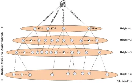
The use of a single tree structure for delivering video requires a root node, which is the video source. A peer only has one parent and a video stream is sent through each path. One of the disadvantages of a single tree is that the upload bandwidth of a leaf node is not utilized. This is addressed in a multi-tree where the video source divides the stream into multiple sub-streams. There is a sub-tree for each sub-stream. A leaf peer can be an internal node of another tree. One major drawback of tree-based streaming systems is their vulnerability to peer churn. A peer departure will temporarily disrupt video delivery to all peers in the sub-tree rooted at the departed peer. In a mesh-based structure, peers dynamically connect to a subset of random peers in the system. A peer pulls video content from its neighbors who have already obtained the content. Since multiple neighbors are maintained at any given moment, mesh-based systems are robust to peer churns. However, different data packets may traverse different routes to a peer. The arrival of data packets is unpredictable and thus peers may observe video playback quality degradation that includes long startup delays, frequent playback freezes and low video bit rates.
CFC uses a multi-tree but each peer dynamically connects to a subset of peers to form a mesh. Each tree in the multi-tree is responsible for a sub-stream but the mesh allows a node to receive other sub-streams. This reduces the time to receive video content, and to handle the peer churn. This combination of a multi-tree and mesh provides a pyramid-like overlay structure.
The video source uses the following formula to assign a sub-stream: i = GOPj mod k,
where k is the number of sub-streams andGOPj represents the jth Group of Picture (GOP).
3.3. Decentralized approach to handling flash crowds 13
types of peers and protocols needed to create and maintain the overlay are described in this section. These were designed to support load balancing and flash crowds.
Figure 3.1: Multi-Tree Construction for Sub-Streaming
3.3.2
Bootstrap nodes
Bootstrapping is the process by which a new peer joins the overlay structure. The goal of the bootstrapping operation is to find a node that is already a member of the overlay for it to connect to. This requires the use ofstretch information. For two nodes iand j, Di j is the number of
overlay hops between two nodes in the overlay network and the number of IP path hops is represented bydi j. The stretch factor is defined asS Ti j =
Di j
di j. The stretch factor represents the
overlay and underlay network mismatching (i.e., it represents the difference in the lengths of the shortest route between two nodes in the overlay and the shortest route between these nodes in the underlay network). For a nodeiand a set of nodes in setJ theaverage stretch valuecan be calculated as seen in Equation 3.1:
Avgstretch=
P|J|
j=1S Ti j
ω (3.1)
whereω= BWupload
AvgV BR andBWuploadis the average upload bandwidth the peers in setJ, andAvgV BR
is the average video bit rate of nodes in J.
TheGlobal Delay Stretchis the average stretch factor wheniis the video source andJis the
14 Chapter3. HandlingFlashCrowd inP2P Multi-ChannelLiveVideoStreaming
and J is the set of its children. This value changes as children are added. A set of peers are designated as bootstrap peers. A bootstrap peer is the root of a sub-tree, which is associated with a sub-stream. Each bootstrap peer directly receives its sub-stream from the video source. Each bootstrap peer keeps for each nodeiin its subtree the global delay stretch and available upload time. A newly arrived peer sends a request to the video source for a list of bootstrap nodes. The new peer randomly selects a bootstrap node and requests a joining point (a peer node that it may become the child of). IfAis the possible set of joining points then the joining point select is a node that with the addition of the newly arrived peers results in the smallest local delay stretch and the number of children associated with nodeihas not exceeded nodei’s limit. If there is no joining point the new peer will continue to contact bootstrap nodes until it finds a joining point. If no joining point is found, the new peer sends a message to the video source. The video source creates a new sub-stream.
The number of children that a nodeimay have is determined by the size of the sub-stream and the upload bandwidth of the node. The size of node i’s sub-stream is denoted by Si and
is between between Smin and Smax, where Smin is equal to the size of each GOP and Smax is
the length of the video stream. We assume that video has a variable bit rate which implies thatSmin andSmaxchanges. If BWiuis the upload bandwidth of peeriin the multi-tree overlay
network, the number of children for peer iin multi-tree isCi = BWu
i
Si where BWu
i
Smin ≤ Ci ≤ BWu
i Smax.
This calculation provides good QoS by not allowing an excessive number of peers to consume the upload bandwidth. If there areN peers let C be the min(Ci |0≤i≤ N−1).
Assume that the number of sub-streams ish. The number of peers at level 2 (height 2) and level 3 (height 3) ish×Candh×C×Crespectively. The number of peers of peers at leveliis
heighti=h×Ci. The minimal number (worse case) of peers in the tree is calculated as follows:
h
X
i
heighti=h∗ ×(C+C2+...+Ch−1)=h×(
1−Ch
1−C) (3.2)
When a sub-stream is created each peer in the multi-tree is able to accept at least one more child. The reason for this is that the number of GOPs becomes less. This allows for accommodation of flash crowds. The child nodes of a bootstrap node are designated asshadow
or backup nodes. The bootstrap peer for the new sub-stream is chosen from a set of backup
peers. When a bootstrap node leaves, a shadow node is chosen to replace it. This mitigates the effects of peer churn.
3.3.3
Trackers
Tracker peers, which are a subset of peers, are used to discover possible mesh neighbours for newly arrived peers. To support a node joining a mesh requires the use of tracker peers. Each tracker maintains a node-handle list and is referred to as a Local Tracker (LT). A node-handle list maintains information for a set of peers. Each peer in the node-handle list is a distance of
3.3. Decentralized approach to handling flash crowds 15
If the peer does not receive a message, it can then conclude that there are no available trackers within distancer. Therefore, the peer registers itself with the video source as a tracker. If the peer receives one or more responses to its ping messages, then the peer calculates the underlay distance between itself and the responding trackers. The requesting peer registers itself with the nearest tracker and requests a list of the active peers in the LTs node-handle list. Upon registration, the local tracker adds the registering peer to its node-handle list.
When a peer receives a list of neighbours it selects a set of neighbours for its mesh. This work uses physical network locality where choices are based on minimizing the traffic between the peer and selected neighbours. This is done by calculating the amount of traffic for the set of links, connecting the peer and a possible neighbour. The amount of trafficT(ta,tb)for sampling
time (ta,tb) for each underlay link,iis calculated as follows:
T(ta,tb)=
Ztb ta
linki(t) dt (3.3)
By approximating the average number of links and routers in the underlay network between two peers it is possible to estimate the average load on those links. To find the average number of routers between two peers we need to find the shortest path between two random selected nodes in the graph. The work described in [49] [103] [142] shows that for any graph the shortest distance is approximately:
d=ln[(N−1)( ˆZ2−Zˆ1)+Zˆ1
2 ]−ln( ˆZ1
2 ) ln( ˆZ2
2 /Zˆ1
2 )
(3.4)
where ˆZ1 is the average number of khop neighbours and N is the total number of vertices in
graph which are considered as routers. ˆZ1 and ˆZ2are defined as:
ˆ
Z1= [PN
x,y=1Axy]
N (3.5)
ˆ
Z2= [PN
x,y=1,x,yIAˆ(x,y)]
N (3.6)
In above equation theAis the routing adjacency matrix, and ˆAis equal toA2, andIis define
as:
IAˆ(x,y)={ 1, i fAˆxy>0
0, otherwise (3.7)
The traffic between two peers Aand B is based on the set of links connecting these two peers.
D= B
X
i=A
linki (3.8)
Therefore the average traffic on the underlay network isD×T(ta,tb). The lower the value of
16 Chapter3. HandlingFlashCrowd inP2P Multi-ChannelLiveVideoStreaming
3.3.4
Bu
ff
er-map
A peer’s buffer-map indicates which video chunks currently exist in the player buffer of a peer. Most buffer-maps consists of a zero or one representing the availability of a frame in the buffer of the peer. CFC proposes a new type of buffer-map structure to enhance video quality by reducing the end-to-end delay. This buffer-map includes four types of information: 1) Availability of the frames in the buffer; 2) Size of each frame in the buffer: 3) Estimation of response time; and 4) Average amount of free upload bandwidth.
By utilizing the buffer-map, peers estimate the time difference between the current time and the deadline of a chunk which we refer to as the urgent factor. A peer selects one of its neighbours to request a video chunk based on the urgent factor. We assume that a video chunk consists oflframes divided intocchunks, and f represents the frame rate of video (frames per second). Therefore, each chunk has the cf seconds of video. Moreover, the playback time of
n-th chunk can be computed as (n−1)lf. Let Sn be the size (measured in kilobytes) ofn-th
chunk, and Ti j be the transmission time between two peers i and j, and BWiu is the upload
bandwidth of peeri. Then-th chunk should be delivered within the amount of time represented byTi j +
Sn BWu
i
≤ (n−1)lf. Equ. 3.9 shows that the average busy time for each neighbour of a peer.
Tavg=
(1−γ)Tavg+γT
2 (3.9)
where Tavg is the average response time of that neighbor, γ is a coefficient for controlling
the effect of sudden changes of video rate. This means that when the video bit rate changes suddenly, the impact of video bit rate change should not affect the Tavg (refers to Equ. 3.9)
[24]. The average response time is depended on the free upload bandwidth capacity of peer’s neighbors. When video bit rate increases, it consumes more capacity of upload bandwidth of the peers to respond the video request message, and T is the necessary time to respond to a request by that neighbor in the last buffer-map exchange. We defineT as follows:
T= Si BWu
i + Sj
BWdj +Ti j (3.10)
WhereBWd
i is the download bandwidth of peeri.
3.3.5
Incentive Mechanism
Since the quality of video at the peer side is related to its upload rate, it is important to im-plement an incentive mechanism for live video streaming. Free riders in the P2P networks are peers that only use services but provide little or nothing in return. Therefore, it is important to encourage the peers to act as supporters and allocate their upload bandwidth for other channels.
3.3.6
Performance Evaluation
3.3. Decentralized approach to handling flash crowds 17
general, OverSim prepares a reusable framework that has two main parts; (1) Overlay layer: for creating neighbor relation and constructing the mesh (tree or structured systems), and (2) Application layer.
In this simulation, the underlay topology is generated by using the Georgia Tech Internet Topology Model (GT-ITM) [34] tools for OMNeT++v.4. This network is a decentralized and unstructured P2P network with 28 backbone routers, 748 access routers and 2000 peers. Peers in overlay network randomly select a router and connect to them by selecting random underlay link with a bandwidth between 128 Kbps to 2 Mbps and delays between 15 ms to 156 ms. In this simulation, video trace files are used from the Video Trace Library in [156] for streaming actual video. Table 3.1 shows the simulation parameters. In order to conduct a simulation that is more similar to the real world we generate the Constant Bit Rate (CBR) in the physical network. In order to load the network, it was imperative to set CBR background traffic to vary network load and enable us to study the proposed approach under different conditions. CBR traffic has been setup from various sources, with a 512 byte packet size. This background traffic operates during the entire duration of the simulations.
Table 3.1: Simulation Parameters
Simulation Parameters Value
Video Codec MPEG4
Video FPS 25
Number of Frame in GOP 12 Frames Selected Trace File Star Wars IV
Peer Upload Bandwidth Random(128,2048) Kbps Peer Download Bandwidth Random(512,2048) Kbps Average Video Bit Rate 512 Kbps
LifeTimeChurn Weibull Distribution Physical Link Delay Random(9, 156) ms Number of Channels 4
For peer churn, two different configurations are considered: (1) LifeTimeChurn. (2) NoChurn. In LifeTimeChurn configuration, when a peer is created, its life time is set randomly from the given probability function. When this life time is reached, the peer is removed from the net-work and a new peer will be generated. In Nochurn configuration, peers will be added until the target OverlayTerminalNum (the number of peers in the network) is reached and peers do not leave the network until the end of simulation. The focus on this work is not on scheduling algorithms and so a simple scheduling algorithm is used, similar to that proposed in [161]. The proposed framework is compared with View Upload Decoupling (VUD) which represents the state-of-the-art mechanism for multi-channel P2P systems.
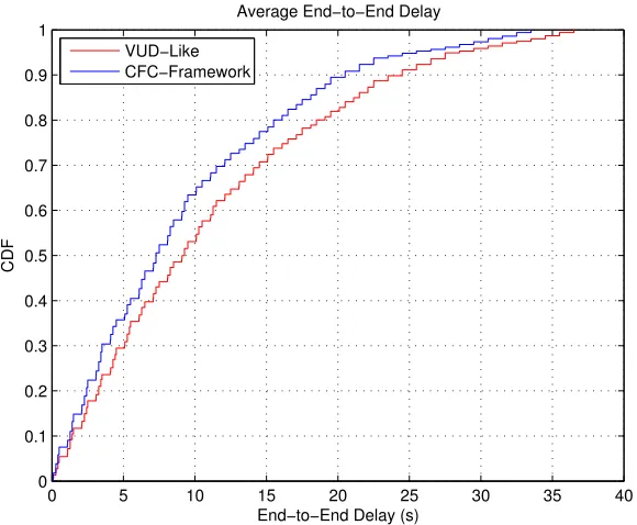
End-to-End Delay
The average end-to-end delay is defined as the average time between transmission and arrival of data packets from source to destination. The end-to-end delay is impacted by the average length of paths from the video source to the peers and the network diameter.
18 Chapter3. HandlingFlashCrowd inP2P Multi-ChannelLiveVideoStreaming
average end-to-end delay that is less than or equal toxseconds. For example, in Fig. 3.2, 50% of the peers have an average end-to-end delay that is less than 7 seconds but in the VUD-like implementation, 50% of the peers have an average end-to-end delay of less than 10 seconds. This represents a significant difference in playing time and shows the approach to neighbour selection (selection is based on physical network locality). It also shows that the incentive mechanism used by CFC is effective but VUD is not.
0 5 10 15 20 25 30 35 40
0 0.1 0.2 0.3 0.4 0.5 0.6 0.7 0.8 0.9 1
End−to−End Delay (s)
CDF
Average End−to−End Delay
VUD−Like CFC−Framework
Figure 3.2: Average End-to-End Delay
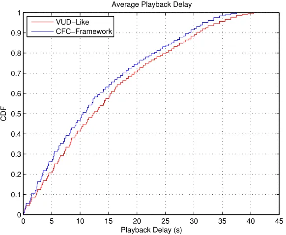
Playback Delay
Playback delay (start-up latency) in live video streaming is the difference of video timestamps between starting transmission time in the source node and playing time in the destination peer. It shows the time taken to fill the player buffer of the peers by considering the startup buffering time. The value of this metric increases as the size of the network grows. Fig. 3.3 shows similar results to Fig. 3.2 and thus provides further evidence of the effectiveness of the mechanisms introduced for CFC that are not found in VUD.
Distortion
Distortion (or video packet miss ratio) is a performance metric which shows the percentage of video content that is lost compared to the original video. Equ. 3.11 shows how distortion is calculated. The distortion rate consists of two parts: (1) Packet loss due to loss in the underlay links; and (2) Loss from frame play timeout. Fig. 3.4 provides further evidence that the mechanisms introduced for CFC are effective.
Distortion=(Total Size of Received Frames)×100
3.3. Decentralized approach to handling flash crowds 19
0 5 10 15 20 25 30 35 40 45
0 0.1 0.2 0.3 0.4 0.5 0.6 0.7 0.8 0.9 1
Playback Delay (s)
CDF
Average Playback Delay
VUD−Like CFC−Framework
Figure 3.3: Average Playback Delay
0 2 4 6 8 10 12 14 16 18 20
0 0.1 0.2 0.3 0.4 0.5 0.6 0.7 0.8 0.9 1
Distortion (%)
CDF
Average Distortion
VUD−Like CFC−Framework
Figure 3.4: Average Distortion
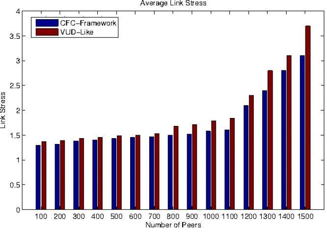
Link Stress
20 Chapter3. HandlingFlashCrowd inP2P Multi-ChannelLiveVideoStreaming
that only one packet enters into an AS, and all peers in that AS receive that packet. The max-imum number of link stress is N which is the number of peers in the AS. As Fig. 3.5 shows, redundant traffic can be safely reduced by considering the underlay hop count in neighbour selection. In CFC, peers select their neighbours by using dual-mode locality awareness, and implicitly considering the underlay distance between themselves and other peers in the net-work. As a result, they establish the connection with those peers with shorter distance in the underlay. It is known that peers in the same AS have shorter distances in underlay network. Therefore, neighbour selection inside the AS, instead of across AS, can reduce the link stress. It is noticeable that time is a critical factor for live video streaming. Therefore, video frames should be delivered to the destination before their playback time.
Figure 3.5: Average Link Stress
Stretch
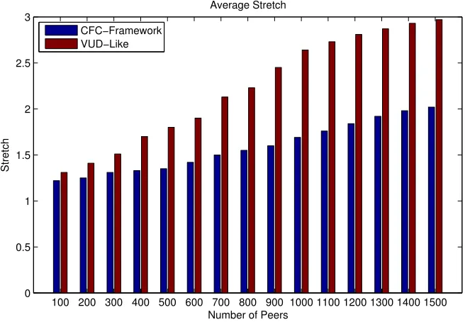
A lower stretch results in a better query time and reduces unnecessary bandwidth consumption [123]. Fig. 3.6 shows that the CFC reduces the stretch factor in the P2P network since it considers the stretch factor in selecting is neighbours for the mesh. This allows for a reduction in both the number of underlay and overlay hop counts.
3.4
Reducing Bandwidth Consumption
3.4. ReducingBandwidthConsumption 21
100 200 300 400 500 600 700 800 900 1000 1100 1200 1300 1400 1500 0
0.5 1 1.5 2 2.5 3
Number of Peers
Stretch
Average Stretch
CFC−Framework VUD−Like
Figure 3.6: Average Stretch
in the literature and used in P2P streaming networks (e.g., [186][187][188][112]). This work includes handling flash crowds but most of the work assumes the use of a central management node. To see the problems with the use of a central management node, consider a scenario such as a hockey or soccer game where fans want to share their video. In this scenario the identi-fication of a single management node that is persistent through the game may be difficult to identify. Load balancing techniques are often inadequate since peers are not always motivated to act as a supporter for other channels (intra-channel and cross-channel bandwidth allocation). To more efficiently use bandwidth, network coding was introduced [196].
3.4.1
Live Video Deployment Using Network Coding
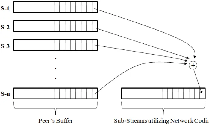
Assume that a peer wants to send a stream of video to its neighbours. To increase the through-put, the peer first divides a video stream intondifferent chunks. The peers can then exchange their chunks among their neighbours. Since a peer downloads pieces of the video from its neighbours simultaneously, the time for a peer to recover allnchunks of the packets is poten-tially much shorter than that of downloading the file from only a single peer. Figure 3.7 shows the concept of network coding [132] in the framework.
Figure 3.8 shows how each peer in the framework utilizes the power of network coding technology to push sub-streams which are in its buffer to its neighbours. S1, S2, S3, . . .,Sn
are the input sub-streams to the peer’s buffer. In this case, by using network coding technique each peer [132] encodes output sub-streams as a linear combination of the input sub-streams. In particular, assume that ai, andbi are new packets by linearly combining 4 chunks found in
buffer of peers AandBrespectively. Therefore,ai = P4j=1 f
a
i jcj, bi =
P5
i=2 f
b
i jcj, where f a i j and
fb
i j are random elements belonging to a finite field FQ [131], andc1,c2,c3,c4, ...are the video
22 Chapter3. HandlingFlashCrowd inP2P Multi-ChannelLiveVideoStreaming
Figure 3.7:General Network Coding Technology [43]
of peer C. Peer C downloads a1 = f11ac1 + f12ac2 + f13ac3 anda2 = f21Ac1+ f22ac2+ f23ac3 from
A and b1 = f12ac2+ fa13c3+ fa14c4 and b2 = f22bc2 + f23bc3 + f24bc4 from B. Peer C will be
able to reconstructc1,c2,c3,c4 if fi ja and f b
i j are known. Also, information about f a i j and f
b i j can
be included in the data packets. The number of bits required to specify fi ja and fi jbarenlog(q) wherenis the number of original packets whileqis the size of the finite field. Ifm>>nthen these bits are negligible. Therefore, for most practical purposes, this network coding scheme can speed up the download time. However, in this type of network coding some of the packets received at a peer may be duplicate, and thus resulting in wasteful bandwidth.
Assume that the overlay network is a graph of vertexes and edges. Each vertex in this graph is a representation of a peer in the network and each edge represents the connection between neighbours. If node A has c incoming edges {e1,e2, ..,ec} and one of the outgoing
edges ise, then the edge function of edgeein a linear network coding scheme can be denoted by a vector Vei = {fi jei}. The message on edge e is generated by the linear function Me =
fe1
1jMe1+f e2
2jMe2+f e3
3jMe3+...+f ec
c jMec, where Meirepresents the message transmitted on edge
ei [47] [182].
In this framework, if a source has capacityk, the source can transmit sub-streamsk simul-taneously. If the k sub-streams are represented by a k dimensional vector M, the messages transmitted over edgee can be represented by the product of vector M and anotherk dimen-sional vectorVe0. VectorV
0
eis called the edge vector of edgee. Therefore, the source generates
3.4. ReducingBandwidthConsumption 23
Figure 3.8: Integration of the Sub-streaming and Network Coding Technology
3.4.2
Performance Evaluation for ECFC
This section discusses the simulation results after incorporating network coding.
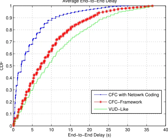
End-to-End Delay
In Fig. 3.9, the x-axis represents the average end-to-end delay and the y-axis represents values of the cumulative distribution function (CDF). A point (x,y) represents that y percentage of peers that have an average end-to-end delay that is less than or equal toxseconds. For example, Fig. 3.9 shows that 50% of the peers have an average end-to-end delay that is less than 7 seconds but in the VUD-like implemention we see that 50% of the peers have an average end-to-end delay of less than 10 seconds. This represents a significant difference in playing time. This shows that the approach to neighbour selection by CFC is effective compared to VUD. Fig. 3.9 shows a comparison of the end-to-end delay for CFC and ECFC. In ECFC peers try to establish a connection in the overlay tree as close as possible to the video source. To do so, they need to dedicate more resources to the network. This means that if any peer supports more peers in the network by uploading more video content, it can establish a connection to the higher levels of the tree. Accordingly, it will obtain the video packets in less time.
The comparison of CFC and ECFC shows the effectiveness of network coding in reducing the end-to-end delay. The network coding method combines received packets using a simple XoR operation as depicted in Fig 3.10(b). Peer P3 performs one less transmission using net-work coding which results in higher netnet-work throughput. PeerP3 in Fig 3.10.a needs to send both packets ”b1” and ”b2”, but in Fig 3.10.b, by using a network coding, peerP3 only sends
one packet (e.g,. b1⊕b2). Accordingly, peers P5 and P6 receive requested packets ”b1” and
”b2” with a lower end-to-end delay. The explanation is that the network coding reduces the
24 Chapter3. HandlingFlashCrowd inP2P Multi-ChannelLiveVideoStreaming
0 5 10 15 20 25 30 35 40
0 0.1 0.2 0.3 0.4 0.5 0.6 0.7 0.8 0.9 1
End−to−End Delay (s)
CDF
Average End−to−End Delay
CFC with Netowrk Coding
CFC−Framework VUD−Like
Figure 3.9: Average End-to-End Delay
Figure 3.10:Packet forwarding without (a) and with network coding (b)
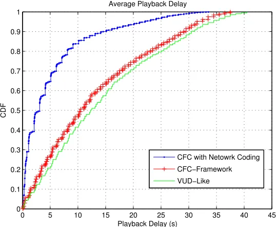
Average Playback Delay
3.4. ReducingBandwidthConsumption 25
0 5 10 15 20 25 30 35 40 45
0 0.1 0.2 0.3 0.4 0.5 0.6 0.7 0.8 0.9 1
Playback Delay (s)
CDF
Average Playback Delay
CFC with Netowrk Coding
CFC−Framework
VUD−Like
Figure 3.11: Average Playback Delay
Distortion
The distortion rate is impacted by the following: (1) Packet loss due to the loss in the underlay links; and (2) Loss from frame play timeout.
0 2 4 6 8 10 12 14 16 18 20
0 0.1 0.2 0.3 0.4 0.5 0.6 0.7 0.8 0.9 1
Distortion (%)
CDF
Average Distortion
CFC with Netowrk Coding
CFC−Framework
VUD−Like
26 Chapter3. HandlingFlashCrowd inP2P Multi-ChannelLiveVideoStreaming
3.5
Conclusion
This section summarizes the conclusions for CFC and EFC.
CFC is the first multi-channel P2P live video streaming architecture that considers mech-anisms for coping with the flash crowd phenomena alongside the load balancing, incentive mechanisms and traffic localization. Moreover, CFC proposed an incentive mechanism that encourages peers to share their upload bandwidth between different channels. The perfor-mance evaluation results demonstrated that CFC can decrease the redundant traffic between ASs. In CFC, even though peers do not have rich resources, upload and download bandwidth could also contribute to the system. It can cope the flash crowd phenomena in P2P Network, and reduce the start-up delay because in live video stream networks, a new comer expected to watch a video immediately. Some of the critical factors that are considered in CFC design that help mitigate the flash crowd phenomena include: (i) underlay and overlay load balancing; (ii) incentive mechanism; (iii) traffic localization.
Chapter 4
MC-SkyNet: Mobile-Cloud Dynamic
Partitioning for Mobile Cloud
Applications
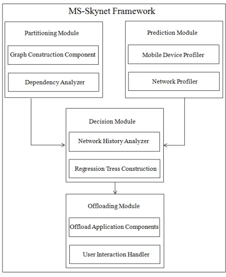
Mobile devices have limited resources including short battery life, storage capacity and pro-cessor performance. This limits the applications that can run on it. A mobile application can be partitioned so that some parts of the application runs on a cloud. This works well for applica-tions with relatively little data to be transferred and that do not have a high level of interaction with the user. High latency is a challenge with applications that have large amounts of data to be transferred with a high level interactiveness. A cloudlet is a resource-rich computer or cluster of computers that is connected to the Internet and is available for use by nearby mobile devices. A mobile application can be partitioned so that part of it runs on the cloudlet. This work presents the MC-Skynet framework which introduces fine-grained offloading approach and support for runtime and dynamic partitioning of a mobile application. This is different from previous approaches, in that MC-Skynet does not only provides dynamic partitioning and offloading, but is also adaptive to the changes of the state of a cloudlet. It does this by in-troducing a cloudlet mesh network and self learning decision making module to estimate the offloading cost.
4.1
Introduction
Mobile device applications either entirely run on mobile devices or computation is split be-tween the mobile device and a remote service. The remote service provides a well-defined API that can be used by mobile device applications (e.g., weather applications can use a remote ser-vice that collects weather data that becomes available through a well-defined API). The remote service may be hosted on a cloud. Regardless of the network distance between the cloud in-frastructure and the mobile device, the use of a remote service is well suited for mobile device applications with relatively little data to be transferred. However, long network distances be-tween mobile devices and remote services makes this approach unsuitable for applications that require larger amounts of data to be transferred and/or have a high level of interaction with the user. This includes mobile video communications (e.g., Skype, Face-Time, Google-Hangout),
![Figure 3.7: General Network Coding Technology [43]](https://thumb-us.123doks.com/thumbv2/123dok_us/1915287.1251207/34.612.119.477.71.332/figure-general-network-coding-technology.webp)