Analysis of Electromagnetic Waves Spatio-Temporal Variability
in the Context of Exposure to Mobile Telephony Base Station
Mame D. Bousso-Lo N’Diaye1, 2, Nicolas Noe1, *, Pierre Combeau2, Francois Gaudaire1, and Yannis Pousset2
Abstract—With the increasing number of mobile phone users, new services and mobile applications, the proliferation of radio antennas has raised concerns about human exposure to electromagnetic waves. This is now a challenging topic to many stakeholders such as local authorities, mobile phone operators, citizen and consumer groups. The study of the spatial and temporal variability of the actual downlink exposure is a very important requirement to find an accurate exposure assessment. In this paper, a concept of exposure areas linked to specific variations of the electric field is introduced. Then a measurement campaign of the temporal variability of the electric field in urban environment is presented, considering different technologies and mobile operators in the previously defined exposure areas. This study allowed to determine updated daytime and nighttime exposure profiles. A second result yielded the averaging duration needed to reach a stable evaluation of the electric field exposure levels, inside each exposure area and according to each technology.
1. INTRODUCTION
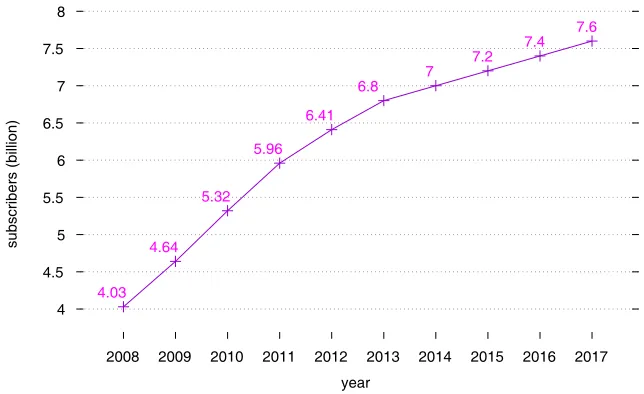
The exposure to radiofrequencies is still a topic under investigation, because of the increasing use of smart objects. The major exposure sources of people are these objects themselves (and especially mobile phones), and there exists no evidence yet of harm. Nevertheless, the mobile telephony base stations antennas can worry people living in the neighbourhood, and environmental associations are actively lobbying against the installation of new equipments. By the end of 2016, more than 7 billion mobile phone subscribers contract worldwide (see Figure 1) according to the ITU (International Telecommunication Union). As far as France is concerned there are 73 million mobile phone contracts subscribed to this day according to ARCEP (French Electronic Communications Regulation Authority). In this context, more and more people are demanding precautionary measures and a reduction of the existing exposure limits.
The subject of EMF (electromagnetic fields) exposure has been widely addressed in the literature during the past ten years. The only proven risk to this day is the increase of temperature of human tissues. As a consequence, standards and recommendations have been established by committees from all over the world, such as ANSI (American National Standards Institute) in North America or ICNIRP (International Commission on Non-Ionizing Radiation Protection) guidelines in European countries. These standards and guidelines have been frequently improved to take into account numerous aspects of exposure and to tackle emerging issues.
There are still debates concerning EMF exposure. These debates are fueled by the increasing penetration of radio technologies in the everyday life (mobile phones, wi-fi,. . .) and devices (electricity meters, . . .). Several stakeholders are concerned by the exposure question: state ministries, state
Received 24 September 2018, Accepted 12 November 2018, Scheduled 27 November 2018
* Corresponding author: Nicolas Noe ([email protected]).
1 CSTB, Lighting and Electromagnetism Division, Nantes, France. 2 CNRS, Universit´e de Poitiers, XLIM, UMR 7252, F-86000
4 4.5 5 5.5 6 6.5 7 7.5 8
2008 2009 2010 2011 2012 2013 2014 2015 2016 2017 4.03
4.64 5.32
5.96 6.41
6.8 7
7.2 7.4
7.6
subscribers (billion)
year
Figure 1. Worldwide mobile cellular subscribers (billion).
agencies, technical and research centers, mobile telephony operators and companies, environmental and users associations,. . .These actors may have divergent agendas, hence general agreement and objective views of the existing situation are hard to reach. As a consequence, there is still a need for widely accepted exposure indicators, and research has to be carried out for building knowledge of real exposure levels, taking into account current and future radio technologies.
The goal of this paper is to improve the evaluation of human exposure, focusing on the electric field variability, both in time and space. The paper is divided into five sections. Section 1 is this introduction. Section 2 is a state-of-the-art study of EMF exposure quantification. This section introduces the physical quantities of EMF exposure (SAR, electric field) and the exposure indicators found in the literature. This will allow us to identify exposure quantification issues. Section 3 is dedicated to the concept of exposure area. First propagation regions in a radio link are described, then these exposure areas are defined. They will be the basis of the exposure variability analysis in this paper. Section 4 details the methodology used in this study. It deals with the technical goals, the study data and the processing of results. Section 5 is dedicated to hourly profiles of instantaneous exposure over a day. Existing profiles are discussed, and a new profile is proposed. Section 6 addresses the question of averaging duration, in terms of radio technologies and exposure areas. Finally, Section 7 summarizes the contributions of this paper to the radiofrequencies (RF) exposure community.
2. ANALYSIS OF EXISTING APPROACHES AIMED AT QUANTIFYING THE EXPOSURE
We describe here the physical quantities used to quantify EMF exposure in existing norms and guidelines. These quantifies are as the follows:
• Electric field,
• SAR(Specific Absorption Rate, the power absorbed per mass of tissue)
Electric field can only be used to measure far field exposure levels, whereas SAR can be used both for near and far fields, and is to this day the only way to characterize near field exposure. These two quantities differ on the measurement and simulation processes. These quantities are used as thresholds for regulation enforcement, but there is a need to have dedicated tools to study real exposure.
project led to a general agreement of technical bases to use in current debates, and eased in France the comparison between heterogeneous exposure situations (domestic, industry, . . .). A main contribution concerning mobile telephony was the definition of a Global Exposure Indicator (GEI). This indicator aggregates SAR and electric field in a single value, depending on user’s behavior (duration of “voice” and ”data” usages). The major step forward with this indicator is that this single value handles the exposure from both downlink (base stations antennas) and uplink communications (phone). This GEI indicator was also used in a European project called LEXNET [3]. Its goal was to achieve efficient solutions to reduce RF human exposure by 50% without damaging the quality of service. This indicator enabled the analysis of the performance and relevance of low emission radio technologies.
All these studies illustrate the importance of the propagation region (near field, far field) on the exposure characterization. In this paper we will focus on the analysis of far field exposure to mobile telephony base stations. We will study the hypothesis that the variability of the electric field is characterized by the relative emitter/receiver location and visibility. This leads to the definition of exposure areas in the forthcoming section.
3. CONCEPT OF AREA OF EXPOSURE
3.1. Propagation Area
We recall in this section the importance of propagation regions in the radio transmission link. As a matter of fact, the properties of electromagnetic waves depend on the propagation region around the emitter. There are four propagation regions, depending on the distance to the emitter:
• Reactive near field
This is a very “thin” region, and it is located within a distance to the emitter shorter than 2λπ, with λbeing the wavelength. This is roughly 5 cm for a 900 MHz emitter. Waves are evanescent in this region, i.e., propagation phenomena are negligible compared to radiation phenomena. This region cannot be simulated accurately with wave propagation tools.
• Rayleigh region
This region ranges between 22λπ and D2λ2, with Dbeing the largest dimension of the antenna. For a one-meter-long 900 MHz GSM antenna, D2λ2 = 1.5 m). The electromagnetic power is confined within a cylinder around the radiating aperture. The wave might exhibit a cylindrical character as shown in [4].
• Fresnel region
This is an intermediary region between D2λ2 and 2Dλ2 from the emitter. The wave naturally diverges. On the upper limit of the Fresnel region, the aperture, as seen from the antenna, is equal to the angular aperture of the main lobe 2Dλ. The combination of Fresnel and Rayleigh region is thenear field regionof the antenna.
• Fraunhoffer region
This region is beyond a distance of 2Dλ2 and is also called far field region of the antenna. The radiated power is confined into a conic beam, and the waves are locally almost plane waves.
In an urban environment (exposure generated by base station antennas, on the ground or on facades of neighbouring buildings), we only deal with the far field region, for both measurements and simulations. Consequently, the far field region will be segmented into three exposure areas, defined in the following section.
3.2. The Concept of Exposure Areas
only have interest in far field. Thirdly, asymptotic methods are very fast in 2.5D urban environments [5– 7]. Finally, the contributions from each emitter to each receiver can be identified as direct, reflected and diffracted paths.
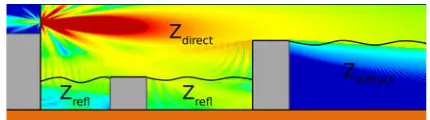
This identification of direct, reflected and diffracted paths leads to the definition of exposure areas using geometrical criteria only. For a given emitter, three exposure areas are identified:
• Zdirect is the area where most of the emitted power is collected, coming mainly from direct paths. The electric field in this area mostly depends on emitter characteristics. Reflected and diffracted paths might exist in this area, but their contributions are negligible with respect to the direct paths.
• Zreflection is the area where the collected power mostly comes from reflected paths. The electric field in this area mostly depends on the shape and the electromagnetic properties of the building surrounding the emitter. There is no direct path in this area.
• Zdiffractionis the area where the collected power only comes from diffracted paths. The electric field in this area mostly depends on the diffraction model and the height profile of the paths. A receiver is inZdiffraction when it is in neitherZdirect norZreflection areas.
Figure 2 illustrates these exposure areas.
Figure 2. Exposure areas (areas can be identified during ray-tracing computation).
As shown in [8], the variability of the electric field is correlated to the main contribution, so to the exposure areas. Thus we propose to study electric field variability in each of them. The next section describes the used methodology.
4. METHODOLOGY
4.1. Goals
Current standards and guidelines (ICNIRP, ANSI) require measurements to be continuously averaged over 6 minutes in order to evaluate short-term exposure. This duration only relies on health risk and has no other explanation than thermal hazard. Russia and Ukraine use an exposure threshold close to ICNIRP, but the threshold is a continuous function of the exposure duration [9] (concept of dose). In France, ANFR (National FRequency Agency) is responsible for EMF exposure protocols establishment. The French protocol, based upon ICNIRP standards, allows for a shorter measurement duration as long as the RMS (Root Mean Square) value is stable, but the stability criterion is not defined. A French study on public exposure to base stations showed that the exposure level, whatever the time of the day, is close to the one that would be measured and averaged over 6 minutes [10]. More recently, the LEXNET indicator [3] took into account the large-scale temporal variability of the exposure by segmenting day according to the human activities, leading to daytime and evening slots.
The goal of this study is to analyze temporal variability of public exposure to mobile telephony base station antennas. More specifically, we address the uncertainties on the temporal variability of the instantaneous exposure level, and so on the averaging duration to apply. Therefore, daily exposure for different mobile communication technologies is studied as the temporal variation of exposure in each different exposure area.
and over longer time periods is analysed. We have initiated our study with the same methodology and then have improved it with the exposure area concept, and its effects on temporal variability. In addition to existing technologies† at the time of [10], we also take into account LTE (Long Term Evolution) emitters that were not available at that time.
4.2. Fixed-Point Temporal Measurements
For EMF measurement we used the Narda SRM 3006 spectrum analyzer. This analyzer offers the possibility to selectively measure the EMF, per technology (GSM, UMTS, LTE. . .) and per frequency, to identify the exposure sources. It also computes the total field of all the transmitters radiating in the measurement environment. Thus two types of measures were performed:
• wide-band measurement (“safety” mode): record one value per downlink according to each frequency band allocated to operators. The “safety” mode is used to perform transient measurements;
• narrow-band measurement (“spectrum” mode): record of the detailed spectrum around a given central frequency.
In France the frequency spectrum is in the public domain. For telecommunication systems like mobile telephony, each mobile technology (GSM, UMTS, LTE) operates in a given frequency bandwidth (900 and 1800 MHz for GSM, 2100 MHz for UMTS and 2600, 800 and 700 MHz for LTE‡). These frequency bands are spread across four operators: Orange, SFR, Bouygues and Free. They are reserved for public mobile telephony, whereas other bands can be employed for professional, military or academic research communication purposes. In France the ARCEP is in charge of allocating the frequency spectrum to the different mobile operators, and the spectrum is presented on Figure 3 (data of 2014).
Figure 3. Frequency spectrum allocation to the different french operators (2014).
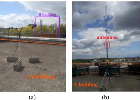
To analyze the temporal variability of the exposure, a measurement campaign was realized on the CSTB (Scientific and Technical Center for Building) site of Nantes. The measurement point is located on the ceiling of the A building, as it is illustrated on Figure 4. The base stations of Orange and SFR are also in the site. The Orange base station is installed on the B building (cf. Figures 4 and 5(a)), the
Figure 4. Measurement site of CSTB: measurement site (building A) and base stations of Orange (building B) and SFR (mast).
Main radiating azimuth
(b) (a)
Figure 5. Base stations: (a) Orange, (b) SFR.
measurement point being in its main radiating azimuth (cf. Figure 5(a)), whereas the SFR base station is on a mast (cf. Figure 5(b)). Figures 6(a) and 6(b) show the two base stations from the point of view of the measurement point. The measurement point has been chosen to receive EMF in Zdirect (in the main azimuth) from the Orange transmitter which is in line of sight and EMF in Zdirect and Zreflection from the SFR transmitters.
(b) (a)
Figure 6. Base stations from the point of view of the measurement point: (a) Orange, (b) SFR.
Zdiffraction, numerous external factors (moving vehicles. . .) can influence the measurement. The analyzer has been configured to measure the cumulative electrical field in each downlink bandwidth affected to each operator (safety mode). Even if some frequency bands can be used by several technologies (for instance GSM and UMTS in the 900 MHz band, or GSM and LTE in the 1800 MHz for Bouygues), the knowledge of the transmitters located in the area of interest (public data from ANFR) combined with the analysis of the measured spectrum allows to identify the measured technology, which are:
• InZdirect (Orange, located in the area of interest): LTE 800, GSM 900 and 1800, UMTS 2100,
• InZreflection (SFR, located in the area of interest): LTE 800, UMTS 2100§,
• InZdiffraction (Bouygues Telecom, not located in the area of interest, they are at about 400 m from the measurement point): LTE 800, GSM 1800, UMTS 2100.
Two types of measurements have been performed to analyze the temporal variability of the exposure:
• Measurements during 6 hours (Meas 6h): Measurements by downlink bandwidth during the day with a temporal step of 6 s, on a total duration of 6 h.
• Measurement during 24 hours (Meas 24h): Measurements per downlink bandwidth with a temporal step of 12 s at the same receiving location as for Meas 6h, on a total duration of 24 h.
To characterize the temporal variability of the exposure to EMF, we were interested in the influence of the exposure areas on the averaging duration according to each technology (GSM, UMTS and LTE), from the two previous types of measurements. We also searched to quantify the averaging duration required to obtain a better characterization of the exposure.
5. SEGMENTATION INTO DAILY EXPOSURE PROFILES
This segmentation is performed with the 24 hour-long measurements (Meas 24h).
5.1. Previous Work
Mobile telephony usage is linked to human activity, and it highly depends on the time of the day, with strong differences between day and night. As a consequence it is assumed that daily exposure can be divided into two different variation profiles. The study presented in [11] compares global average exposure to 3G (both downlink and uplink) in urban, suburban and rural areas. This leads to these two profiles:
• Day-profile: 8AM-6PM • Evening-profile: 6PM-8AM
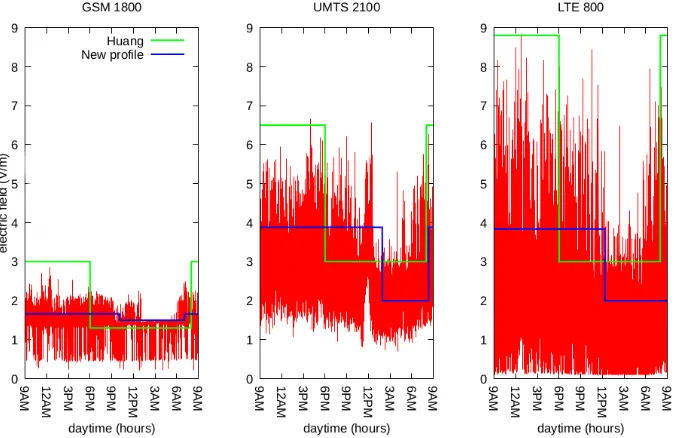
Nevertheless when other technologies are taken into account and focusing on downlink only, we identify different segmentation profiles. This is illustrated with measurements in Zdirect exposure area in Figure 7. This figure displays instantaneous exposure during 24 hours for GSM, UMTS and LTE. The measurement time is on the horizontal axis (in hours, starting at 10 AM, until the next morning), and the electric field level (in V/M) in the considered downlink band is on the vertical axis. Segmentation profile proposed in [11] is also plotted in green (high part: day-profile, low part: evening-profile).
Figure 7. Time dependant exposure to an Orange base station during 24 hours.
Figure 7 obviously displays two temporal profiles: a lower exposure profile (mostly during nighttime) and a higher exposure profile (mostly during daytime). This corroborates the basic hypothesis that the exposure to base stations is directly linked to daily human activity, with higher values at daytime and lower values at nighttime.
Nevertheless even if the limit between these two profiles is hard to identify, it is also blatant that segmentation proposed in [11] does not apply to this signal. As a consequence, a segregation technique is used to compute the limit with objective criteria.
5.2. New Profiles
A new segmentation procedure is now introduced. It consists in defining two adjacent time periods, each with its own average value. We then have to look for the “breaking point” between these two parts. This breaking point should satisfy that the difference between the average levels should be as great as possible, whereas the duration of each part should be as long as possible. We can then define theEopt parameter to maximize in order to fit both criteria as:
Eopt =|E2−E1| ∗
T1∗T2 (1)
T1 and T2 are the respective durations of the two profiles (hence T1+T2 = 24 h), and E1 and E2
are the average electric field values on the two profiles.
relative errorEr betweenE1 andE2 is defined in Equation (2) while the differenceEc betweenE1 and
E2 is defined in Equation (3).
Er = E1E−E2
2
(2)
Ec = 20 log E
1
E2
(3)
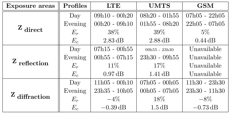
Table 1 shows segmentation results for the three exposure areas and the three considered technologies (GSM, UMTS, LTE): time slot for each of the two profiles, relative error Er (in%) and differenceEc (in dB).
Table 1. Comparative daily profiles according to exposure areas and technologies.
Exposure areas Profiles LTE UMTS GSM
Z direct
Day 09h10 - 00h20 08h20 - 01h55 07h05 - 22h05 Evening 00h20 - 09h10 01h55 - 08h20 22h05 - 07h05
Er 38% 39% 5%
Ec 2.83 dB 2.88 dB 0.44 dB
Z reflection
Day 07h15 - 00h55 09h55 - 23h30 Unavailable Evening 00h55 - 07h15 23h30 - 09h55 Unavailable
Er 11% 17% Unavailable
Ec 0.97 dB 1.41 dB Unavailable
Z diffraction
Day 11h05 - 00h10 07h05 - 00h05 11h30 - 23h30 Evening 23h35 - 10h05 00h05 - 07h05 23h30 - 11h30
Er −4% 18% −8%
Ec −0.39 dB 1.5 dB −0.73 dB
Zdirect: The analysis ofEc andEr(see Table 1) shows that LTE and UMTS technologies have larger gap than GSM in the two profiles inZdirectarea. In other words, the exposure to these two technologies is very different in the daytime compared with the night.
Zreflection and Zdiffraction: The difference between the two profiles is lower than 2 dB in theZreflection and Zdiffraction exposure areas, whatever the technology. It can also be noted that the relative error Er is negative for LTE and GSM inZdiffraction area, meaning that the average night-profile signal is slightly higher than the average day-profile one. Furthermore, theEr values for LTE (−4%) and GSM (−8%) in these areas, compared to the values in visibility area (except for GSM) show that the average variations of the two profiles are identical.
In conclusion it is mostly theZdirectarea that is influenced by the day and night change for LTE and UMTS technologies (38% for LTE, 39% for UMTS). We will now see if these conclusions are confirmed by studying the variation rate of the EMF as a function of the averaging duration, for each profile (day or night), in order to quantify the minimum duration needed to assess exposure accurately.
6. QUANTIFICATION OF AVERAGING DURATION
6.1. Data Processing of Measurements
Let E[t] be the instantaneous measurement (sampled every 6 seconds) of the electric field for a full duration of 6 hours. ΔT is the duration (in seconds) of the time averaging window, and NΔT is the
number of samples in the current time averaging window. The smoothed counterpart of signal E[t] is ¯
to remove transient fluctuations of the signal and to highlight long term tendencies. ¯E[t,ΔT] is defined as:
¯
E[t,ΔT] = 1 NΔT
NΔT−1
k=0
E[t−k] (4)
6.2. Influence of Exposure Areas and Technologies
This study is based on 6 hour-long measurements (Meas 6h cf. Subsection 4.2).
6.2.1. Study of Signal E¯[t,ΔT]
Figure 8 shows that for Orange LTE 800 in Zdirect area, the measured signal during 6 hours as a function of time, smoothed for each of these five ΔT values: ΔT1 = 60 s, ΔT2 = 360 s, ΔT3 = 720 s,
ΔT4 = 1800 s, ΔT5 = 3600 s. Time (in minutes) and electric field (in V/M) are displayed on thex and
y-axes, respectively. The raw signal (sampled every 6 s) has unpredictable short time variations. As a consequence, time averaging is mandatory to make a reliable analysis of exposure. By using a sliding averaging window (of different durations), the signal becomes more and more stable. This is true for all technologies and all exposure areas. We now study the effect of ΔT according to technologies and exposure areas.
0.5 1 1.5 2 2.5 3 3.5 4 4.5 5 5.5 6
0 50 100 150 200 250 300 350 400
electric field (V/m)
time (minutes)
ΔT1
ΔT2
ΔT3
ΔT4
ΔT5
Figure 8. Effect of averaging duration on the electric field level — Orange LTE 800 — ΔT1 = 60 s,
ΔT2 = 360 s, ΔT3 = 720 s, ΔT4= 1800 s, ΔT5 = 3600 s−Zdirect.
6.2.2. Influence of ΔT According to Technologies and Exposure Areas
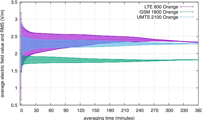
Here the influence of technology and exposure area on the evolution of ¯E[t,ΔT] is emphasized. It will be done using an “error bars” graphical representation. This representation is well suited to study data variability, showing both average value as the center value and RMS value as an interval around it. It would highlight the potential significant differences in the variability of the electric field depending on the technology. These graphs show the evolution of ESΔT as a function of ΔT (see Equation (5)).
ESΔT is an interval depending on μΔT (average value of ¯E[t,ΔT], see Equation (6)) and σΔT (RMS
value of ¯E[t,ΔT]). If the values are distributed with a normal (Gaussian) law, 68% of these values are in the range ESΔT defined with:
0.5 1 1.5 2 2.5 3 3.5
0 30 60 90 120 150 180 210 240 270 300 330 360
average electric field value and RMS (V/m)
averaging time (minutes)
LTE 800 Orange GSM 1800 Orange UMTS 2100 Orange
Figure 9. ESΔT according to technologies for Orange inZdirect.
0.05 0.1 0.15 0.2 0.25 0.3
0 30 60 90 120 150 180 210 240 270 300 330 360
average electric field value and RMS (V/m)
averaging time (minutes)
LTE 800 SFR UMTS 2100 SFR
Figure 10. ESΔT according to technologies for SFR inZreflection.
μΔT =
1 T
T
t=0
¯
E[t,ΔT] (6)
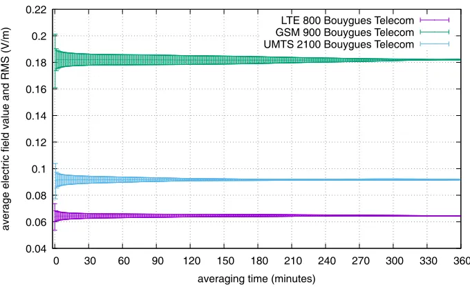
Figure 9 represents the evolution of ESΔT according to technologies for Orange in Zdirect, while Figures 10 and 11 show the ones for SFR in Zreflection and Bouygues in Zdiffraction, respectively. Each exposure area is hence treated.
The comparison of curves of Figures 9, 10 and 11 shows that the variations ofESΔT are far greater
in the Zdirect area where σΔT goes up to 1.5 V/M, compared to Zreflection and Zdiffraction, whereσΔT is
0.04 0.06 0.08 0.1 0.12 0.14 0.16 0.18 0.2 0.22
0 30 60 90 120 150 180 210 240 270 300 330 360
average electric field value and RMS (V/m)
averaging time (minutes)
LTE 800 Bouygues Telecom GSM 900 Bouygues Telecom UMTS 2100 Bouygues Telecom
Figure 11. ESΔT according to technologies for Bouygues inZdiffraction.
the radio technology from a circuit-oriented connection to a packed-oriented connection, hence allowing multiple users to communicate at the same time [13]. As far as LTE is concerned, its radio interface is based on multiplexing and OFDMA, allowing high flow communication with fewer interferences and a full-IP network architecture [14], which implies very fast signal variations.
The results globally show that the exposure area has a great impact on exposure evaluation. Temporal evaluation of the exposure also depends on the technology in Zdirect area. Beside, exposure evaluation is less affected by technologies in the Zreflection and Zdiffraction areas, because of the influence of the environment. We will now focus on the averaging duration to apply, for each exposure area and each technology.
6.3. Determination of averaging duration
In this part we study the averaging duration needed to be able to quantify exposure levels. A first study led to the segmentation of exposure in variation profiles, depending on the time of the day. Then the averaging duration needed to have exposure varying less than a given variation rate is analyzed. Hence, the variation rate T VΔT given by Equation (7) is computed.
T VΔT = σΔT
μΔT
(7)
In order to assess the averaging duration for each variation profile, a criterion of signal stability is defined based on conclusions of COPIC (French’s comity on mobile telephony exposure) [10]. This project concluded that, as far as mobile telephony is concerned and for current technologies (GSM and UMTS at the time of the study) and current usages, the measured exposure level during the day, whatever the time of the day, was close to the one that would be measured and averaged over 6 minutes. Furthermore, the amplitude of the variations during the day was rather low, less than 30%. As a consequence, we set our variation rate to 30%.
Table 2 displays the averaging duration ΔT found for each profile so as to reach a T VΔT (cf.
Equation (7)) lower than 30%. The average signal valueμΔT (cf.Equation (6)), averaged with ΔT, was
also indicated for each profile in order to compare average differences between profiles, as a function of the variation rate.
Table 2. ΔT and μΔT for a variation rate lower than 30% according to each exposure area and
technology.
Areas Profiles LTE UMTS GSM
Z direct
ΔT μΔT (V/m) ΔT μΔT (V/m) ΔT μΔT (V/m)
Day 1 min 2.52 1 min 2.91 12 s 1.48
Evening 1 min 1.88 1 min 2.13 12 s 1.41
Z reflection EveningDay 12 s12 s 0.120.10 12 s12 s 0.240.20 UnavailableUnavailable UnavailableUnavailable
Z diffraction EveningDay 12 s12 s 0.130.14 12 s12 s 0.130.11 12 s12 s 0.170.18
Table 3. ΔT and μΔT for a variation rate lower than 10% according to each exposure area and
technology.
Areas Profiles LTE UMTS GSM
Z direct
ΔT μΔT (V/m) ΔT μΔT (V/m) ΔT μΔT (V/m)
Day 24 min 2.64 54 s 2.93 1 min 1.52
Evening 20 min 1.92 8 min 2.14 1 min 1.42
Z reflection EveningDay 1 min12 s 0.120.10 2 min1 min 0.230.20 UnavailableUnavailable UnavailableUnavailable
Z diffraction EveningDay 12 s12 s 0.130.14 1 min1 min 0.120.11 1 min1 min 0.170.18
analysis of the previous section and agree with COPIC conclusions [10]: in order to evaluate daily exposure at a given location, it is not needed to take into account the whole time slot. An averaged measurement of a few minutes is sufficient enough. Daily exposure can be evaluated with a 1 min measurement as long as the location is inZreflection orZdiffractionarea, whatever the technology (even for LTE) and the moment of the day. On the opposite, as far as Zdirect is concerned, day and night profiles should be taken into account since a difference of μΔT equal to 0.8 V/M is observed between day and
night for LTE and UMTS. However if the variation rate is changed, these conclusions can change a lot as illustrated in Table 3, where the same study has been conducted with a variation rate lowered to 10%.
This example shows that the exposure area highly influences the averaging duration to be used for exposure quantification for LTE and UMTS.
When the location of the measurement point is in non-line of sight with the emitter (Zreflection and Zdiffraction), the averaging duration can be reduced to 2 min. For example, Figure 12 presents a zoom on the first part of Figure 11 (Zdiffraction) corresponding to averaging durations between 0 and 12 min. The result concerning UMTS 2100 (Bouygues Telecom) shows that an averaging duration of 6 min (recommended by ANFR) gives a variation rate T VΔT of 4%, which is in accordance with the
objective of 10%. But it can also be observed that an averaging duration of 2 min is sufficient since it gives a T VΔT of 5.5%.
On the opposite, in line of sight of the emitter (Zdirect), the averaging duration can be larger than the protocol one (20 min to 24 min depending on the profile for LTE and 8 min to 9 min for UMTS). Figure 13 illustrates this point for Orange in Zdirect. In this case, whereas an averaging duration of 24 min almost respects the target variation rate of 10% (we have 13%), using the averaging duration of 6 min recommended by the protocol drives to a variation rate of 42%, that is almost 4 times more. This difference between exposure areas is related to the effects of the environment. This implies that the variation rate T VΔT is a very important parameter to quantify exposure, especially for LTE and
Figure 12. ESΔT according to technologies for Bouygues inZdiffraction (zoom of Figure 11).
Figure 13. ESΔT according to technologies for Orange inZdirect (zoom of Figure 9).
7. CONCLUSION
The influence of the evaluated point location has been studied with regard to the transmitters by taking into account the daily profile. The conclusion is that inZdirect, the daily profile has to be taken into account to better characterize the exposure.
The conclusions of this paper are:
• the exposure areas can be divided in two specific ones: Zdirect and Zindirect (Zreflection,Zdiffraction); • the daily profile (day/night) has to be taken into account for the mean level evaluation intoZdirect
(LTE and UMTS);
• the duration of averaging (6 min) should be decreased to 1 min according to a variation rate of 30%. Thus, we have verified the proposed hypothesis by showing that the exposure area influences the assessment of the real exposure, and that it has to be taken into account to better characterize the exposure. From a practical point of view, this study can be a base to achieve optimized guidelines to measure electric field exposure from mobile telephony base stations. First, the two proposed exposure areas can be easily identified on a simple geometrical criterion (line of sight of the emitter or not). Then, public data from ANFR are used to know what technology from what operator is deployed in the considered environment. Finally, Tables 1 and 2 give the good averaging duration to use according to a specific technology and the moment of the day.
This study presents some solutions to measure the exposure. Nevertheless, some aspects can be improved due to the complexity of the problem. However, we are confident to conclude that an indicator depending on the exposure area, the exposure duration and the technology should better quantify the far field exposure in a given location. For the exposure at urban scale, it would be interesting to integrate new parameters as the population density, the spatial averaging and the exposure area to provide exposure maps that would be sufficient representative of the real exposure. For indicators as in [2, 3, 15], which also integrate the near field, the consideration of exposure areas should improve the estimation of the exposure level by adapting the index according to each one.
REFERENCES
1. Ghanmi, A., “Analyse de l’exposition aux ondes ´electromagn´etiques des enfants dans le cadre des nouveaux usages et nouveaux r´eseaux,” Ph.D. Thesis, Universite Paris-est Marne-La-Vallee, 2015. 2. Gaudaire, F., J. Caudeville, P. Demaret, J. Wiart, and C. Person, “D´efinition d’indicateurs pour la caract´erisation de l’exposition radio´electrique,” https://www.anses.fr/fr/system/files/RSC121015-DossierParticipant.pdf, 2015.
3. Wiart, J., “Low EMF exposure networks,” http://www.lexnet.fr/, 2015.
4. Cicchetti, R., A. Faraone, and Q. Balzano, “A uniform asymptotic evaluation of the field radiated from collinear array antennas,”IEEE Transactions on Antennas and Propagation, Vol. 51, No. 1, 89–102, 2003.
5. No´e, N., F. Gaudaire, and M. D. B. L. Ndiaye, “Estimating and reducing uncertainties in ray-tracing techniques for electromagnetic field exposure in urban areas,”2013 IEEE-APS Topical Conference on Antennas and Propagation in Wireless Communications (APWC), 652–655, Sept. 2013. 6. Combeau, P., L. Aveneau, R. Vauzelle, and Y. Pousset, “Efficient 2-D ray-tracing method for
narrow and wideband channel characterisation in microcellular configurations,” IEE Proccedings on Microwave Antennas and Propagation, Vol. 153, No. 6, 502–509, Dec. 2006.
7. Alwajeeh, T., P. Combeau, R. Vauzelle, and A. Bounceur, “A high-speed 2.5D ray-tracing propagation model for microcellular systems, application: Smart cities,” IEEE EUropean Conference on Antennas and Propagation (EUCAP), Paris, France, Jan. 2017.
8. Ndiaye, M. D. B. L., N. No´e, P. Combeau, Y. Pousset, and F. Gaudaire, “Analysis of electric field spatial variability in simulations of electromagnetic waves exposure to mobile telephony base stations,” European Conference on Antennas and Propagation (EUCAP), Lisbon, Portugal, Apr. 12–17, 2015.
10. COPIC, “Diminution de l’exposition aux ondes ´electromagn´etiques ´emises par les antennes relais de t´el´ephonie mobile,”Technical Report, Le minist`ere de la sant´e, avec le concours du minist`ere du d´eveloppement durable et du secr´etariat d’´etat charg´e de la prospective et du d´eveloppement de l’´economie num´erique, 2013.
11. Huang, Y., A. Krayni, A. Hadjem, J. Wiart, C. Person, and N. Varsier, “Comparison of the average global exposure of a population induced by a macro 3G network in urban, suburban and rural areas,”Radio Science Conference (URSI AT-RASC), 2015 1st URSI Atlantic, 1-1, May 2015. 12. 3GPP, “Ts 45.002: 3rd generation partnership project; technical specification group radio access network; GSM/edge multiplexing and multiple access on the radio path (release 4),” Technical Report, 3GPP, 2000.
13. 3GPP, “Ts 25.101/102: 3rd generation partnership project; technical specification group radio access network; User equipment radio transmission and reception (release 4),” Technical Report, 3GPP, 2001.
14. 3GPP, “Ts 36.212: 3rd generation partnership project; evolved universal terrestrial radio access (E-UTRA); Multiplexing and channel coding (release 8),” Technical Report, 3GPP, 2006.