Correlation Analysis of Two Skewed Dipoles Using Embedded
Beam Patterns
Jung-Hoon Han1, * and Noh-Hoon Myung2
Abstract—In this paper, the correlation coefficients of skewed dipole arrays for antenna diversity are theoretically analyzed for each polarization characteristic and in various propagation environments. The correlation is not simply increased by two closely located antennas with different polarization characteristics, nor is it decreased by increasing the distance between the antennas. This is interpreted from the correlation analysis of two skewed dipoles with different polarization characteristics. The embedded beam patterns of the two skewed dipoles are calculated using the mutual impedances derived using the effective length vector (ELV) method; then, the mutually coupled correlation coefficients forθ, φ, and total polarizations are effectively derived. The correlations are also analyzed for various realistic propagation environments using statistical channel models with angular density functions, and cross polarization discriminations (XPDs). Finally, this paper provides an effective correlation analysis for two dipoles and proposes an optimal geometry for two skewed dipoles in various propagation environments for each polarization characteristic with environmental variables.
1. INTRODUCTION
The performance degradation of mobile and wireless systems in multipath propagation environments, called the signal fading phenomenon, can be managed successfully with spatial, polarization, pattern, and another diversity schemes [1–3]. In communication systems, most theories use point source analyses for isotropic radiation or simple linear antenna arrays for co-polarization transmitting and receiving, and even use two-dimensional models for analysis [4, 5]. However, three-dimensional models need to be considered for realistic multiple scattering environments and environmental factors must also be considered including the vertical and horizontal polarization propagation characteristics with cross polarization discriminations (XPDs) for realistic multipath channels.
Dipoles and monopoles are often used to analyze the antenna diversity of linear antennas. The polarization diversity has been developed using orthogonal and tilted linear antennas through vertically polarized mobiles with XPDs of the incident fields [2]. Experiments using spatial, polarization, and pattern diversities have been also conducted using dipole [3]. Many studies on monopole applied antennas combining broadband and the meta-material characteristics have been carried out [6, 7]. Moreover, Tri-pol antenna consists of three standard sleeve monopoles orthogonally arranged [8]. Together, these three antennas can create an arbitrary vector electric dipole moment at the transmitter and receiver. Vertically polarized dipoles or monopoles on the ground have been demonstrated with mutual coupling (MC) effects with variations in the spatial separation between antennas for antenna diversity [9, 10]. Furthermore, true polarization diversity (TPD) has been proposed in order to achieve a high diversity gain using an inclined dipole array to receive various polarized waves for multipath fading channels [11–13]. Finally, dipoles have been applied to antenna diversity systems, and they have been
Received 26 April 2018, Accepted 9 August 2018, Scheduled 16 August 2018 * Corresponding author: Jung-Hoon Han (junghoon [email protected]).
interpreted in several research articles. One of the reasons of frequent use is that the three-dimensional power gain patterns of dipole are expressed using numerical formulas according to the dipole geometries for each polarization [14].
The correlation coefficient is the key factor for evaluating the antenna diversity performance that is calculated using the antenna field patterns [1]. There are many researches about the correlation analysis of the antenna diversity. Switched parasitic elements have enabled useful implementations of antenna pattern diversity and evaluations using pattern correlations [15]. The correlation analysis of simple point sources was achieved using closely spaced linear, vertically polarized antennas [16]. Furthermore, the spatial correlation coefficients of signals received by two normal mode helical antennas in a multipath environment have been characterized using mutual impedance estimations [17]. The correlation coefficients between received signals by two antennas have been calculated usingS-parameters at ports with antenna radiation efficiencies [18]. Moreover, the spatial correlation estimation using two closely coupled electrical dipoles has been discussed as a function of the load impedances for low correlation [19]. An analytic expression for the spatial correlation of uniform rectangular half-wavelength dipole arrays has been derived considering the elevation and azimuth spread power spectrum [20]. Furthermore, an approximate spatial correlation formulation of arbitrary angle of arrival scenarios has been presented for three-dimensional spatial correlations with the antenna mutual coupling [21].
The antenna correlation is closely associated with the antenna mutual coupling. Thus, the mutual impedance calculations of two dipoles are the most important processes for solving the correlations. Several studies have been conducted on the mutual impedance between parallel dipoles in echelon configurations. King [22] proposed exact expressions that were developed for the mutual impedance between two staggered parallel linear antennas; other advanced analysis techniques have been introduced from these derivations [23–25]. For the coplanar-skew configurations, several studies have been presented [26–29]: Representatively, Richmond [27] introduced the induced electromotive force (EMF) formulation of mutual impedance between coplanar-skew dipoles. Furthermore, nonplanar-skew cases have also been investigated [30–33]; for example, Richmond [30] introduced an expression for the mutual impedance of nonplanar-skew dipoles. However, this approach is complicated because the integral path for calculating the mutual impedance lies along the radial directions from the origin point, i.e., the intersection point of two coplanar-skew dipoles. Thus, the integration requires a different axis, which is in the radial direction via the radiated fields from the transmitting dipole, and transformations of variables. For nonplanar-skew cases, the geometrical structure is complicated, and the proposed formula requires transformations of the variables as well. This paper utilizes an effective estimation method for the mutual impedance between two nonplanar-skew dipoles: the effective length vector (ELV) method is used for precise, simple, and intuitive analyses [29, 34].
environments and each polarization with variations in the dipole geometries. Section 4 concludes the paper.
2. EMBEDDED BEAM PATTERNS USING MUTUAL IMPEDANCE
Calculation of the correlation coefficients for two antennas is an important issue when evaluating the performance of an antenna diversity system. The correlation analysis of two dipoles must consider the mutually coupled beam patterns using the adjoining dipole; this is called an embedded beam pattern [36, 37]. Furthermore, correlation is closely associated with mutual coupling between dipoles. Thus, when two skewed dipole arrays are considered, it is essential to calculate the mutual impedance between two arbitrarily skewed dipoles. In this section, a method of calculating the mutual impedances is discussed and the embedded beam patterns are derived using the mutual impedances.
2.1. Mutual Impedance of Skewed Dipoles
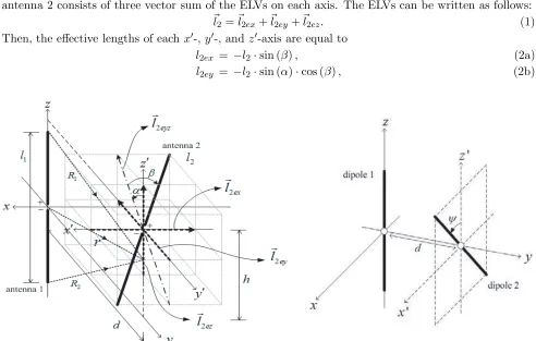
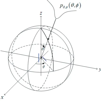
Exact calculation of the mutual impedance is important for the embedded beam pattern calculation. There are several methods to calculate the mutual impedance between two arbitrarily positioned and skewed dipoles. Among them, the easiest and most accurate method is adopted [29, 34]: this method uses the ELVs of the skewed dipoles with a modified induced electromotive force (EMF) method. The ELVs are obtained from the projections on the newly defined coordinate axes ofx,y, and z as indicated in Fig. 1. The mutual impedance is calculated by multiplying the radiated electric field from the antenna 1 by the current distribution on the antenna 2 using the induced EMF method. The radiated electric field from the transmitting dipole, which is the antenna 1, lies on thez-axis of the Cartesian coordinate system, but only exist along the z- and y-axes. The antenna 2 is slanted by an angle α on the same plane as the antenna 1 and an angle β between the ELVs for the yz-plane and the antenna 2. The antenna 2 consists of three vector sum of the ELVs on each axis. The ELVs can be written as follows:
l2 =l2ex+l2ey+l2ez. (1)
Then, the effective lengths of each x-, y-, and z-axis are equal to
l2ex = −l2·sin (β), (2a)
l2ey = −l2·sin (α)·cos (β), (2b)
Figure 1. Geometry of two arbitrarily positioned and skewed dipoles.
l2ez = l2·cos (α)·cos (β), (2c) where l2 is the length of the antenna 2, and α is the slant angle of the antenna 2 on the yz-plane. The nonplanar slant angle is defined as β, which is an angle between the effective length vector of the yz-plane and antenna 2. Thus, the mutual impedance can be calculated using integrations along these effective lengths and their sum. Then, the mutual impedance is expressed as
Z21 = Z21z+Z21y
= −30
sin kl1 2 sin kl2ez 2
h+l22ez
h−l22ez sin
k
l2ez
2 − |z−h|
−je−jkR1z(z) R1z(z)
+−je
−jkR2z(z)
R2z(z)
+j2 cos
kl1 2
e−jkrz(z) rz(z)
dz
+ −30
sin kl1 2 sin kl2ey 2 d+ l2ey
2
d−l22ey sin
k
l2ey
2 − |y−d|
h−l1
2
je−jk1y(y) R1y(y)
+
h+ l1 2
je−jkR2y(y) R2y(y) −j
2hcos
kl1 2
e−jkry
ry(y)
dy
y (3)
forh= 0 in Fig. 1.
The result is composed of the z- and y-axes components related to the effective length vectors. However, the x-axis does not need to be considered because the integral along the effective length of the x-axis is canceled through symmetry. When the angle β changes to a fixed angle α, the effective length for the integration is reduced or increased according to the change in angle, and the integral path also changes. The choice of integral path is important. The dipole has two poles, positive and negative. The induced potentials generated at the dipole terminals are calculated through the integration of the negative end to the positive end of the dipole. Therefore, this integral path direction can be defined as a vector concept.
The other parameters are defined as follows:
rz(z) = d2+z2, ry(y) = h2+y2,
R1z(z) =
d2+ (z−l1/2)2, R1 y(y) =
(h−l1/2)2+y2,
R2z(z) =
d2+ (z+l1/2)2, R2 y(y) =
(h+l1/2)2+y2,
(4)
wherel1 is the length of the antenna 1,dthe distance, andh the height between the centers of the two antennas as indicated in Fig. 1.
2.2. Embedded Beam Patterns of Skewed Dipoles
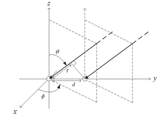
The geometry of the two skewed dipoles used to analyze the correlation coefficient of the mutually coupled beam patterns for each polarization is presented in Fig. 2. The dipole 2 is slanted with an angle (ψ) on the xz-plane with a distance (d) for each center point of the dipoles. First, the unmodified beam patterns of a dipole for each polarization must be considered. The geometry of the half-wavelength dipole and a relative spherical coordinate system are shown in Fig. 3. The dipole is on the xz-plane inclined at an angle (ψ) from the z-axis. The current distribution on the dipole is assumed to be sinusoidal, as follows:
I =I0cos (kl), (5)
for −λ/4 ≤l ≤ λ/4 and k = 2π/λ, where k is the wavenumber, andλ is the wavelength. Then, the dipole gain patterns for each polarization are as follows [14]:
Gθ = 1.641 (cosθcosϕsinψ−sinθcosψ)2
cos2(πξ/2)
Figure 3. Geometry of the half-wavelength dipole and relative coordinate system.
Figure 4. Geometry used to calculate the phase difference of the receiving wave for two receive points.
Gϕ = 1.641 sin2ϕsin2ψ
cos2(πξ/2)
(1−ξ2)2 , (6b)
whereξ = sinθcosφsinψ+ cosθcosψ.
The total gain can be expressed as the sum of the two gains of each polarization. As used for the directivity, the partial gain of the antenna can be defined for a given polarization in a given direction. The parts of the radiation intensity corresponding to the given polarization are divided by the total radiation intensity that would be obtained if the power accepted by the antenna was isotropically radiated. Then, with this definition for the partial gain, in a given direction, the total gain is the sum of the partial gains for any two orthogonal polarizations. For a spherical coordinate system, the total maximum gain (G) for the orthogonalθandφcomponents of the antenna can be written as follows [38]:
Gtot(θ, ϕ) =Gθ(θ, ϕ) +Gϕ(θ, ϕ). (7)
There are several methods of calculating the mutually coupled beam patterns [36, 39]. Kildal [36] proposed a method using the mutually excited current matrix obtained from the mutual, self, and load impedances. Then, the mutually coupled beam patterns, including the effects of the surrounding elements, which are called the embedded beam patterns, can be easily calculated. The radiation efficiency of the antenna system is excluded. Since the dipoles are located close to each other, they affect the radiation pattern of each other. The embedded beam patterns of the coupled dipoles (1 and 2) when the dipole 1 or 2 is excited are calculated as follows:
Gemb1 (θ, ϕ) = G1(θ, ϕ) +C1·G2(θ, ϕ)ejkτ, (8a) Gemb2 (θ, ϕ) = C2·G1(θ, ϕ)e−jkτ+G2(θ, ϕ), (8b) where G is the antenna gain pattern of the antenna 1 or 2. k is the wavenumber, and τ is the phase difference of the two incoming waves when the two antennas are on they-axis with a distance of d as shown in Fig. 4. Then,τ can be expressed as follows:
τ =dsin (ϕ) sin (θ). (9)
Furthermore, the parameter C is a coupling coefficient:
C1 =− Z21
Zi+ZL, C2
=− Z12 Zi+ZL.
(10)
values, but the mutual impedance (Z21) is a variable value according to the antenna distance or other geometrical parameters. Self-impedance can be calculated using the induced EMF method, which is valid for a thin wire dipole. For the sinusoidal current distribution, when a dipole is lying on thez-axis, the input impedance can be expressed as follows:
Zi = −
30 sin2(kl/2)
l 2
−2lsin
k
l 2 −z
−je−jkR1
R1 +
−je−jkR2
R2 +j2 cos
kl 2
e−jkr
r
dz, (11)
whereρ is the radius of the dipole,l the length of the dipole, and
r = ρ2+z2, (12a)
R1 =
ρ2+ (z−l/2)2, (12b)
R2 =
ρ2+ (z+l/2)2. (12c)
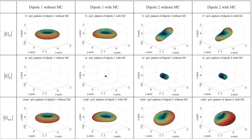
The load impedance (ZL) is assumed to be 50 Ω for impedance matching. According to the formulas, the absolute gain patterns of a single dipole without mutual coupling (MC) and embedded dipoles for the geometry in Fig. 2 are indicated in Fig. 5 according to each polarization when the antenna geometry hasd= 0.3λandψ= 45◦. The dipole gain pattern with MC is modified by other dipole located closely. The gain pattern of theθcomponent is unexpectedly modified and the gain pattern of theφcomponent is the same shapes, but the magnitude is formed or changed by the MC. Therefore, the correlations must be analyzed according to each polarization because the aspects of the transition differ depending on the polarization and the effects on the correlation also differ from each polarization. Consequently, the final correlation must be analyzed according to the aspects of each polarization.
Dipole 1 without MC Dipole 1 with MC Dipole 2 without MC Dipole 2 with MC
Gθ
Gφ
tot
G
3. CORRELATION ANALYSIS FOR VARIOUS ENVIRONMENTS AND EACH POLARIZATION
Antenna diversity is a well-known technique for reducing the effects of the fading phenomenon. When there are more than two antennas for the antenna diversity, their locations and geometrical structures are important. In practice, current portable devices must be small due to usability and device size limitations. Thus, the antenna radiation patterns are affected by nearby elements. Antenna MC is a key factor in the radiation beam pattern modifications and is called embedded beam pattern. The correlation analysis between the embedded beam patterns of each antenna element is a significant analysis indicator for an antenna diversity system. The antenna radiation pattern consists of θ and φ polarization components. The calculations of eachθand φpolarization correlation using the embedded beam patterns are performed in this section and they have different characteristics with skewed dipoles in rich scattering channels. Furthermore, the environment variables, which are the angular density functions of the incoming waves and cross-polarization discriminations (XPD) for fading channels, are also included for various multipath propagation environments.
3.1. Uniform and Isotropic Multipath Propagation Environments
After considering the MCs of two skewed dipoles, the embedded beam patterns are provided in Section 2.1. In a uniform and isotropic multipath propagation environment, which is common in rich scatterings, according to eachθ andφpolarization component, the mean value of the field is zero. The correlation coefficient is related to the radiated fields of each antenna and is also concerned with the receiving voltages. Each received voltage at the antenna 1 and 2 is proportional to the embedded beam patterns of each antenna. Thus, the envelope correlation coefficient between the two closely located antennas can be expressed as follows [1, 36]:
ρθ(φ,tot)=
4π
G1emb,θ(φ,tot)G2emb,θ(φ,tot∗ )dΩ
4π
G1emb,θ(φ,tot)Gemb1,θ(φ,tot∗ )dΩ·
4π
G2emb,θ(φ,tot)G2emb,θ(φ,tot∗ )dΩ
, (13)
where the total power gain is the sum of θand φpolarization power gains as in Eq. (7).
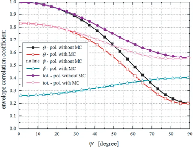
Figure 6. Envelope correlation coefficients for varying distances at ψ= 45◦ of θ and φ polarizations with or without mutual coupling (MC).
Figure 7. Envelope correlation coefficients for varyingψangles at 0.3λdistance ofθandφpolarizations with or without mutual coupling (MC).
coefficients forθpolarization are slightly lower than those without MC, particularly for low slant angles. For φ polarization, the correlation coefficient increases in accordance with increased slant angles (ψ) because φ polarization gain pattern of the antenna 2 increases due to the increased slant angle (ψ) as described in Eq. (6b). Total polarization component with MC is also similar to the θ polarization results; however, it increases at increased slant angles due to the effects of φpolarization components. Therefore, the analysis of the envelope correlation must also consider the polarization characteristics in accordance with the slant angle.
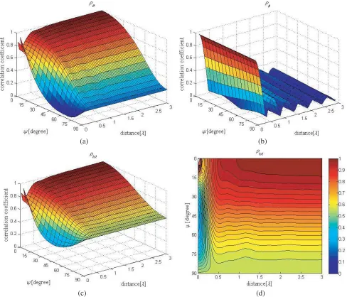
Three-dimensional envelope correlation coefficients for varying ψ angles and antenna distances of θ, φ, and total polarizations with MC are presented in Fig. 8. The result of θ polarization correlation gradually converges to a constant value according to the antenna distance and decreases according to the increasing slant angle ψ over a distance of 0.5λ. The minimum point of correlation is located at approximately ψ = 70◦ and below a distance of 0.5λ. The result of the φ polarization follows the sinc function for each slant angle. After combining both polarization components, the total polarization
(a) (b)
(c) (d)
correlation coefficient follows the results presented in Figs. 8(c) and (d). The minimum point of the total polarization correlation is located atψ= 50◦ andd= 0.05λ. Furthermore, low correlation region below the value of 0.5 is located at 25◦ ≤ψ≤80◦ andd≤0.3λ. Thus, the total polarization correlation result is strongly related to both θand φpolarization components. Therefore, both polarization components must be considered in the correlation analysis.
This subsection assumes a uniform and isotropic multipath propagation environment and the same incoming ratio of polarizations using rich scattering channels. For more realistic propagation channel environments, various angular density functions and XPDs are considered in Subsection 3.2. Capacity is a criterion used to estimate the performance of the communications system. The channel capacity strongly depends on the antenna correlations. The capacity can be estimated using two antenna correlation and signal-to-noise ratio (SNR) [40]; it is expressed as follows:
Cap.= log2
1 +SN R+
1− |ρ|2 SN R 2
2
[bits/s/Hz], (14)
where ρ is the correlation coefficient. The capacity decline with high SNR is not significant at low correlation; however, when the correlation is high, it is steep. The capacities estimated using the calculated correlation coefficients with slant angles (ψ) and antenna distances are indicated in Fig. 9. The maximal capacity region is located at 30◦≤ψ≤70◦ andd≤0.3λ.
Figure 9. Estimated capacity using the calculated correlation coefficients according to the slant angles and antenna distances.
Figure 10. Spherical coordinates for antenna geometry and angular density functions of incoming waves.
3.2. Various Propagation Channel Environments
Gaussian model Laplacian model Double exponent model θ 2 , 2 , 2 ,, /2π V H V H m
p A e
− σ θ φ θ,φ − = 2 − , 2 V H σ − ,,
XPD 5 [dB],
10 , 15
v h v,h
m σ
= =
(θ)
pθ,φ(φ) =Aθ,φ
( ) 2
2
2σV,H
( )θ−mV,H pθ,φ(θ)=A eθ,φ
/2π
pθ,φ (φ) =Aθ,φ
pθ,φ(θ)=A eθ,φ
/2π
pθ,φ (φ) =Aθ,φ
θ−mV,H
ο = ο
,,
XPD 5 [dB],
10 , 15
v h v,h
m σ
=
= ο = ο
,,
XPD 5 [dB],
10 , 15
v h v,h
m σ
=
= ο = ο
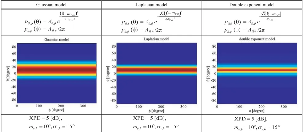
Figure 11. Statistical distribution models of incoming waves with angular density functions for each polarization and their characteristic factors for urban propagation channel models.
and double exponent models. The angular density functions of the statistical channel models with their characteristic factors are indicated in Fig. 11. Then, the statistical channel models are investigated in correlation analyses of the two skewed dipoles.
The correlation coefficient can be calculated using the gains of each antenna as
ρθ(ϕ) =
4π
Gemb1,θ(ϕ)pθ(ϕ) Gemb2,θ(ϕ)pθ(ϕ) ∗
dΩ
4π
Gemb1,θ(ϕ)pθ(ϕ) Gemb1,θ(ϕ)pθ(ϕ) ∗
dΩ
4π
Gemb2,θ(ϕ)pθ(ϕ) Gemb2,θ(ϕ)pθ(ϕ) ∗
dΩ
, (15a)
ρtot =
4π
Gemb1,θ pθ Gemb2,θ pθ ∗
+XP D2·
Gemb1,ϕpϕ Gemb2,ϕpϕ ∗
dΩ
4π
Gemb1,θ pθ Gemb1,θ pθ ∗
+XP D2·
Gemb1,ϕpϕ Gemb1,ϕpϕ ∗
dΩ
4π
Gemb2,θ pθ Gemb2,θ pθ ∗
+XP D2·
Gemb2,ϕpϕ Gemb2,ϕpϕ ∗
dΩ
. (15b)
The effective gains of each statistical propagation channel model are varied by the given embedded beam pattern and each angular density function forθ,φ, and total polarizations in the correlation coefficient calculation. Vaughan et al. [1] considered the complex electric field patterns ofθandφpolarizations and their angle of arrival probability distributions, which are the power density functions of the incoming θ and φpolarized waves, in order to calculate the total polarization correlations. Thus, the first order XPD is used to connect both polarization correlations. However, Kildal and Rosengren [36] applied the embedded gain patterns to calculate the correlation coefficient; thus, the angular density functions for each embedded gain pattern are also considered. Therefore, the square of the XPD is adopted in connection with both polarization correlations through effective power gains. Then, the proposed correlation coefficients can be written as Eqs. (15a), (15b) where pθ and pφ are the angular density functions for the θand φpolarizations and XPD is the power ratio Pθ/Pφ.
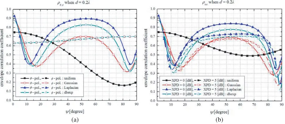
polarization correlation point for urban channel models is observed at 10◦ ≤ψ≤20◦ and 80◦ ≤ψ≤85◦ approximately, and these differed from the uniform distribution model. The results are related to the mean incident angle of a channel model and its standard deviation. The φ polarization correlations are the same for all channel models. Although various channel models are applied, the φpolarization patterns does not change. The total polarization correlation coefficients for XPD = 0 dB are similar to the θ polarization correlations but are slightly decreased by the φ polarization component in 0 dB ratio of the XPD according to Eq. (15b). However, when XPD = 5 dB, the φpolarization components strongly effect on the total polarization correlations compared to XPD = 0 dB. Thus, the shapes of the total correlation coefficient are lowered and the minimum correlation points are also changed to regions at 10◦ ≤ ψ ≤ 15◦ and 85◦ ≤ ψ ≤ 90◦ approximately, as shown in Fig. 12(b). Finally, the total correlation coefficient strongly depended on the environment variables such as the angular density function and XPD in the specific environment.
(a) (b)
Figure 12. (a) Envelope correlation coefficients for θ and φ polarizations at an antenna distance of 0.2λwith varyingψangles for XPD = 0 dB and (b) total polarization for XPD = 0 and 5 dB for various propagation environments.
Next, the envelope correlation coefficients forθ,φ, and total polarizations with MC atψ= 45◦ for varying antenna distances are shown in Fig. 13. The correlation coefficients for theθandφpolarizations for various propagation channel models are presented in Fig. 13(a). The minimum θ polarization correlation points for the urban channel models are observed at 1λ ≤ d≤ 1.25λ, approximately, and these differ from the uniform distribution model. Theφpolarization correlation coefficients are similar to the sinc function solutions for all applied channel models. The total polarization correlation coefficients for XPD = 0 dB are similar to theθpolarization correlations but decreas slightly with theφpolarization component with the same ratio of theθpolarization. When XPD = 5 dB, theφpolarization component has a significantly effect on the total polarization correlation. Thus, the total polarization correlation coefficients changes similarly to theφpolarization correlation as indicated in Fig. 13(b). Moreover, the minimum correlation area also changed to the d= 0.5∼0.75λregions.
(a) (b)
Figure 13. (a) Envelope correlation coefficients for θ and φ polarizations at ψ = 45◦ with varying antenna distances for XPD = 0 dB and (b) total polarization with XPD = 0 and 5 dB for various propagation environments.
(a) (b)
Figure 14. Three-dimensional correlation coefficients for varying ψ angles and antenna distances of total polarization of Laplacian distributions for (a) XPD = 0 dB and (b) XPD = 5 dB.
antenna distances is considerably widened. Despite the two different XPDs, there are other minimum areas. That is, the points near an antenna distance of 0.2λ and angles of ψ = 10◦ and 85◦ are the optimal regions for all propagation channel environments and various XPDs. These points can be slightly changed by different channel models and XPDs. Consequently, these are strong points for optimal geometric design in urban propagation channel environments.
(a) (b)
Figure 15. Envelope correlation coefficients for varying distances at ψ= 45◦ of total polarization for various XPDs in (a) a uniform distribution and (b) a Laplacian distribution.
Laplacian distribution [41, 42]. The shapes of the total correlation coefficients are transformed from θ polarization correlations to φ polarization correlations using Eq. (15b) from lower to higher values of XPDs. Therefore, the polarizations of the transmission and reception waves are important factors in the diversity antenna correlation as well as the polarization characteristics of the designed antenna in a specific environment.
4. CONCLUSION
In this work, the correlation coefficients of antenna diversity are theoretically analyzed using skewed dipole arrays with polarization characteristic. A simple mutual coupling estimation method for two skewed dipoles is proposed using the effective length vector (ELV) method. Furthermore, the embedded beam pattern is calculated using the estimated mutual impedance, and the mutually coupled correlation coefficient is effectively derived. The correlation is significantly affected by the polarization characteristics of the embedded beam pattern. For the lowest correlation coefficient, the gain patterns between the two antennas should be as different as possible. The mutual coupling between the antennas may cause the pattern to be changed, and the degree of correlation may be lowered. It is generally known to have the lowest correlation at half wavelength distances, but it is limited toφpolarization. Therefore, depending on the structure of the two antennas, it is advantageous to place theθpolarization antenna as close as possible, and to have a low correlation with the half-wave distance of theφpolarization antenna. And the envelope correlation coefficients are analyzed in various propagation channel environments using statistical models with respective angular density functions and cross polarization discriminations (XPDs). From these analyses, the optimal geometric structure of two skewed dipoles is proposed for low correlation in a specific propagation channel considering the polarization characteristics and the environment variables.
ACKNOWLEDGMENT
REFERENCES
1. Vaughan, R. G. and J. B. Andersen, “Antenna diversity in mobile communications,”IEEE Trans.
Veh. Technol., Vol. 36, No. 4, 149–172, Nov. 1987.
2. Vaughan, R. G., “Polarization diversity in mobile communications,” IEEE Trans. Veh. Technol., Vol. 39, No. 3, 177–186, Aug. 1990.
3. Dietrich, Jr., C. B., K. Dietze, J. R. Nealy, and W. L. Stutzman, “Spatial, polarization, and pattern diversity for wireless handheld terminals,”IEEE Trans. Antennas Propagat., Vol. 49, No. 9, 1271– 1281, Sep. 2001.
4. Clarke, R. H., “A statistical theory of mobile radio reception,” Bell Syst. Tech. J., Vol. 47, No. 6, 957–1000, Jul.–Aug. 1968.
5. Tse, D. and P. Viswanath, Fundamentals of Wireless Communication, Cambridge Univ. Press, 2005.
6. Saraswat, R. K. and M. Kumar, “Miniaturized slotted ground UWB antenna loaded with metamaterial for WLAN and WiMAX applications,” Progress In Electromagnetics Research B, Vol. 65, 65–80, 2016.
7. Saraswat, R. K. and M. Kumar, “A frequency band reconfigurable UWB antenna for high gain applications,” Progress In Electromagnetics Research B, Vol. 64, 29–45, 2015.
8. Andrews, R. A., P. P. Mitra, and R. de Carvalho, “Tripling the capacity of wireless communications using electromagnetic polarization,”Nature, Vol. 409, 316–318, 2001.
9. Derneryd, A. and G. Kristensson, “Signal correlation including antenna coupling,” Electron. Lett., Vol. 40, No. 3, 157–159, Feb. 2004.
10. Blanch, S., J. Romeu, and I. Corbella, “Exact representation of antenna system diversity performance from input parameter description,” Electron. Lett., Vol. 39, No. 9, 705–707, 2003. 11. Valenzuela-Vald´es, J. F., M. A. Garc´ıa-Fern´andez, A. M. Mart´ınez-Gonz´alez, and D. S´
anchez-Hern´andez, “The role of polarization diversity for MIMO systems under Rayleigh-fading environments,”IEEE Antennas Wireless Propagt. Lett., Vol. 5, 534–536, 2006.
12. Valenzuela-Vald´es, J. F., A. M. Mart´ınez-Gonz´alez, and D. S´anchez-Hern´andez, “Estimating combined correlation functions for dipoles in Rayleigh-fading scenarios,” IEEE Antennas Wireless
Propagat. Lett., Vol. 6, 349–352, 2007.
13. Valenzuela-Vald´es, J. F., M. A. Garc´ıa-Fern´andez, A. M. Mart´ınez-Gonz´alez, and D. S´ anchez-Hern´andez, “Evaluation of true polarization diversity for MIMO systems,”IEEE Trans. Antennas
Propagat., Vol. 57, No. 9, 2746–2755, Sep. 2009.
14. Taga, T., “Analysis for mean effective gain in mobile antennas in land mobile radio environments,”
IEEE Trans. Veh. Technol., Vol. 39, No. 2, 117–131, May 1990.
15. Vaughan, R. G., “Switched parasitic elements for antenna diversity,” IEEE Trans. Antennas
Propagat., Vol. 47, No. 2, 399–405, Feb. 1999.
16. Boyle, K., “Radiation patterns and correlation of closely spaced linear antennas,” IEEE Trans.
Antennas Propagat., Vol. 50, No. 8, 1162–1165, Aug. 2002.
17. Hui, H. T., W. T. O. Yong, and K. B. Toh, “Signal correlation between two normal-mode helical antennas for diversity reception in a multipath environment,” IEEE Trans. Antennas Propagat., Vol. 52, No. 2, 572–577, Feb. 2004.
18. Hallbj¨orner, P., “The significant of radiation efficiencies when using S-parameters to calculate the received signal correlation from two antennas,” IEEE Antennas Wireless Propagat. Lett., Vol. 4, 97–99, 2005.
19. Andersen, J. B. and B. K. Lau, “On closely coupled dipoles in a random field,” IEEE Antennas
Wireless Propagat. Lett., Vol. 5, 73–75, 2006.
21. Hsieh, P. C. and F. C. Chen, “A new spatial correlation formulation of arbitrary AoA scenarios,”
IEEE Antennas Wireless Propagat. Lett., Vol. 8, 398–401, 2008.
22. King, H. E., “Mutual impedance of unequal length antennas in echelon,” IRE Trans. Antennas
Propagat., Vol. 5, No. 3, 306–313, Jul. 1957.
23. Chang, V. W. H. and R. W. P. King, “On two arbitrarily located identical parallel antennas,”
IEEE Trans. Antennas Propagat., Vol. 16, No. 3, 309–317, May 1968.
24. Janaswamy, R., “A simplified expression for the self/mutual impedance between coplanar and parallel surface monopoles,” IEEE Trans. Antennas Propagat., Vol. 35, No. 10, 1174–1176, Oct. 1987.
25. K¨oksal, A. and J. F. Kauffman, “Mutual impedance of parallel and perpendicular coplanar surface monopoles,”IEEE Trans. Antennas Propagat., Vol. 39, No. 8, 1251–1256, Aug. 1991.
26. King, R. W. P. and C. W. Harrison, Jr, “The receiving antenna,” Proc. IRE, Vol. 32, 18–49, Jan. 1944.
27. Richmond, J. H. and N. H. Geary, “Mutual impedance between coplanar-skew dipoles,” IEEE
Trans. Antennas Propagat., Vol. 18, 414–416, May 1970.
28. Richmond, J. H., “Coupled linear antennas with skew orientation,” IEEE Trans. Antennas
Propagat., Vol. 18, 694–696, Mar. 1970.
29. Han, J. H. and N. H. Myung, “Exact and simple calculation of mutual impedance for coplanar-skew dipoles,” Electron. Lett., Vol. 48, No. 8, 423–425, Apr. 2012.
30. Richmond, J. H. and N. H. Geary, “Mutual impedance of nonplanar-skew sinusoidal dipoles,”IEEE
Trans. Antennas Propagat., Vol. 23, 412–414, May 1975.
31. Chuang, C. W., J. H. Richmond, N. Wang, and P. H. Pathak, “New expressions for mutual impedance of nonplanar-skew sinusoidal monopoles,” IEEE Trans. Antennas Propagat., Vol. 38, No. 2, 275–276, Feb. 1990.
32. Liu, K., C. A. Balanis, and G. C. Barber, “Exact mutual impedance between sinusoidal electric and magnetic dipoles,” IEEE Trans. Antennas Propagat., Vol. 39, No. 5, 684–686, May 1991. 33. Schmidt, K. E., “Simplified mutual impedance of nonplanar skew dipoles,”IEEE Trans. Antennas
Propagat., Vol. 44, No. 9, 1298–1299, Sep. 1996.
34. Han, J. H., W. Y. Song, K. S. Oh, and N. H. Myung, “Simple formula and its exact analytic solution of mutual impedance for nonplanar skew dipoles,” Progress In Electromagnetics Research, Vol. 132, 551–570, 2012.
35. Svantesson, T. and A. Ranheim, “Mutual coupling effects on the capacity of multielement antenna systems,”Proc. IEEE Int. Conf., Acoustics, Speech, and Signal Processing, 2485–2488, 2001. 36. Kildal, P. S. and K. Rosengren, “Electromagnetic analysis of effective and apparent diversity gain
of two parallel dipoles,”IEEE Antennas Wireless Propagat. Lett., Vol. 2, 9–13, 2003.
37. Rosengren, K. and P. S. Kildal, “Radiation efficiency, correlation, diversity gain and capacity of a six-monopole antenna array for a MIMO system: Theory, simulation and measurement in reverberation chamber,” Proc. Inst. Elect. Eng. on Microwaves, Antennas and Propagation, Vol. 152, No. 1, 7–16, 2005.
38. Balanis, C. A.,Antenna Theory, Analysis, and Design, Wiley, 1982.
39. Li, X. and Z. P. Nie, “Mutual coupling effects on the performance of MIMO wireless channels,”
IEEE Antennas Wireless Propagat. Lett., Vol. 3, 344–347, 2004.
40. Loyka, S. L., “Channel capacity of two antenna BLAST architecture,” Electron. Lett., Vol. 35, No. 17, 1421–1422, Aug. 1999.
41. Kalliola, K., K. Sulonen, H. Laitinen, O. Kivek¨as, J. Krogerus, and P. Vainikainen, “Angular power distribution and mean effective gain of mobile antenna in different propagation environments,”
IEEE Trans. Veh. Technol., Vol. 51, No. 5, 823–838, Sep. 2002.
42. Ando, A., T. Taga, A. Kondo, K. Kagoshima, and S. Kubota, “Mean effective gain of mobile antennas in line-of-sight street microcells with low base station antennas,”IEEE Trans. Antennas