The Reactive Simulatability (RSIM) Framework
for Asynchronous Systems
∗Michael Backes†, Birgit Pfitzmann, and Michael Waidner‡
Abstract
We define reactive simulatability for general asynchronous systems. Roughly, simulata-bility means that a real system implements an ideal system (specification) in a way that preserves security in a general cryptographic sense. Reactive means that the system can interact with its users multiple times, e.g., in many concurrent protocol runs or a multi-round game. In terms of distributed systems, reactive simulatability is a type of refinement that preserves particularly strong properties, in particular confidentiality. A core feature of reactive simulatability iscomposability, i.e., the real system can be plugged in instead of the ideal system within arbitrary larger systems; this is shown in follow-up papers, and so is the preservation of many classes of individual security properties from the ideal to the real systems.
A large part of this paper defines a suitable system model. It is based on probabilistic IO automata (PIOA) with two main new features: One is generic distributed scheduling. Important special cases are realistic adversarial scheduling, procedure-call-type scheduling among colocated system parts, and special schedulers such as for fairness, also in combi-nations. The other is the definition of the reactive runtime via a realization by Turing machines such that notions like polynomial-time are composable. The simple complexity of the transition functions of the automata is not composable.
As specializations of this model we define security-specific concepts, in particular a sep-aration between honest users and adversaries and several trust models.
The benefit of IO automata as the main model, instead of only interactive Turing ma-chines as usual in cryptographic multi-party computation, is that many cryptographic sys-tems can be specified with an ideal system consisting of only one simple, deterministic IO automaton without any cryptographic objects, as many follow-up papers show. This enables the use of classic formal methods and automatic proof tools for proving larger distributed protocols and systems that use these cryptographic systems.
Keywords: security, cryptography, simulatability, formal methods, reactive systems, compos-ability, probabilistic IO automata, distributed polynomial time
1
Introduction
In this paper we present the reactive simulatability (RSIM) framework for general asynchronous systems. More precisely, we present the definition of reactive simulatability and a general reactive asynchronous system model as a basis for this definition and many other general security definitions and theorems.
∗A preliminary version of this paper appeared as part of a paper by Pfitzmann and Waidner at IEEE
Sym-posium on Security and Privacy, Oakland, May 2001.
†Saarland University, Saarbr¨ucken, Germany, [email protected]. Work done while at IBM Zurich Research
Laboratory, R¨uschlikon, Switzerland.
1.1 The Idea of Reactive Simulatability
The basic idea of reactive simulatability, sometimes abbreviated as RSIM, is to define under what conditions one system, typically a real cryptographic system, securely implements another system, typically a much simpler specification called ideal system. Roughly, we define that this is true if everything that can happen to the honest users of the real system, with strong real adversaries, can also happen to the same honest users if they use the ideal system, where adversaries do not occur or at least have far less power. What happens to the users includes the aspect of the adversary’s knowledge about the users’ behavior and secrets.
Definitions of a real system implementing a specification are well-known in the field of distributed systems and often called refinement; however, normal refinement does not retain confidentiality properties and is therefore not suitable for most security systems, in particular for most cryptographic systems and protocols. For instance, if one defines an ideal secure channel essentially as a black box where messages are put in on one side and come out on the other side, normal notions of correct implementation by a distributed system allow that intermediate parties learn the messages. For security and cryptography, however, this should not happen if the ideal secure channel gives no information to such parties.
In cryptography, a suitable notion of secure implementation, typically called simulatability, was already defined for ideal systems (specifications) that are just functions: each party makes one input at the beginning and obtains one output at the end. Essentially, we extend this notion to reactive systems, i.e., systems where parties may make inputs and obtain outputs at many different times. Examples of reactive cryptographic systems are multi-round auctions, protocols with many concurrent sessions, and untraceable electronic cash systems because whether a payment succeeds depends on prior cash withdrawal actions. For all these systems one requires confidentiality properties, so that the relation between a real system and a specification cannot only be the classical refinement of distributed systems. Reactive simulatability makes the real-and-ideal system specification technique available for such types of systems.
An important property of reactive simulatability iscomposability. Roughly this means that a larger system can be defined based on the specification of a subsystem, in other words with an ideal subsystem, and then the real subsystem can be plugged in instead without causing any significant difference. The notion of “no significant difference” is again reactive simulatability. Composability is generally required of refinement relations in distributed systems. The idea of reactive simulatability has also become known as universal composability (UC) for such properties. (We describe the history of these terms and theorems in Section 1.7.) Reactive simulatability also offers property preservation, i.e., if one proves certain important properties of an ideal system, then they also hold for the real system. An example of such a property is that the participants in a payment system cannot spend more money than they put in initially or received. Such properties are not always trivial to show for an ideal system, but usually very much easier than if one had to do it directly for the real system. However, for length reasons of this first journal version with detailed definitions, we do not prove any composition and property preservation theorems here although the first ones were in the corresponding conference publication.
1.2 Link to Formal Methods and Tool-Supported Proofs
adversaries, polynomial-time considerations, and error probabilities.
Besides this general motivation, a specific motivation for defining reactive simulatability was that it offers an important link between cryptography and formal methods, in particular automated proof tools such as model checkers and theorem provers. Interest in such a link can be justified from both prior cryptographic protocol proofs and from prior tool-supported proofs of security protocols: The cryptographic motivation is essentially the limit of human stamina when dealing with the many different sequences of actions occurring in executions of even relatively small protocols. The tool-supported proof motivation is the prior lack of demonstrated soundness with respect to real cryptography. We now discuss this in more detail. Typical cryptographic proofs are reductions between the security of an overall system under consideration and the security of the cryptographic primitives used: One shows that if one could break the overall system, one could also break one of the primitives with respect to its cryptographic definition, e.g., adaptive chosen-message security for signature schemes. In principle, these proofs are as rigorous as typical proofs in mathematics. In practice, however, human beings are extremely fallible with such proofs when protocols are concerned. This is mainly due to the distributed-systems aspects of the protocols. It is well-known from non-cryptographic distributed systems that many wrong protocols have been published even for very small problems. Hand-made proofs are highly error-prone because following all the different orders of interleaving of the actions of different participants is extremely tedious. Humans tend to take wrong shortcuts and do not want to proof-read such details in proofs by others. If the protocol contains cryptography, the situation is even worse: Already a rigorous definition of the goals and of the protocol itself gets more complicated, and there was previously no general framework for this. Compared with protocol proofs outside security, which are mostly for trace properties, i.e., properties of individual runs, confidentiality properties are more complex because they are properties of entire probability spaces of runs. Moreover, in principle the complexity-theoretic reduction has to be carried out across all the different interleavings, and it is not at all trivial to do this rigorously. In consequence, there are very few real cryptographic proofs of larger protocols, and several times supposedly proven, relatively small systems were later broken. Hence tool support should be very welcome, at least for the tedious distributed-system aspects.
In fact, work on tool-supported proofs of cryptographic protocols started as early as work on computational cryptographic definitions and proofs. Tools mean model checkers and automatic theorem provers; initially mostly special-purpose for security protocols, nowadays mostly spe-cializations of more general tools. However, for a very long time all these proofs were based on idealized abstractions of cryptographic primitives, almost always by representing cryptographic operations as operators of a term algebra with cancellation rules, so-called Dolev-Yao models. For instance, public-key encryption is represented by operatorsEfor encryption and D for de-cryption with one cancellation rule,D(E(m)) =m for all m. Encrypting a message m twice in a Dolev-Yao model does not yield another message from the basic message space but the term
clearly an unsatisfactory situation, and artificial counterexamples can be constructed.
The main use of reactive simulatability in the context of linking cryptography and formal methods in a sound way is that it can be the gauge for deciding whether an idealization is securely realized by a specific cryptographic implementation, or even realizable by any such implementation. One specific goal, achieved later, was to apply this gauge to Dolev-Yao models. However, the approach is not at all limited to Dolev-Yao models – many possible ideal systems used as specifications for cryptographic systems are quite simple and can thus be encoded into existing proof tools, so that those proof tools can be used when larger systems are proved that use these cryptographic systems.
1.3 Requirements on the System Model
The first obstacle to defining reactive simulatability was that there was no system model, i.e., a model of protocol participants and how they interact, that combined all the features we desire:
• Allowing reactive systems.
• Enabling system definitions that are not encumbered by Turing machine details, in par-ticular for ideal systems and with the aim of encodings into some current proof tools.
• Allowing run-time considerations, because most cryptographic systems are only secure against computationally bounded adversaries. We also desire composability of runtimes; in particular the combination of polynomial-time entities should be polynomial again. This is particularly important in compositions, where the protocol machines of higher layers become the users of the lower-layer systems. Users also have to be polynomially bounded so that an adversary cannot offload computations to them in active attacks.
• Asynchronous systems with a sufficiently flexible scheduling model that all typical cases can be represented. A scheduling model defines how it is determined in which order different actions, in particular of different distributed entities, occur. In particular, we want to allow:
– scheduling by the adversary with realistic information;
– procedure-call-style scheduling for colocated components; this occurs in particular in compositions, when a higher-layer entity uses a lower-layer entity in the same location; and
– restricted scheduling, e.g., fair schedulers for liveness-style considerations (i.e., re-quirements that something should happen, possibly within restricted time), or for encoding synchronous systems.
• Independence of trust models. This means that the core system model should not fix issues like what computational power an adversary has, how it can corrupt participants, and how it can manipulate messages on channels. There are many variants of this, and we want to be able to express them all.
General system model
(Section 3) Machines (with, e.g., clock
ports and length bounds)
Collections Runs, views
Security-related system model (Sections 4, 5)
Structure = collection + service ports Systems
Security parameter
Reactive simulatability (general, universal, blackbox / perfect, statistical, computational)
Static part (topology) Dynamic part (execution)
Italics: explanatory words
Straight: Defined terms
Poly, weakly poly
Special cases or patterns (Section 6)
Some specific trust models: static and adaptive adversaries; secure, authentic, insecure channels
Configuration = structure + A + H
Turing machine realization
Figure 1: Overview of our layers of definitions
examples of trust models, mainly for real systems, in particular for static and dynamic adver-saries and for channels with different types of security. These layers and the main definitions we make on each layer are surveyed in Figure 1. The first four requirement above all refer to the lowest layer. Some details of these requirements may become clearer when we explain how we address them.
1.4 Asynchronous System Model with General Distributed Scheduling and
Runtimes
We use an IO automata model as our core model, in other words state-transitions systems that specify the next output and state for every given input and state. Given the importance of probabilism in cryptography we need probabilistic IO automata (PIOAs). We did not choose interactive Turing machines as the core model, although this was normal at that time in cryp-tography, because of our requirement that ideal systems, if they are simple in principle, should be easy to encode into existing proof tools from our concrete specification. IO automata are the typical basis for encoding distributed systems into the specification languages of standard the-orem provers. Furthermore, most formal languages (i.e., with fully fixed syntax) for distributed systems have some state-transition system as their semantics. Informally also cryptography has often used IO automata, because nobody actually specifies cryptographic protocols as Turing machines; the specifications in articles are much closer to IO automata as soon as they go beyond simple arrow pictures.
One novelty is that we allow essentially arbitrary scheduling schemes. The basis of schedul-ing is message delivery: In an asynchronous system, a message does not arrive immediately at its recipient, but may be held up in the network. In our generic distributed scheduling, one can designate for each connection which party decides about the arrival of the messages on this connection; we call this party thescheduler of this connection. Thus in particular we can model the special cases required above:
• We can let the adversary schedule everything by making it the scheduler of all connections.
• Or a separate scheduler can schedule everything, or only certain connections (e.g., secure ones) while the adversary schedules others.
While the generic distributed scheduling allows many more variants, these three (in particular combinations of the first and the second) are mostly used in subsequent work.
For computational complexity, the easiest option would be to consider the complexity of the state-transition function of the IO automata. The complexity of functions is well-defined and we would never need to mention the underlying bit-level model like Turing machines, in particular if we concentrate on notions like polynomial-time that are robust against small model variations. However,polynomial-time transitions do not even lead to overall polynomial runtime when such a machine runs essentially alone: For instance, such a machine might double the size of its current state in each transition; thus it can use time exponential in its initial state size after a linear number of transitions with one-bit inputs. In a medium notion, which we call
weakly polynomial-time, the runtime of the machine is polynomial in the overall length of its inputs and its initial state. A weakly polynomial-time machine is a permissible adversary when interacting with a cryptographic system which is in itself polynomially bounded; i.e., this seems to be the weakest useful definition. However, this notion does not compose: Several weakly polynomial-time machines together can become too powerful. E.g., each new output may be twice as long as the inputs so far. Then with a linear number of interactions, these machines can use time exponential in the size of their initial states.
Hence we define polynomial-time machines as those that only need time polynomial in their initial state size, independent of all inputs. This notion is composable.
We nevertheless use weakly polynomial-time machines sometimes, because many function-alities are naturally weakly polynomial-time and not naturally polynomial-time.
We made one further addition to individual machines compared with other I/O automata models, in order to enable machines to have polynomial runtime independent of their environ-ment without being automatically vulnerable to denial-of-service attacks by long messages: We allow state-dependentlength bounds on the inputs that a machine will read from each channel.
1.5 Security-Related System Model
Reactive simulatability is about systems, users, and adversaries: If the same honest users use either the real or the ideal system, they shouldn’t notice a difference, even though the real system typically gives an adversary much more power than the ideal system. Hence we have to define users and adversaries. The general system model sketched in Section 1.4 simply allows “open” systems that can interact with some environment. The user-adversary distinction is essential but quite simple: We split the interaction opportunities (later called ports; also think of them as unattached connections) into some for the honest users and others for the adversary. We call the formerservice ports. We call such an open system with a split into service ports and others astructure, and if we augment it by an honest user and an adversary in the designated way, we call it aconfiguration.
We also define systems as sets of structures; this is the general provision for trust models which allow that instead of one structure intended by a designer (e.g., with n machines for n
A H
M1 M2
S
A' H
TH
S
Service ports
Honest users
(Real) adversary (Real) machines
and connections
(Ideal) machine(s), here one "trusted
host”
(Ideal) adversary (The same)
honest users
A Sim
Connection, e.g., for chosen-message
attacks
Simulator
In the blackbox
case
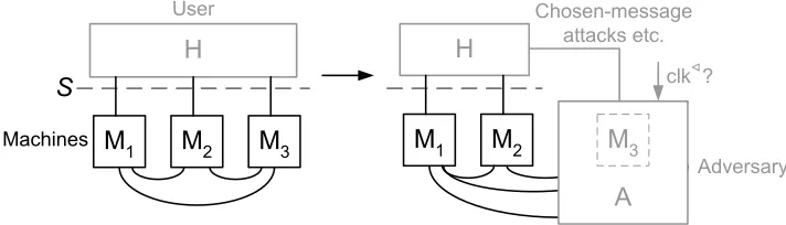
Figure 2: Overview of reactive simulatability
1.6 Reactive Simulatability Variants
We have already introduced reactive simulatability, the main goal of our definitions, in Sec-tion 1.1. Figure 2 illustrates it, including typical identifiers that we use for various parts. The left half illustrates a real system. Here it consists of a structure with only two machines (PIOAs)
M1 and M2. An entirety of honest users H uses it via the service ports, and an adversary A
interacts both with the two “normal” machines and the honest users. This is compared with the ideal system on the right side. In this example, the structure in the ideal system consists of just one machine, which we often call THfor “trusted host” (corresponding to the intuition that a trusted host would simply do for the participants what in reality they have to do via a complex cryptographic protocol). Formally there is no difference between ideal and real systems in our model; this is useful in compositions and other multi-part security proofs. The same honest users use the ideal structure via the same service ports, and there may again be an adversary
A′.
We define reactive simulatability in several variants: In one dimension, we vary the order of quantifiers in the statement that for all honest users H and all adversaries A on the real system, there should be an adversary A′ on the ideal system that achieves the same effects. What we just wrote isgeneral reactive simulatability (GRSIM). If the ideal adversary does not depend on the honest users (only on the real adversary and of course the system), we speak of
universal reactive simulatability (URSIM), i.e., then the quantifier order is∀A∃A′∀H. If the ideal adversary consists of a fixed part that uses the real adversary as a blackbox, we speak ofblackbox reactive simulatability (BRSIM)and call the fixed partsimulator. In another dimension, we have a perfect, a statistical, and a computational variant, depending on computational restrictions and the degree of similarity we require between the real and the ideal system.
1.7 Prior Work
face of continuous external inputs, do not occur in the function-evaluation case, since function evaluation is non-reactive. A composition theorem for non-reactive simulatability was proven in [38].
The idea of simulatability was subsequently also used for specific reactive problems, e.g., [55, 32, 44], without a detailed or general definition. In a similar way it was used for the construction of generic solutions for large classes of reactive problems [57, 56, 61] (usually yielding inefficient solutions and assuming that all parties take part in all subprotocols). A reactive simulatability definition was first proposed (after some earlier sketches, in particular in [57, 90, 38]) in [61]. It is synchronous, covers a restricted class of protocols (straightline programs with restricted operators, in view of the constructive result of this paper), and for the information-theoretic case only, where quantification over input sequences can be used instead of active honest users.
We first presented a synchronous version of a general reactive system model and reactive simulatability in [91]. The report version also contains further variants of the reactive simu-latability definitions with proofs of equivalence or non-equivalence that are likely to carry over to the asynchronous case.
After that, and later but independently to the conference version [92] of the current paper, an asynchronous version of a general reactive model and reactive simulatability was also given in [39]. The model parts that were relatively well-defined seem to us a strict subset of our model: The system correspond to our “cryptographic systems with adaptive adversaries” in Section 6.3, always with polynomial-time users and adversaries. The entities are defined as Turing machines only, i.e., there is no explicit abstraction layer like our IO automata. The simulatability definition corresponds to the universal case of ours. Besides the model, the paper contains a composition theorem which was more general than ours at that time, while we had a property preservation theorem. Here the term UC (universal composability) was coined which is nowadays also widely used for the general idea of reactive simulatability or the definitions. (The paper also contains some sketches, while we had decided to only publish parts that we had actually defined and proved.)
The first rigorous model for reactive systems that covers cryptography, i.e., probabilistic and polynomial-time aspects, was presented in [73, 74]. It is based on π-calculus and uses formal language characterizations of polynomial time. The notion of security is observational equivalence. This is even stronger than reactive simulatability because the entire environment (corresponding to our users and adversary together) must not be able to distinguish the im-plementation and the specification. However, this excludes many abstractions, e.g., because a typical abstract specification is one machine and the real system is distributed with channel manipulation possibilities for the adversary, so that an adversary can already distinguish them by their structure. Correspondingly, the concrete specifications used essentially comprise the actual protocols including all cryptographic details. There was no tool support for the proofs at that time, as even the concrete specifications involved ad-hoc notations, e.g., for generating random primes.
Reductions as cryptographic proofs were introduced for cryptographic primitives in [35, 59, 100]. The best-known application to protocols is the handling of authentication protocols originating in [33]. Examples of later breaks of supposedly proven cryptographic systems are given in [89, 52, 63].
that there wasn’t even a definition for such a comparison under active attacks, and only reac-tive simulatability provided this later. Logics of belief for cryptographic protocol proofs were introduced in [36]. A semantics for such a model (in the sense of an execution semantics, still relying on a Dolev-Yao model for the cryptography) was first given in [3]. Careful study of this semantics shows that one needs hand-proofs of strong protocol properties before the logic applies; this is never done in practice. This is why we did not count breaks of protocols proven in such logics as counter-arguments against the Dolev-Yao models or proof tools relying on normal distributed-systems semantics.
IO automata were already used for security in [79]. There however, cryptographic systems are restricted to the usual equational specifications following a Dolev-Yao model [53], and the semantics is not probabilistic. Only passive adversaries are considered and only one class of users, called environment. The author actually remarks that the model of what the adversary learns from the environment is not yet general, and that general theorems for the abstraction from probabilism would be useful. Our model solves these problems.
So far we looked at prior security definitions. We now consider literature on system mod-els as such. Our IO automata are based on normal finite-state machines; deterministic and non-deterministic versions, also with infinite state, have been used widely throughout the dis-tributed protocol literature. Probabilistic IO-automata and execution models for them are defined in [94, 78, 98]. There the order of events is chosen by a probabilistic scheduler that has full information about the system. However, this can give the scheduler too much power in a cryptographic scenario. In cryptology, the typical understanding of asynchronous systems, closest to a rigorous definition in [37], is that the adversary schedules everything, but only with realistic information, in terms of both observations and computational capabilities. Recall that this is still an important special case in our model. We are sometimes asked why we do not just elaborate this case. However, there are situations where one definitely needs more benign scheduling or even some synchrony, as in our third special case (e.g., one may want to show liveness properties, but can only do so if one can model that messages are eventually delivered). As to local scheduling among system parts modeled as different automata but considered co-located, adversarial scheduling may often do no harm. However, having to prove it when one actually is considering a local situation, only defined as a composition, would just introduce unnecessary complications into the proof. Modeling only adversarial scheduling would remove the need to represent who schedules what, while the underlying model of asynchronous connec-tions would remain the same. Problems with purely adversarial scheduling were already noted in [74]; hence they schedule secure channels with uniform probability before adversary-chosen events. However, that introduces a certain amount of global synchrony. Furthermore, we do not require specific scheduling for all secure channels; they may be blindly scheduled by the adversary (i.e., without even seeing whether there are messages on the channel). For instance, this models the case where the adversary has a global influence on the relative network speed. There are also probabilistic versions of other detailed distributed-systems frameworks than IO automata, but apart from [73, 74] we are not aware of a prior one with polynomial-time considerations or any specific scheduling considerations for security.
We are also not aware of any prior model with a representation of both honest users and adversaries.
1.8 Subsequent Work
Secondly, it has a composition theorem that states that substituting a refined system (an implementation) for the original system (a specification) within a larger system is permit-ted [92]; compositionality of reactive simulatability in different settings has been investigapermit-ted in [39, 75, 24, 65, 51, 67, 70]. Thirdly, one can define computational versions of various secu-rity property classes and prove preservation theorems for them under reactive simulatability, in particular for integrity [91, 11], key and message secrecy [19], transitive and transitive non-interference [16, 15], i.e., absence of information flow, and classes of liveness properties [22, 10]. Various concrete cryptographic systems have been proven secure in the sense of reactive simulatability with respect to ideal specifications that are not encumbered with cryptographic details. This comprises secure message transmission [92, 46], key exchange [46], and group key agreement [96]. Under additional assumptions such as the existence of a common random reference string, this was extended to commitment schemes [43], oblivious transfer [48, 54], zero-knowledge proofs [43], and, more generally, any multi-party function evaluation [48]. Reactive simulatability also proved useful for lower-layer proofs, e.g., of reactive encryption and signature security from traditional (non-reactive) encryption and signature security within [92, 40] and [41, 25, 26], respectively, and of reactive Diffie-Hellman security within [96].
A particularly important ideal specification that has been proven to have a crypto-graphic realization secure in the sense of reactive simulatability is a specific Dolev-Yao model [23, 27, 17, 21], nowadays referred to as the BPW model. The BPW model offers a comprehensive set of Dolev-Yao-style operations for modeling and analyzing security protocols: both symmetric and asymmetric encryption, digital signatures, message authentication codes, as well as nonces, payload data and a list (pairing) operation. Proofs of the Needham-Schroeder-Lowe protocol [14], the Otway-Rees protocol [5], the Yahalom protocol [20], an electronic pay-ment protocol [7], and parts of public-key Kerberos [6] using the BPW model show that one can rigorously prove protocols based on this model in much the same way as with more traditional Dolev-Yao models. Weaker soundness notions for Dolev-Yao models such as integrity only or offline mappings between runs of the two systems, and/or allowing less general protocol classes, e.g., only a specific class of key exchange protocols, have been established in [82, 72, 45]. For these cases, simpler Dolev-Yao models and/or realizations can be used compared to [23].
Establishing reactive simulatability for concrete systems has proven an error-prone task if approached rather informally, as it requires to carefully compare various behaviors of an ideal specification with corresponding behaviors of the concrete system. We emphasize that it is quite easy to guess almost correct ideal specifications of cryptography systems; the major part of the work lies in getting the details right and making a rigorous proof. Several abstractions presented with less detailed proofs have been broken [63, 9] (where the first paper attributes another such attack to Damg˚ard). In order to establish reactive simulatability in a rigorous manner, the notion of a cryptographic bisimulation has been introduced in [23] and further extended in a sightly different framework in [42]. Cryptographic bisimulations are based on the notion of probabilistic bisimulations [71], which capture that two systems that are in related states and receive the same input will yield identically distributed states and outputs after they performed their next transition. Cryptographic bisimulations extend this notion with imperfections and, in the case of the BPW model, an embedded static information-flow analysis.
by reactive simulatability. Fully automated techniques for proving secrecy properties of security protocols based on the BPW model have been invented in [13] using mechanized flow analysis. In the wider field of linking formal methods and cryptography, there is also work on formulating syntactic calculi for dealing with probabilism and polynomial-time considerations directly, in particular [84, 85, 68, 50, 34]. This is orthogonal to the work of justifying Dolev-Yao models: In situations where Dolev-Yao models are applicable and sound, they are likely to remain im-portant because of the strong simplification they offer to the tools, which enables the tools to treat larger overall systems automatically than with the more detailed models of cryptography. Finally, the expressiveness of reactive simulatability, i.e., the question which cryptographic tasks can be assigned a suitable ideal functionality under which assumptions, has been investi-gated in a series of papers. It has been shown that several cryptographic tasks cannot be proven secure in the sense of reactive simulatability unless one makes additional set-up assumptions, e.g., by postulating the existence of a common random reference string. Among these tasks are bit commitment, zero-knowledge proofs, oblivious transfer [43], (authenticated) Byzantine agreement [76], classes of secure multi-party computation protocols [47], classes of functional-ities that fulfill certain game-based definitions [49], and Dolev-Yao style abstractions of XOR and hash functions [18, 28]. Other set-up assumptions to circumvent such impossibility results are to augment real and ideal adversaries with oracles that selectively solve certain classes of hard problems [93], to free the ideal adversary from some of its computational restrictions [29], or to impose constraints on the permitted honest users [8]. The price is either a narrower model tailored to a specific problem, sacrificing the transitivity of reactive simulatability and hence significantly complicating the modular construction of larger protocols, or providing only a limited form of compositionality.
1.9 Overview of this Paper
Section 2 introduces notation. Section 3 defines the general system model, i.e., machines, both their abstract version and their computational realization, and executions of collections of machines. Section 4 defines the security-specific system model, i.e., systems with users and adversaries. Section 5 defines reactive simulatability, i.e., our notion of secure refinement. Sec-tion 6 shows how to represent typical trust models, i.e., assumpSec-tions about the adversary, such as static threshold models and adaptive adversaries, with secure, authenticated and insecure channels. Section 7 concludes the paper.
2
Notation
Let Bool := {true,false}, and let N be the set of natural numbers and N0 := N∪ {0}. For an
arbitrary setA, let P(A) denote its powerset. Furthermore, letAn denote the set of sequences over Awith index setI ={1, . . . , n} forn∈N0,A∗ :=Sn∈N0A
n, and A∞the set of sequences
over A with index set I = N. We write a sequence over A with index set I as S = (Si)i∈I, where ∀i∈ I: Si ∈ A. Let◦ denote sequence concatenation, and () the empty sequence. Let
{()}denote the empty Cartesian product. For a sequenceS ∈A∗∪A∞we define the following notation:
• For a functionf:A→A′, letf(S) applyf to each element ofS, retaining the order.
• Let size(S) denote the length of S, i.e., size(S) := |I| if I is finite, and size(S) := ∞
• For l ∈ N0, let S⌈l (read “S restricted to l elements”) denote the l-element prefix of S,
and S[l] the l-th element ofS with the convention thatS[l] =ǫifsize(S)< l (for a fixed symbolǫ). We sometimes write Sl instead ofS[l] to increase readability.
• For a predicatepred: A→ Bool, let (S[i] ∈S |pred(S[i])) denote the subsequence of S
containing those elementsS[i] of S with pred(S[i]) =true, retaining the order.
We lift the restriction notation to finite sequences of sequences: For T = (T1, . . . , Tn) ∈(A∗ ∪ A∞)∗ andL= (L1, . . . , Ln)∈N∗0 with the samen∈N0, letT⌈L:= (T1⌈L1, . . . , Tn⌈Ln).
In the following, we assume that a finite alphabet Σ ⊇ {0,1,c,l,k} is given, where ∼
,!,?,↔,⊳6∈Σ. Then Σ∗denotes the strings over Σ. Letǫbe the empty string and Σ+:= Σ∗\{ǫ}. All notation for sequences can be used for strings, such as◦ for string concatenation, but ◦is often omitted.
For representing natural numbers and sequences of strings as strings, we assume a surjective function nat: Σ∗ → N with the convention nat(1) = 1, and a bijective function ι: (Σ∗)∗ →
Σ∗. We assume that standard operations are efficiently (polynomial-time) computable in these encodings; concretely we need this for inverting the function ι, for appending an element to a sequence of strings, and for retrieving and removing thenat(u)-th element from a sequence of strings.
For an arbitrary set Alet Prob(A) denote the set of all finite probability distributions over
A, i.e., those probability distributions D that are actually defined on a finite subset A′ of
A, augmented by D(A\A′) = 0. For a probability distribution D over A, the probability of a predicate pred: A → Bool is written PrD(pred). If x is a random variable over A with
distribution D, we also write PrD(pred(x)). In both cases we omit D if it is clear from the
context.
We write := for deterministic and ← for probabilistic assignment. The latter means that for a function f: X → Prob(Y), we write y ← f(x) to denote that y is chosen according to the distribution f(x). For such a function f we write y := f(x) if there exists y′ ∈ Y
with Prf(x)(y′) = 1. If the function f is clear from the context, we also write x →p y for Prf(x)(y) = p, and → for →1. Furthermore, we sometimes treat f(x) as a random variable
instead of a distribution, e.g., by writingPr(f(x) =y) for Prf(x)(y).
3
Asynchronous Reactive Systems
In this section, we define our model of interacting probabilistic machines with distributed scheduling and with computational realizations.
3.1 Ports
Machines can exchange messages with each other via ports. Intuitively, a port is a possible attachment point for a channel when a machine is considered in isolation. As in many other models, channels in collections of machines are specified implicitly by naming conventions on the ports; hence we define port names carefully. Figure 3 gives an overview of the naming scheme.
Definition 3.1 (Ports) Let P := Σ+× {ǫ, ↔, ⊳} × {!,?}. Then p ∈ P is called a port. For p = (n, l, d) ∈ P, we call name(p) := n its name, label(p) := l its label, and dir(p) := d its
Sending machine
Receiving machine n!
n? n !
n ?
n ~ Buffer n ? n !
Scheduler for buffer n~
Figure 3: Ports and buffers.
In the following we usually write (n, l, d) as nld, i.e., as string concatenation. This is possible without ambiguity, since the mappingϕ:P →Σ+◦ {ǫ, ↔, ⊳} ◦ {!,?}with ϕ((n, l, d)) :=nldis
bijective because of the precondition !,?,↔,⊳6∈Σ.
The name of a port serves as an identifier and will later be used to define which ports are connected to each other. The direction of a port determines whether it is a port where inputs occur or where outputs are made. Inspired by the CSP [62] notation, this is represented by the symbols ? and !, respectively. The label becomes clear in Definition 3.3.
Definition 3.2 (In-Ports, Out-Ports) A port (n, l, d) is called an in-portor out-portiffd= ?
or d = !, respectively. For a set P of ports let out(P) := {p ∈ P | dir(p) = !} and in(P) :=
{p ∈ P | dir(p) = ?}. For a sequence P of ports let out(P) := (p ∈ P | dir(p) = !) and
in(P) := (p∈P |dir(p) = ?). 3
The label of a port determines the port’s role in the upcoming scheduling model. Roughly, portspwithlabel(p)∈ {↔,⊳}are used for scheduling whereas portspwithlabel(p) =ǫare used for “usual” message transmission.
Definition 3.3 A port p= (n, l, d) is called a simple port, buffer portor clock port iff l =ǫ,
↔, or ⊳, respectively. 3
After introducing ports on their own, we now define the low-level complement of a port. Later each port and its low-level complement will be regarded as directly connected. Two connected ports have identical names and different directions. The relationship of their labels l and l′ is visible in Figure 3, i.e., l = l′ = ⊳ or {l, l′} = {ǫ,↔}. The remaining notation of Figure 3 is explained below. In particular, “Bufferen” represents the network between the two simple ports
n! and n?. If we are not interested in the network details then we regard the portsn! and n? as connected; thus we call them high-level complements of each other.
Definition 3.4 (Complement Operators) Let p= (n, l, d) be a port.
a) The low-level complement pc of p is defined as pc := (n, l′, d′) such that {d, d′} ={!,?},
and l=l′ =⊳ or {l, l′}={ǫ,↔}.
b) Ifpis simple, thehigh-level complementpC ofpis defined aspC := (n, l, d′)with{d, d′}=
{!,?}.
3.2 Machines
After introducing ports, we now definemachines. Our primary machine model is probabilistic state-transition machines, similar to probabilistic I/O automata as in [94, 78]. A machine has a sequence of ports, containing both in-ports and out-ports, and a set of states, comprising sets of initial and final states. When a machine is switched, it receives an input tuple at its input ports and performs its transition function yielding a new state and an output tuple in the deterministic case, or a finite distribution over the set of states and possible outputs in the probabilistic case. Furthermore, each machine has state-dependent bounds on the length of the inputs accepted at each port to enable flexible enforcement of runtime bounds, as motivated in Section 1. The part of each input that is beyond the corresponding length bound is ignored. The value ∞ denotes that arbitrarily long inputs are accepted.
Definition 3.5 (Machines) A machineis a tuple
M= (name,Ports,States, δ, l,Ini,Fin)
where
• name ∈Σ+◦ {∼, ǫ} is called the name of M,
• Ports is a finite sequence of ports with pairwise distinct elements,
• States⊆Σ∗ is called a set of states,
• Ini,Fin ⊆States are called the sets of initial and final states.
• l: States → (N0∪ {∞})|in(Ports)| is called a length function; we require l(s) = (0, . . . ,0)
for all s∈Fin,
• δ is called a probabilistic state-transition function and defined as follows:
Let I:= (Σ∗)|in(Ports)|and O:= (Σ∗)|out(Ports)| denote the input setand output setof M,
respectively. Then δ:States× I →Prob(States× O) with the following restrictions:
– If I = (ǫ, . . . , ǫ), then δ(s, I) := (s,(ǫ, . . . , ǫ)) deterministically.
– δ(s, I) = δ(s, I⌈l(s)) for all I ∈ I. (The parts of each input beyond the length bound
is ignored.)
3
In the following, we writenameM for the name of machineM,PortsM for its sequence of ports,
StatesM, IniM,FinM for its respective sets of states, IM, OM for its input and output set, lM
for its length function and δM for its transition function.
The chosen representation makes the transition function δ independent of the port names; this enables port renaming in our proofs. The requirement forǫ-inputs, i.e., the first restriction onδ, means that it does not matter if we switch a machine without inputs or not, i.e., there are no spontaneous transitions. The second restriction means that the part of each input beyond the current length bound for its port is ignored. In particular one can mask an input by a length bound 0 for a port. The restriction onl means that a machine ignores all inputs if it is in a final state, and hence it no longer switches.
Definition 3.6 (Port Set) The port set ports(M) of a machine M is the set of ports in the sequence PortsM. For a set ˆM of machines, let ports(Mˆ) := SM∈Mˆ ports(M). 3
In the following, we define three disjoint types (subsets) of machines. Whether a machine is of one of these types depends only on its name and ports. All machines that occur in the following will belong to one of these types.
Simple machines only have simple ports and clock out-ports, and their names are contained in Σ+. We do not make any restrictions on their internal behavior.
Definition 3.7 (Simple Machines) A machine M is simple iff nameM ∈ Σ+ and for all p =
(n, l, d)∈ports(M) we have l=ǫor (l, d) = (⊳,!). 3
Similar to simple machines, default schedulers only have simple ports and clock out-ports, ex-cept that they have one special clock in-portclk⊳?, called thedefault-clock in-port. For reasons of compatibility with existing papers based on the RSIM framework, we also introduce the terminologymaster scheduler and master-clock in-port to denote the default scheduler and the default-clock in-port, respectively. When we define the interaction of several machines, the default-clock in-port will be used to resolve situations where the interaction cannot proceed otherwise. A default scheduler makes no outputs (i.e., formally only empty outputs) in a tran-sition that enters a final state. This will simplify the later definition that the entire interaction between machines stops if a default scheduler enters a final state.
Definition 3.8 (Default Schedulers) A machine M is a default scheduleriff
• nameM∈Σ+,
• clk⊳?∈ports(M),
• for all p= (n, l, d)∈ports(M)\ {clk⊳?}, we have l=ǫor (l, d) = (⊳,!), and
• if Pr(δM(s, I) = (s′, O))>0 with s′ ∈FinM and arbitrary s∈StatesM and I ∈ IM, then
O= (ǫ, . . . , ǫ).
3
If a simple machine or a default scheduler Mhas an out-portn! or an in-portn? we say thatM
is the sending machine orreceiving machine forn, as shown in Figure 3.
As the third machine set, we definebuffers. All buffers have the same predefined transition function. They model the asynchronous channels between other machines, and will later be inserted between two portsn! andn? as shown in Figure 3. More precisely, for each port name
n, we define a buffer denoted as en with three ports n⊳?,n↔?, and n↔!. When a value is input at n↔?, the transition function of the buffer appends this value to an internal queue over Σ∗. An input u 6= ǫ at n⊳? is interpreted as a natural number, captured by the function nat, and thenat(u)-th element of the internal queue is removed and output atn↔!. If there are less than
nat(u) elements, the output is ǫ. As the two inputs never occur together in the upcoming run algorithm, we define that the buffer only evaluates its first non-empty input. Since the states have to be a subset of Σ∗ by Definition 3.5, we embed the queue into Σ∗ using the embedding functionιfor sequences (see Section 2).
Definition 3.9 (Buffers) For every n∈Σ+ we define a machine en called a buffer:
e
n:= (n∼,(n⊳?,n↔?,n↔!),Statesen, δen, len,Inien,∅)
• Statesen:={ι(P) |P ∈(Σ∗)∗},
• Inien:={ι( () )},
• len(ι(P)) := (∞,∞) for all ι(P)∈Statesen, and
• δen(ι(P),(u, v)) := (ι(P′),(o)) deterministically as follows: if u6=ǫ then
if nat(u)≤size(P) then P′ := (P[i]∈P |i6=nat(u))
o:=P[nat(u)]
else
P′ :=P and o=ǫ end if
else if v6=ǫ then
P′ :=P◦(v) and o:=ǫ else
P′ :=P and o:=ǫ end if
3
In the following, a machine with a tilde such asenalways means the unique buffer forn∈Σ+ according to Definition 3.9.
3.3 Computational Realization
For computational aspects, a machine M is regarded as implemented by a probabilistic in-teractive Turing machine as introduced in [60]. We need some extensions of this model of probabilistic interactive Turing machines. The main feature of interactive Turing machines is that they have communication tapes where one machine can write and one other machine can read. Thus we will use one communication tape to model each low-level connection. Probabil-ism is modeled by giving each Turing machine a read-only random tape containing an infinite sequence of independent, uniformly random bits. To make each Turing configuration finite, we can instead newly choose such a bit whenever a cell of the random tape is first accessed. Each Turing machine has one distinguished work tape; it may or may not have further local tapes, which are initially empty.
Our first extension concerns how the heads move on communication tapes; our choice guar-antees that a machine can ignore the ends of long messages as defined by the length functions in our I/O machine model, and nevertheless read the following message. This helps machines to guarantee certain runtimes without becoming vulnerable to denial-of-service attacks by an ad-versary sending a message longer than this runtime. This enables liveness properties, although those are not considered in this paper. The second extension concerns restarts of machines in a multi-machine scenario. We guarantee that a switching step with only empty inputs is equivalent to no step at all, as in the I/O machine model.
Definition 3.10 (Computational Realization of Machines) A probabilistic interactive Turing machine T is a probabilistic multi-tape Turing machine whose heads recognize partner heads. Tapes have a left boundary, and heads start on the left-most cell. T implements a machine M as defined in Definition 3.5 if the following holds. Let iM := |in(PortsM)|. We write “finite
state” for a state of the finite control of T and “M-state” for an element of StatesM.
a) T has a read-only tape for each in-port of M. Here the head never moves left, nor to the right of the other head on that tape. For each out-port ofM,Thas a write-only tape where the head never moves left of the other head on that tape.
b) T has special finite states restartint (where “int” is similar to an interrupt vector) with int ∈ P({1, . . . , iM}) for waking up asynchronously with inputs at a certain set of ports,
sleepdenoting the end of anM-transition, andendfor termination. Hererestart∅ =sleep, i.e.,T needs no time for “empty” transitions.
c) T realizes δM(s, I) as follows for all s∈StatesM and I ∈ IM: Let T start in finite state
restartint where int := {i | I[i]⌈lM(s)[i]6=ǫ} 6= ∅, with worktape content s, and with Ii on the i-th input tape from (including) T’s head to (excluding) the other head on this tape for all i. Let s′ be the worktape content in the next finite state sleep or end, and O[i]the content of the i-th output tape from (including) the other head to (excluding) T’s head in that state. Then the pairs(s′, O) are distributed according toδM(s, I), and the finite state
isend iffs′ ∈FinM.
3
The main reason to introduce a Turing-machine realization of the machine model is to define complexity notions. The interesting question is how we handle the inputs on communication tapes in the complexity definition, in particular for the notion of polynomial time, which is the maximum complexity allowed to adversaries against typical cryptographic systems.
One can imagine three degrees of an interactive machine being polynomial-time. The weak-est would be that eachM-transition only needs time polynomial in the current inputs and the current state, i.e., the current content of the local tapes. However, such a machine might double the size of its current state in each M-transition; then it would be allowed time exponential in an initial security parameter after a linear number ofM-transitions. Hence we do not use this notion.
In the medium notion, which we call weakly polynomial-time, the runtime of the machine is polynomial in the overall length of its inputs, including the initial worktape content. Equiv-alently, the runtime for each M-transition is polynomial in the overall length of the inputs received so far. This makes the machine a permissible adversary when interacting with a cryp-tographic system which is in itself polynomially bounded. However, several weakly polynomial-time machines together (or even one with a self-connection) can become too powerful. E.g., each new output may be twice as long as the inputs so far. Then after a linear number of M -transitions, these weakly polynomial-time machines are allowed time exponential in an initial security parameter. We nevertheless use weakly polynomial-time machines sometimes, because many functionalities are naturally weakly polynomial-time and not naturally polynomial-time in the following strong sense. However, one always has to keep in mind that this notion does not compose as we just saw.
A run of a probabilistic, interactive Turing machine is a valid sequence of configurations of
T (defined as for other Turing machines), where the finite state end can only occur in the last configuration of the run.
Definition 3.11 (Complexity of Machines)
a) A probabilistic interactive Turing machineT is polynomial-time iff there exists a polyno-mialP such that all possible runs ofT are of length at most P(k), i.e, take at most P(k)
Turing steps, where k is the length of the initial worktape content.
b) Tis called weakly polynomial-time iff there exists a polynomial P such that for every fixed initial worktape content and fixed contents of all input tapes with overall length k′, all possible runs of T are of length at mostP(k′).
c) A machine M according to Definition 3.5 is (weakly) polynomial-time iff there exists a (weakly) polynomial-time probabilistic interactive Turing machine that implements M ac-cording to Definition 3.10.
More generally, if we say without further qualification that T fulfills some complexity measure, we mean that all possible runs of the machine fulfill this measure as a function of the lengthk
of the initial worktape content. 3
Besides the deterministic runtime bounds that we have defined and that we will use in the fol-lowing, one could define bounds for the expected runtime. Alternative definitions of polynomial-time specifically for reactive systems have recently been proposed [64, 70], see [70] for a com-parison. These definitions can be easily incorporated in the Reactive Simulatability framework.
3.4 Collections of Machines
After introducing individual machines, we now focus on collections of finitely many machines, with the intuition that these machines interact. Each machine in a collection must be uniquely determined by its name, and their port sets must be pairwise disjoint so that the naming conventions for low- and high-level complements will lead to well-defined one-to-one connections.
Definition 3.12 (Collections)
a) AcollectionC is a finite set of machines with pairwise different machine names, pairwiseˆ disjoint port sets, and where each machine is a simple machine, a default scheduler, or a buffer.
b) A collection is called (weakly) polynomial-timeiff all its non-buffer machines are (weakly) polynomial-time.
c) Ifen,M ∈ C andˆ n⊳!∈ ports(M) then we call M the scheduler for buffer en in ˆC , and we omit “in ˆC ” if it is clear from the context.
3
Definition 3.13 (Connections) Let ˆC be a collection.
a) If p, pc ∈ ports(Cˆ) then {p, pc} is called a low-level connection. The set gr(Cˆ) :=
{{p, pc} | p, pc∈ports(Cˆ)} is called the low-level connection graph of ˆC .
b) Byfree(Cˆ) :=ports(Cˆ)\ports(Cˆ)c we denote the free ports in ˆC .
c) If p, pC ∈ ports(Cˆ) then {p, pC} is called a high-level connection. The set Gr(Cˆ) :=
{{p, pC} |p, pC ∈ports(Cˆ)} is called the high-level connection graph of ˆC .
3
Given a collection of (usually simple) machines, we want to add buffers for all high-level con-nections to model asynchronous timing. This is modeled by the completion of a collection Cˆ. The completion is the union of Cˆ and buffers for all existing ports except the default-clock in-port. Note that completion leaves already existing buffers in Cˆ unchanged. A collection is called closed if the only free port of its completion is the default-clock in-port clk⊳?. This implies that a closed collection has precisely one default scheduler, identified by having the unique default-clock in-port.
Definition 3.14 (Closed Collection, Completion) Let ˆC be a collection.
a) The completion [Cˆ] of ˆC is defined as
[Cˆ] :=Cˆ ∪ {en | ∃l, d: (n, l, d)∈ports(Cˆ)\ {clk⊳?}}.
b) ˆC is closediff free([Cˆ]) ={clk⊳?}, and ˆC is complete iff[Cˆ] =C .ˆ
3
3.5 Runs and their Probability Spaces
For a closed collection, we now defineruns (in other terminologies executions or traces).
Informal Description
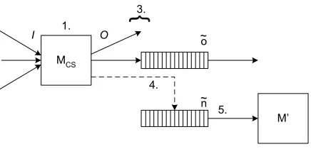
We start with an informal description. Machines switch sequentially, i.e., we have exactly one active machine M at any time. If this machine has clock out-ports, then besides its “normal” outputs, it can select the next message to be delivered by scheduling a buffer via one of these clock out-ports. If the selected message (i.e., a message at the selected position) exists in the buffer’s internal queue, it is delivered by the buffer and the unique receiving machine becomes the next active machine. If M tries to schedule multiple messages, only one is taken, and if it schedules none or the message does not exist, the default scheduler X (which exists since we consider a closed collection) becomes active.
Next we give a more precise, but still only semi-formal definition of runs. Runs and their probability spaces are defined inductively by the following algorithm for each tupleini of initial states of the machines of a closed collectionCˆ. The algorithm maintains variables for the states of all machines of the collection and treats each port as a variable over Σ∗, initialized with ǫ
except for clk⊳? := 1. The algorithm further maintains a variable MCS (“current scheduler”)
over machine names, initialized with MCS := X, for the name of the currently active simple
~
MCS
M’ O
I 1.
4.
5. 3.
n ~ o
Figure 4: Phases of the run algorithm.
1. Switch current scheduler: Switch the current machine MCS, i.e., set (s′, O) ← δMCS(s, I)
for its current state sand in-port valuesI. Then assign ǫto all in-ports of MCS.
2. Termination: If X is in a final state, the run stops. (As Xmade no outputs in this case, this only prevents repeated inputs at the default-clock in-port.)
3. Store outputs: For each simple out-porto! ofMCSwitho!6=ǫ, in their given order, switch
buffereowith inputo↔? :=o!. Then assign ǫto all these portso! and o↔?.
4. Clean up scheduling: If at least one clock out-port of MCS has a value6=ǫ, let n⊳! denote
the first such port according to their given order and assign ǫ to the others. Otherwise let clk⊳? := 1 andMCS:=Xand go to Phase 1.
5. Deliver scheduled message: Switchen with inputn⊳? :=n⊳!, setn? :=n↔! and then assign
ǫto all ports of en and ton⊳!. If n? =ǫ let clk⊳? := 1 andM
CS :=X. Else let MCS:= M′
for the unique machineM′ with n?∈ports(M′). Go to Phase 1.
Whenever a machine (this may be a buffer) with namenameM is switched from (s, I) to (s′, O),
we add a step (nameM, s, I, s′, O) to the run r with the following two restrictions. First, we
cut each input according to the respective length function, i.e., we replace I by I′ := I⌈lM(s).
Secondly, we do not add the step to the run ifI′ = (ǫ, . . . , ǫ), i.e., if nothing happens in reality. This gives a family of probability distributions (runCˆ,ini), one for each tupleini of initial states
of the machines of the collection. Moreover, for a set Mˆ of machines, we define the restriction of runs to those steps where a machine of Mˆ switches. This is called the view of Mˆ . Similar to runs, this gives a family of probability distributions (viewCˆ,ini(Mˆ )), one for each tupleini
of initial states.
Rigorous Definitions
We now define the probability space of runs rigorously. Since the semi-formal description is sufficient to understand our subsequent results and the rigorous definitions are quite technical, this subsection can be skipped at first reading.
Definition 3.15 (Global States of a Collection) Let ˆC be a complete, closed collection with de-fault schedulerX. LetPCˆ :={P | ∃M∈Cˆ :P ⊆out(PortsM)}where⊆denotes the subsequence
relation.
• The set of global states of ˆC is defined as
StatesCˆ :=×M∈CˆStatesM×Cˆ ×(Σ∗)ports(
ˆ C)× {
1, . . . ,5} × PCˆ ∪ {sfin}.
• The set of initial global statesof ˆC is defined as
IniCˆ :=×M∈CˆIniM× {X} × {f} × {1} × {()}
withf(clk⊳?) := 1and f(p) :=ǫ for p∈ports(Cˆ)\ {clk⊳?}.
3
On these global states, we define a global transition function. It reflects the informal run algorithm.
Definition 3.16 (Global Transition Function) Let ˆC be a complete, closed collection with de-fault scheduler X. We define the global transition function
δCˆ:StatesCˆ →Prob(StatesCˆ)
byδCˆ(sfin) :=sfin and otherwise by the following rules:
Phase 1: Switch current scheduler.
((sM)M∈Cˆ,MCS, f,1, P)→p ((s′M)M∈Cˆ,MCS, f
′,2,()) (1)
where, with I :=f(in(PortsMCS)) and O:=f
′(out(Ports
MCS)),
• p=Pr(δMCS(sMCS, I) = (s
′
MCS, O)),
• sM=s′M for allM∈Cˆ \ {MCS}, and
• f′(in(PortsMCS)) = (ǫ)
|in(PortsMCS)| and f ≡f′ on ports(Cˆ)\ports(MCS).
Phase 2: Termination.
((sM)M∈Cˆ,MCS, f,2, P)→sfin if sX ∈FinX; (2)
((sM)M∈Cˆ,MCS, f,2, P)→((sM)M∈Cˆ,MCS, f,3, P′) if sX 6∈FinX (3)
where P′ = (o!∈PortsMCS |o∈Σ
+∧f(o!)6=ǫ).
Phase 3: Store outputs.
((sM)M∈Cˆ,MCS, f,3,())→((sM)M∈Cˆ,MCS, f,4,()); (4)
((sM)M∈Cˆ,MCS, f,3, P)→((s′M)M∈Cˆ,MCS, f′,3, P′) ifP 6= () (5)
where there exists n∈Σ+ with
• (s′en,(ǫ)) =δne(sen,(ǫ, f(n!))),
• sM=s′M for allM∈Cˆ \ {en}, and
• f′(n!) =ǫ and f ≡f′ on ports(Cˆ)\ {n!}.
Phase 4: Clean up scheduling. Let Clks := (n⊳!∈Ports
MCS | f(n
⊳!)6=ǫ). Then
((sM)M∈Cˆ,MCS, f,4, P)→((sM)M∈Cˆ,X, f′,1,()) if Clks = () (6)
where f′(p) =ǫfor all p∈ports(Cˆ)\ {clk⊳?} and f′(clk⊳?) = 1, and
((sM)M∈Cˆ,MCS, f,4, P)→((sM)M∈Cˆ,MCS, f′,5, P′) if Clks 6= () (7)
where
• P′= (Clks[1]), and
• f′(Clks[1]c) =f(Clks[1]) and f′(p) =ǫ for allp∈ports(Cˆ)\ {Clks[1]c}.
Phase 5: Deliver scheduled message.
((sM)M∈Cˆ,MCS, f,5, P)→sfin if 6 ∃n∈Σ+:P = (n⊳!); (8)
((sM)M∈Cˆ,MCS, f,5,(n⊳!))→((s′M)M∈Cˆ,M
′
CS, f′,1,()) (9)
where there exists o∈Σ+ such that
• sM=s′M for allM∈Cˆ \ {en},
• (s′en,(o)) =δen(sen,(f(n⊳?), ǫ)),
and
• either o = ǫ and MCS′ = X and f′(clk⊳?) = 1 and f′(p) = ǫ for all p ∈ ports(Cˆ)\ {clk⊳?}
• or o6=ǫand n?∈PortsM′
CS and f
′(n?) =o andf′(p) =ǫfor all p∈ports(Cˆ)\ {n?}.
3
Rule (8) has only been included to define the function δ on the entire state space StatesCˆ as
claimed at the beginning of the definition. It will not matter in the execution since the previous state has to be in Phase 4, and this ensures that P contains exactly one clock port. Similarly, the other rules make no assumptions about reachable states. Furthermore, δ(s) is indeed an element of Prob(StatesCˆ) for everys∈StatesCˆ: It is deterministic for all states sexcept those
treated in Rule (1). For those, the claim follows immediately from the fact that δMCS(sMCS, I)
is a finite distribution.
Lemma 3.1 (Probabilities of State Sequences) Let ˆC be a complete, closed collection, and let an initial global state ini ∈IniCˆ be given. For each set of fixed-length sequences StatesiCˆ withi∈N, we can define a finite probability distribution PStatesCˆ,ini,i by
Pr(S) =
i
Y
j=2
Pr(δCˆ(Sj−1) =Sj)
for every sequence S= (S1, . . . , Si) over StatesCˆ withS1 =ini , and Pr(S) = 0 otherwise.
Furthermore, for every sequence S ∈ Statesi ˆ
C, let Rect(S) denote the corresponding
rect-angle of infinite sequences with this prefix, i.e., Rect(S) := {S′ ∈ States∞ˆ C | S
′⌈
i= S}. Then there exists a unique probability distribution PStatesCˆ,ini,∞ over States∞Cˆ whose value for every rectangle R:=Rect(S) withS ∈StatesiCˆ equals Pr(S), or more precisely,
PrPStatesCˆ,ini,∞(R) :=PrPStatesCˆ,ini,i(S).
We usually omit the indices “∞” and “i” of these distributions; this cannot lead to confusion.
2
Varyingini gives a family of probability distributions over States∞Cˆ; we write it
PStatesCˆ := (PStatesCˆ,ini)ini∈IniCˆ.
So far we have defined probabilities for sequences of entire global states. Each step in the runs introduced semi-formally above intuitively corresponds to the difference between two successive states: Moreover, only the switching of machines is considered in a run, i.e., the intermediate phases for termination checks and cleaning up scheduling are omitted, as well as the switching of machines with empty input (after application of the length function) because nothing happens then. We first define the set of possible steps, i.e., five-tuples containing the name of the currently switched machine M, its old state, its input tuple, its new state, and its output tuple. Furthermore, we define an encoding of steps as strings for the sole purpose of defining overall lengths of potential runs.
Definition 3.17 (Steps) The set of stepsis defined as
Steps := (Σ+◦ {∼, ǫ})×Σ∗×(Σ∗)∗×Σ∗×(Σ∗)∗.
Let ιSteps:Steps → Σ+ denote an efficient encoding from Steps into the non-empty strings over Σ. For all r = (ri)i∈I ∈Steps∗ let len(r) := Pi∈Isize(ιSteps(r)), and for r ∈ Steps∞ let
len(r) :=∞. 3
Definition 3.18 (Run Extraction) Let ˆC be a complete, closed collection. Then the run ex-traction of ˆC is the function
runCˆ:States∞Cˆ →Steps∗∪Steps∞
defined as follows. (It is independent of ˆC except for its domain.) Let S = (Si)i∈N ∈States∞ˆ
C where for eachi∈NeitherSi =sfin orSi= ((siM)M∈Cˆ,MiCS, fi, ji, Pi). Ifi∗ := min{i∈N|si = sfin} exists, let I := {1, . . . , i∗ −2}, otherwise I := N. We define a sequence pot step(S) =
((ni, si, Ii, s′i, Oi))i∈I as follows. (Thus we already omit the last termination check.)
• If Pi= () then, with M:=MiCS,
– ni :=nameM,
– si:=siM and s′i:=s i+1
M , and
– ifji= 1 then I
i :=fi(in(PortsM))⌈lM(si) andOi :=f
i+1(out(Ports
M)), elseIi:= (ǫ) and Oi := (ǫ).
• If Pi6= (), let p:=Pi[1] and p∈ports(en). Then
– ni :=n∼.
– si:=sien and s′i :=sien+1,
– Ii :=fi((n⊳?,n↔?)) and Oi :=fi+1((n↔!)).
Then runCˆ(S) := ((ni, si, Ii, s′i, Oi)∈pot step(S)|Ii6= (ǫ, . . . , ǫ)). For every number l∈N, let runCˆ,l denote the extraction of l-step prefixes of runs,
runCˆ,l:States∞Cˆ →
[
i≤l Stepsi
with runCˆ,l(S) :=runCˆ(S)⌈l. 3
The run extraction is a random variable on every probability space over States∞Cˆ. For our particular probability space, this induces a family runCˆ = (runCˆ,ini)ini∈IniCˆ of probability
distributions over Steps∗∪Steps∞ via
Prrunˆ
C,ini(r) :=PrPStatesCˆ,ini(run −1
ˆ C (r))
for all r ∈ Steps∗ ∪Steps∞, where run−ˆ1
C (r) is the set of pre-images of r. For a function l:IniCˆ →N, this similarly gives a family of probability distributions
runCˆ,l = (runCˆ,ini,l(ini))ini∈IniCˆ,
each over Si≤l(ini)Stepsi.