Use of Difference-Based Methods to Explore
Statistical and Mathematical Model
Discrepancy in Inverse Problems
H.T. Banks, Jared Catenacci and Shuhua Hu Center for Research in Scientific Computation
North Carolina State University Raleigh, NC 27695-8212 USA
September 15, 2015
Abstract
Normalized differences of several adjacent observations, referred to as pseudo mea-surement errors in this paper, are used in so-called difference-based estimation methods as building blocks for the variance estimate of measurement errors. Numerical results demonstrate that pseudo measurement errors can be used to serve the role of measure-ment errors. Based on this information, we propose the use of pseudo measuremeasure-ment errors to determine an appropriate statistical model and then to subsequently investi-gate whether there is a mathematical model misspecification or error. In the presence of model misspecification, we also propose to use the information provided by pseudo measurement errors to quantify uncertainty in parameter estimation by bootstrapping methods. A number of numerical examples are given to illustrate the effectiveness of these proposed methods.
Key Words: pseudo measurement errors, statistical model, inverse problems, model misspecification, bootstrapping.
1
Introduction
A number of difference-based methods have been proposed in the literature to estimate the variance of measurement errors in a nonparametric regression where the mean function of observations is unknown and estimated using some nonparametric methods (e.g., see [15, 19, 21, 22] and the reference therein). These methods involve differencing the data and do not require estimation of the mean function. Specifically, the estimated variance is defined as the weighted average of the squared normalized difference of ν+ 1 observations, where ν is an integer. These normalized differences of ν+ 1 observations are called pseudo measurement errors in this paper. The purpose of this paper is to illustrate how these pseudo measurement errors can be used as a possible way of detecting statistical model misspecification or discrepancy as well as mathematical model misspecification or discrepancy within the context of a least squares inverse problem. That is, given a set of observed data, a mathematical model describing the observed process is fitted to the data via a least squares formulation by estimating a set of unknown parameters. As has become conventional in inverse problems, we would also like to quantify the uncertainty present in the estimation of the mathematical model parameters using confidence intervals. To do this, one must have a correctly specified statistical model which describes the data collection process along with a mathematical model which is assumed to describe the process under observation. Typically, one uses residual plots as illustrated in [8, 12] to ensure that the assumptions made in specifying both the statistical and mathematical model are not violated. However, the residuals can only be computedafterthe inverse problem has been completed. Furthermore, if the residual plots do not illustrate the desired random patterns, it can be difficult, if not impossible to determine if this is caused by mathematical model discrepancy or statistical model discrepancy, or both. We will show how differencing techniques can be used directly on the data to deduce if the assumptions of the statistical model have been violated prior to running the inverse problem. Then residual plots can be used afterwards to verify that the mathematical model is sufficiently accurate.
We consider inverse or parameter estimation problems in the context of a parameterized (with vector parameter q ∈ Ωκq
⊂ Rκq) n-dimensional vector dynamical system (for a
physical or biological process) ormathematical model given by
dx
dt(t) = h(t,x(t),q), (1.1)
x(ts) = x0, (1.2)
with observation process
f(t;θ) =Cx(t;θ), (1.3)
where θ = (qT,x˜T
0)T ∈ Ω ⊂ Rκq+˜n = Rκθ,˜n ≤ n, κq is the number of unknown dynamic parameters, ˜n is the number of unknown initial conditions ˜x0, and the observation operator
C mapsRn toRm. The setsΩκq andΩare assumed known restraint sets for the parameters.
We make some standard assumptions (see [8, 12]) underlying our inverse problem formu-lations.
• Ωis a compact subset of Euclidian space ofRκθ andf(t;θ) is continuous on [0, T]×Ω.
Denote bθ as the estimated parameter for θ0 ∈Ω. The inverse problem is based on
sta-tistical assumptions on the observation error in the data. We consider a general statistical model of the form
Yj =f(tj;θ0) +g(tj;θ0,Ej), j = 1,2, . . . , N, (1.4)
where Yj = (Y1j, Y2j, . . . , Ymj)T, and f(tj;θ0) = (f1(tj;θ0), f2(tj;θ0), . . . , fm(tj;θ0))T
de-notes observations of the mathematical model describing the underlying physical or biological process with the nominal parametersθ0at the measurement pointtj. The so called
measure-ment or observation error attj is represented by g(tj;θ0,Ej) where Ej = (E1j,E2j, . . . ,Emj)T
is a m×1 random vector, and N is the total number of observations.
The simplest form of (1.4) is when g(tj;θ0,Ej) = Ej, this is known as an absolute
error model. Another popular choice for a statistical model is given by g(tj;θ0,Ej) =
f(tj;θ0)◦Ej which results in a relative error model, where ◦ denotes component-wise
multiplication of the vectors. In this work we will only concern ourselves with the special case of g(tj;θ0,Ej) =fγ(tj;θ0)◦Ej so that
Yj =f(tj;θ0) +fγ(tj;θ0)◦Ej, j = 1,2, . . . , N, (1.5)
where fγ(tj;θ0) = (fγ
1
1 (tj;θ0), fγ
2
2 (tj;θ0), . . . , fmγm(tj;θ0))T and γ = (γ1, γ2, . . . , γm). Here
fγ◦ denotes the component-wise exponentiation by γ of the vector function f followed by component-wise multiplication of the vectors fγ(tj;θ0) and Ej.
There are numerous examples in which such statistical models have been found appropri-ate if a proper value ofγ is chosen. These examples include modeling of HIV viral infections [5] for data consisting of CD4+ T cell counts with γ1 = 0 and viral RNA counts with
γ2 = 1.2; prion aggregation kinetic models [7] with γi = γ = 0.6; insect populations
under-going pesticide treatments [3, 4] with γ ≈.8 or .85; and cell proliferation studies modeling flow cytometry data with γ = 0.5 [8, p. 87], [24] for a dividing population of lymphocytes labeled with the intracellular dye CFSE. In this latter example, as cells divide, the highly fluorescent intracellular CFSE is partitioned evenly between two daughter cells. A flow cy-tometer measures the CFSE fluorescence intensity (FI) of labeled cells as a surrogate for the mass of CFSE within a cell, thus providing an indication of the number of times a cell has divided. In these applications we note that γ is a to-be-determined tuning parameter for the statistical model. Furthermore, we assume that for any fixed j, Eij, i= 1,2, . . . , m, are
independent with mean zero and Var(Eij) = σ02,i.
We remark that for the case where the measurement errors are heteroscedastic, the difference-based methods were specially designed for the general case (1.4). For these more general formulations the weights for the squared pseudo measurement errors (used in the estimation of the variance) involve kernel functions, and the bandwidth (a free parameter) of the kernel function has a strong influence on the resulting estimate. To our knowledge, a proper choice of bandwidth is still a current topic of research. In addition, variance estimation is not the focus of this paper.
To represent a collected data set, we let yj = (y1j, y2j, . . . , ymj)T be a realization ofYj,
where εj = (ε1j, ε2j, . . . , εmj)T is a realization of Ej, j = 1,2, . . . , N. We remark that
difference-based methods for calculation of pseudo measurement errors can also be used in the case where the components of Yj may be observed at different measurement points
(that is,Yij =fi(tij;θ0) +fγ
i
i (tij;θ0)Eij,j = 1,2, . . . , Ni,i= 1,2, . . . , m). But for notational
convenience, we only consider the case where all the components of Yj are observed at the
same measurement time points.
Of course, our modelf(tj;θ0) typically does not perfectly describe the underlying process
in question. This results in what we will refer to as mathematical model misspecification or discrepancy. Additionally, even in our assumption that the measurement errors can be described by (1.5), the value of γ is not known a priori. We will refer to this as statistical model misspecification or discrepancy.
For the sake of clarity, we present a basic example to make our motives clear. Consider a population under observation which is believed to follow the well known logistic model given by
˙
x(t) =bx(t)
1− x(t)
κ
, x(ts) =x0. (1.6)
Here x denotes the number of individuals, r is the intrinsic growth rate, and κ represents the carrying capacity and we assume that we can observe the number of individuals at times
tj, j = 1,2, , . . . , N. In this case we would have the statistical model
Yj =f(tj;θ0) +f(tj;θ)γEj, j = 1,2, . . . , N, (1.7)
where f(tj;θ) = x(tj;θ) denotes the solution to (1.6), (i.e. C = I), and θ = (b, κ, x0)T are
the unknown mathematical model parameters. Recall that if γ = 0 we have an absolute error model, which is interpreted as meaning that the observation errors are independent of the size of the population itself, and ifγ = 1 we have a relative error model, which indicates that the observation errors are a multiple of the population size itself. In general, for any
γ > 0 we are making the assumption that the observation errors are dependent on the size
of the population itself. Notice that E(Yj) =f(tj;θ0), and Var(Yj) =f(tj;θ0)2γσ02, thus the
variance is non-constant provided γ 6= 0.
In practice, one often assumes a specific statistical model (i.e., assumes a specific value for γi) and then chooses an appropriate method to carry out parameter estimation (for
example, if γi = 0, i = 1,2, . . . , m, then an ordinary least squares method is appropriate).
One can then use residual plots to determine whether or not the assumed statistical model is appropriate (e.g., see [8, Chapter 3]). If one assumes a statistical model with γi = 0,
i = 1,2, . . . , m, and the resulting residual plots exhibit a non random pattern, such as a
fan shaped pattern, then the assumed statistical model is not reasonable. In the case where the assumed statistical model is inappropriate, one tries another set of values for γi’s and
carries out another inverse problem. This may be done iteratively until one finds values ˆγi’s
such that the plot of the modified residuals rij/|yij−fi(tj; ˆθ)|bγi versustj forms a horizontal
band around the horizontal axis (where rij = yij −fi(tj;bθ) is the residual and bθ denotes
paper, we propose to use the information provided by the pseudo measurement errors to directly determine appropriate values for the γi’s. We note that difference-based methods
used to calculate pseudo measurement errorsdo not involve any inverse problem calculations
and are independent of the chosen mathematical model. Hence, if our proposed method is successful, it should provide a much more efficient and accurate way to determine appropriate values for theγi’s.
After determining appropriate values for the γi’s (i.e., an appropriate statistical model),
one may then use pseudo measurement errors to determine whether there is a mathematical model error. Specifically, one first uses the appropriate statistical model (chosen based on the information provided by pseudo measurement errors) to carry out parameter estimation. Then one compares the residual plot and the plot of ˆεij versustj to determine whether there
is a mathematical model misspecification. For example, if there is a discernible divergence between these two plots, then there is a mathematical model error and the degree of this error is determined by the degree of the divergence. Specifically, the difference between residuals and ˆεij’s provides some prior information on this error. However, we remark that no
discernible divergence between these two plots does not implythat there is no mathematical model error. As we shall see, there are some cases where two different mathematical models could give the same solution in the given sampling time region.
In the presence of mathematical model misspecification, we also propose to use the in-formation provided by pseudo measurement errors to preform bootstrapping to quantify the uncertainty in parameter estimates. Bootstrapping is a popular tool for construction of confidence intervals for parameter estimators (e.g., see [8, Chapter 3] and [17]). It involves constructing a family of samples or simulated data sets based on random sampling with replacement. One uses each of these samples to solve the inverse problem to obtain a new estimate, and then constructs the confidence intervals based on this family of estimates for the parameter estimators. We remark that there are two common ways to construct a family of samples or simulated data sets. One involves resampling the original data set, and it is based on the assumption that the original data are independent and identically distributed (i.i.d.). However, this method does not work well for cases where models are used to describe dynamic systems as observations are often not identically distributed even in the case where measurement errors are independent and identically distributed. The other method involves resampling residuals from an initial estimation to the original data set, and this is based on the assumptions that the regression function correctly specifies the observed part of the system and the first two moments of measurement errors are correctly specified (that is, the given statistical model is correctly specified). We thus see that this method does not work for the case where there is a mathematical modeling misspecification, which is often the situation in describing a real system. To alleviate this difficulty, we propose to use difference-based methods to obtain the pseudo measurement errors and then create bootstrapping samples using random sampling with replacement from these pseudo measurement errors.
illustrate how to carry out bootstrapping to quantify the uncertainty of corresponding param-eter estimators in the presence of model misspecification. Finally, in Section 5 we conclude the paper with some summary remarks and future research efforts.
2
Difference-Based Methods
All of the difference-based methods are based on the assumption that the true or nominal regression function f is sufficiently smooth and the maximum of the length of sampling time intervals (i.e., max{tj+1−tj, j = 1,2, . . . , N−1}) is sufficiently small. The estimated variance
is defined as the weighted average of the squared normalized differences ofν+1 observations. Specifically, the normalized differences ofν+ 1 observations,pseudo measurement errors, are defined as being either symmetric around yij as in
ˆ
εij = ν
X
k=0
wkyi,j−hν+1 2
i
+k+1, j =
ν
2
,ν
2
+ 1, . . . , N −ν
2
, i= 1,2, . . . , m, (2.1)
or asymmetric about yij as in
ˆ
εij = ν
X
k=0
wkyi,j+k, j = 1,2, . . . , N −ν, i= 1,2, . . . , m. (2.2)
Here [a] denotes the smallest integer that is greater than or equal to a, and the wk’s are
some real numbers which satisfy the conditions
ν
X
k=0
wk = 0,
ν
X
k=0
w2k= 1.
We remark that the above conditions are necessary to obtain an asymptotically unbiased estimator for the variance (e.g., see [21]) and so that the choice of the form for the pseudo measurement errors (i.e., choosing either (2.1) or (2.2)) does not affect the asymptotic result (e.g., see [19]).
Based on the choice for the values of ν and wk’s, we introduce here three of these
difference-based methods. One of them involves first-order backward differencing data (i.e.,
ν = 1) and the associated pseudo measurement errors are calculated as follows:
ˆ
ε1st
ij =
1
√
2(yi,j−1−yi,j), j = 2,3, . . . , N, i= 1,2, . . . , m. (2.3)
For the case γi = 0 (i.e., constant variance error), the estimate for σ0,i is then given by
ˆ
σ1st
0,i =
v u u
t 1
N −1
N
X
j=2
ˆ
ε1st
ij
2
, i= 1,2, . . . , m. (2.4)
Another method involves second-order differencing data; that is ν = 2. The pseudo mea-surement errors are given by
ˆ
ε2nd
ij =
1
√
For the case γi = 0, the associated estimate for σ0,i is then given by
ˆ
σ2nd
0,i =
v u u
t 1
N−2
NX−1
j=2
ˆ
ε2nd
ij
2
, i= 1,2, . . . , m. (2.6)
The last method we consider involves applying a first-order differencing operatorl times (i.e. a lth order difference), where l is some integer. Let ∆l denote the first order differencing operator applied l times with ∆yij =yi,j+1−yij, j = 1,2, . . . , N −1, i= 1,2, . . . , m. Then
pseudo measurement errors are calculated as follows:
ˆ
ε1st-l
ij =
s
2l l
−1
∆ly
j, j = 1,2,3, . . . , N −l, i= 1,2, . . . , m, (2.7)
where
2l l
= (2l)!
(l!)2 with l! be the factorial of l. For the case γi = 0, the estimate forσ0,i
is then given by
ˆ
σ1st-l
0,i =
v u u
t 1
N −l
N−l
X
j=1
(ˆε1st-l
ij )2, i= 1,2, . . . , m. (2.8)
It was suggested in [23] that the choice ofl = 3 works well in practice. This is also the value that we use for l in all the numerical results shown in this paper.
We remark that for the case where one suspects that observation coordinates ofYj may
have different constant variance (i.e., σ0,i may not be equal to σ0,k), one usually uses an
iterative process to carry out parameter estimation for mathematical model parameters and
σ0,i’s (e.g., see [8, Section 3.2.2] for details). However, by using the above methods one is
able to obtain the estimates for σ0,i’s and hence one does not need to use such an iterative
inverse problem procedure. This can significantly speed up the desired inverse problem methodology.
3
Application on Determining an Appropriate
Statis-tical Model to Use
In this section, we first apply the three methods introduced in Section 2 to some simulated data sets to demostrate the accuracy of these methods as well as the accuracy of the proposed method in using the information provided by pseudo measurement errors to determine an appropriate statistical model. We then apply these methods to some experimental data sets to determine the appropriate statistical models.
3.1
Numerical Results for Simulated Data Sets
3.1.1 Example 1: Logistic Growth Model
We consider the standard logistic growth model
˙
x=bx1− x
κ
, x(ts) =x0 (3.1)
as described in Section 1.
We assume that we can observe the number of individuals; that is, f =x. To generate the simulated data, we simulate (3.1) with parameter values and initial values chosen as
b = 3, κ = 100, x0 = 10. We then impose a normal distribution on Ej with zero mean and
standard deviationσ0 = 0.05, where the measurement time points aretj =ts+ (j−1)
tf −ts
N −1
with ts = 0, tf = 2.5, j = 1,2, . . . , N and N = 201. In other words, the simulated data set
{yj}Nj=1 is generated as follows:
yj =x(tj) +xγ(tj)εj, j = 1,2, . . . , N, (3.2)
where εj is a relization of Ej. We first will confirm that the pseudo measurement errors
provide a reasonable approximation of the true measurement errors εj. Then we show that
the pseudo measurement errors can be used to determine the unknown value of γ.
Table 1 summarizes the estimates for σ0 found using the three methods introduced in
Section 2 for the case where γ = 0 in (3.2). From this table, we see that the last two methods give reasonable estimates for σ0 while the first method considerably overestimates
the value of σ0. But we do see from other numerical results (see the SIR example discussed
in the next section) that this simple method does give a good estimate for some examples. But in summary, this suggests that this first-order differencing method does not consistently perform well. This is consistent with the observation made in [15], wherein it is suggested that the first-order differencing method should not be used since it does not always behave well.
σ0 σˆ
1st
0 σˆ
2nd
0 σˆ
1st-3
0
5.000e-02 3.930e-01 5.210e-02 5.216e-02
Table 1: Results for the logistic example in the case where γ = 0: the true value of σ0 as
well as its estimates obtained using the three mentioned methods (ˆσ1st
0 is obtained using the
first-order differencing method, ˆσ2nd
0 is obtained using the second-order differencing method,
and ˆσ1st-3
0 is obtained by applying the first-order differencing operator for 3 times).
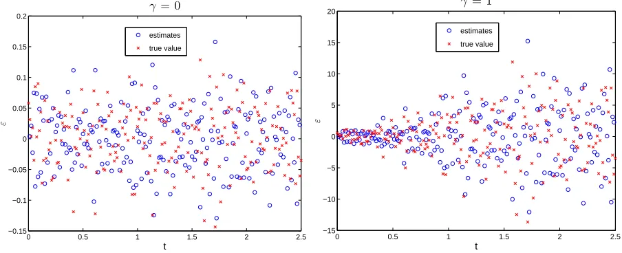
Figure 1 presents the plot of pseudo measurement errors ˆε1st
j (obtained using the
first-order differencing method and denoted as “estimates” in the legend of this figure) versus tj
and the plot ofεj (simulated measurement errors and denoted as “true values” in the legend)
versus tj for the cases where γ = 0 (left column) and γ = 1 (right column) in (3.2). From
this figure, we see that for the case where γ = 0 the plot of ˆε1st
j versus tj diverges from the
plot of εj versus tj except at the very end. This is consistent with considerable difference
of the estimate ˆσ1st
0 from its true value. However, for the case where γ = 1 the time plot
0 0.5 1 1.5 2 2.5 −0.8
−0.7 −0.6 −0.5 −0.4 −0.3 −0.2 −0.1 0 0.1 0.2
γ = 0
t
ε
estimates true value
0 0.5 1 1.5 2 2.5
−20 −15 −10 −5 0 5 10 15
t
ε
γ= 1
estimates true value
Figure 1: Comparison of the plot of ˆε1st
j (denoted as “estimates” in the legend) versus tj
and the plot of εj (denoted as “true value”) versus tj : (left panel) results obtained for
γ = 0; (right panel) results obtained for γ = 1, where ˆε1st
j ’s are obtained by the first-order
differencing method.
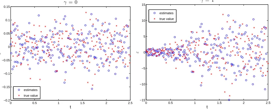
This suggests that for this case this method works well. Figure 2 illustrates the results for the pseudo measurement errors ˆε2nd
j obtained using second-order differencing method while
Figure 3 depicts the results for the pseudo measurement errors ˆε1st-3
j obtained by applying the
first-ordering differencing operator for 3 times. From these two figures, we see that the time
0 0.5 1 1.5 2 2.5
−0.15 −0.1 −0.05 0 0.05 0.1 0.15 0.2
γ= 0
t
ε
estimates
true value
0 0.5 1 1.5 2 2.5
−15 −10 −5 0 5 10 15 20
t
ε
γ= 1
estimates true value
Figure 2: Comparison of the plot of the ˆε2nd
j (denoted as “estimates” in the legend) versus
tj and the plot of εj (denoted as “true value”) versus tj for the case γ = 0 (left panel) and
the case γ = 1 (right panel), where the ˆε2nd
j are obtained using the second-order differencing
method.
0 0.5 1 1.5 2 2.5 −0.2
−0.15 −0.1 −0.05 0 0.05 0.1 0.15
γ= 0
t
ε
estimates
true value
0 0.5 1 1.5 2 2.5
−15 −10 −5 0 5 10 15
t
ε
γ= 1
estimates true value
Figure 3: Comparison of the plot of the ˆε1st-3
j (denoted as “estimates” in the legend) versustj
and the plot of εj (denoted as “true value”) versus tj for the case γ = 0 (left panel) and the
case γ= 1 (right panel), where the ˆε1st-3
j are obtained by applying the first-order differencing
operator for 3 times.
errors for both the constant variance error case and the relative error case.
Of course, in practice one does not have a value of the measurement errors themselves, rather only the data measurement {yj}Nj=1 is known. We claim that if the pseudo
measure-ment errors provide a reasonable approximation of the true (but unknown) measuremeasure-ment errors, then we can use the pseudo measurement errors to determine an appropriate value for γ. For example, if the plot of pseudo measurement errors ˆεj versus tj seems to form a
horizontal band around the horizontal axis, thenγ = 0 may be appropriate. However, if one finds that the plot of ˆεj versus tj does not appear to be identically distributed, then γ 6= 0
and one needs to find a proper nonzero value for γ. To do this, we try different values for γ
until one finds a value ˆγ such that the plot of ˆεj/|yj−εˆj|γˆ versustj forms a horizontal band
around the horizontal axis. To verify whether or not this works, we take this logistic model with simulated data generated using γ = 1 as an example. We note that for this data set the plot of ˆεj versus tj (e.g., see the right panel of Figure 3) exhibits a fan shaped pattern.
To begin with, we choose ˜γ = 2. The resulting plot forηj˜γ= ˆε1st-3
j /|yj−εˆ
1st-3
j |
˜
γ versust j with
˜
γ = 2 is shown in the left panel of Figure 4, where the ˆε1st-3
j are obtained by applying the
first-order differencing operator three times. We observe from this plot that it has an inverted fan shaped pattern. This indicates that a proper value for γ is between 0 and 2. We then plotted ηjγ˜ versus tj with ˜γ = 1 (shown in the right panel of Figure 4) and found that they
0 0.5 1 1.5 2 2.5 −8
−6 −4 −2 0 2 4 6 8 10x 10
−3
t
η
0 0.5 1 1.5 2 2.5
−0.15 −0.1 −0.05 0 0.05 0.1 0.15 0.2
t
η
Figure 4: Plot ofηj˜γ = ˆε1st-3
j /|yj−εˆ
1st-3
j |˜
γ versust
j for the case where the simulated data were
generated with γ = 1: (left panel) ˜γ = 2; (right panel) ˜γ = 1.
0 0.5 1 1.5 2 2.5
−6 −4 −2 0 2 4 6 8x 10
−3
t
η
0 0.5 1 1.5 2 2.5
−0.15 −0.1 −0.05 0 0.05 0.1 0.15 0.2 0.25
t
η
Figure 5: Plot of ηj˜γ = ˆε
2nd
j /|yj −εˆ
2nd
j |˜ γ
versus tj for the case where the simulated data were
generated with γ = 1: (left panel) ˜γ = 2; (right panel) ˜γ = 1.
3.1.2 Example 2: SIR Model
We next consider a simple SIR model described by the following system of ordinary differ-ential equations
˙
S=−βSI,
˙
I =βSI−δI,
˙
R=δI,
(S(ts), I(ts), R(ts)) = (S0, I0, R0).
(3.3)
Here S, I and R respectively denote the ratios of the numbers of susceptible, infected, and recovered individuals to the total number of individuals (so they are dimensionless), β
denotes the infection rate, andδ is the recover rate.
For demonstration purpose, we assume that we can observe all these three states; that
is, f = (S, I, R)T. For all the results shown below, the parameter values and initial values
are chosen asβ = 6, δ = 3, S0 = 0.7, I0 = 0.2, R0 = 0.1. To generate the simulated data, we
impose a normal distribution on E1j with zero mean and standard deviation σ0,1 = 0.01, a
normal distribution onE2j with zero mean andσ0,2 = 0.005 and a normal distribution onE3j
with zero mean andσ0,3 = 0.02, where the measurement time points aretj =ts+(j−1)
tf −ts
N −1
with ts = 0, tf = 2 andN = 201, j = 1,2, . . . , N.
Table 2 summarizes the estimates for σ0,i by using the three methods introduced in
Section 2 for the case where γi = 0, i = 1,2,3. From this table, we see that all three
methods give reasonable estimates for σ0,i.
σ0,i 1.000e-02 5.000e-03 2.000e-02
ˆ
σ1st
0,i 1.074e-02 5.295e-03 2.049e-02
ˆ
σ2nd
0,i 1.039e-02 5.297e-03 2.009e-02
ˆ
σ1st-3
0,i 1.043e-02 5.368e-03 1.996e-02
Table 2: Results for the SIR example in the case where γi = 0, i = 1,2,3: the value of σ0,i
as well as its estimates obtained using the three methods introduced in Section 2.
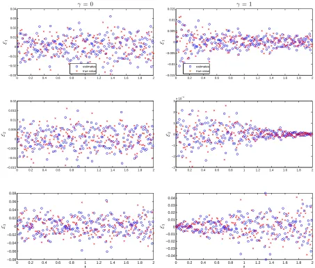
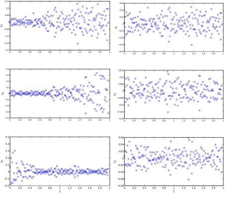
Figure 6 presents the plots of pseudo measurement errors ˆε1st
ij (obtained using first-order
differencing method and denoted as “estimates” in the legend of this figure) versus tj and
the plot of εij (simulated measurement errors and denoted as “true value” in the legend of
this figure) versustj for the cases whereγ1 =γ2 =γ3 = 0 (left column) andγ1 =γ2 =γ3 = 1
(right column). From this figure, we see that for the case γ1 =γ2 =γ3 = 0 the time plot for
ˆ
ε1st
i· exhibits exactly the same pattern as that forεi·. However, for the case γ1 =γ2 =γ3 = 1,
there is a discernible divergence between the plot of ˆε1st
2j versus tj and the plot of ε2j versus
tj. This again demonstrates that the first-order differencing method does not consistently
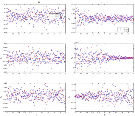
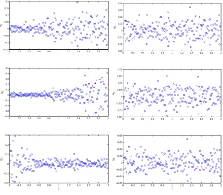
perform well. Figure 7 illustrates the results for the pseudo measurement errors ˆε2nd
ij obtained
using the second-order differencing method while Figure 8 depicts the results for the pseudo measurement errors ˆε1st-3
ij obtained by applying the first-order differencing operator 3 times.
0 0.2 0.4 0.6 0.8 1 1.2 1.4 1.6 1.8 2 −0.04
−0.03 −0.02 −0.01 0 0.01 0.02 0.03 0.04
γ= 0
E1
estimates true value
0 0.2 0.4 0.6 0.8 1 1.2 1.4 1.6 1.8 2 −0.015
−0.01 −0.005 0 0.005 0.01 0.015 0.02
E2
0 0.2 0.4 0.6 0.8 1 1.2 1.4 1.6 1.8 2
−0.08 −0.06 −0.04 −0.02 0 0.02 0.04 0.06
E3
t
0 0.2 0.4 0.6 0.8 1 1.2 1.4 1.6 1.8 2 −0.015
−0.01 −0.005 0 0.005 0.01 0.015 0.02
γ= 1
E1
estimates true value
0 0.2 0.4 0.6 0.8 1 1.2 1.4 1.6 1.8 2 −4
−3 −2 −1 0 1 2 3 4x 10
−3
E2
0 0.2 0.4 0.6 0.8 1 1.2 1.4 1.6 1.8 2
−0.04 −0.02 0 0.02 0.04
E3
t
Figure 6: Comparison of the plot of ˆε1st
ij (denoted as “estimates” in the legend) versus tj and
the plot ofεij (denoted as “true value”) versus tj for the caseγ1 =γ2 =γ3 = 0 (left column)
and the case γ1 =γ2 =γ3 = 1 (right column).
0 0.2 0.4 0.6 0.8 1 1.2 1.4 1.6 1.8 2 −0.03
−0.02 −0.01 0 0.01 0.02 0.03 0.04
γ= 0
E1
estimates true value
0 0.2 0.4 0.6 0.8 1 1.2 1.4 1.6 1.8 2 −0.015
−0.01 −0.005 0 0.005 0.01 0.015 0.02
E2
0 0.2 0.4 0.6 0.8 1 1.2 1.4 1.6 1.8 2
−0.08 −0.06 −0.04 −0.02 0 0.02 0.04 0.06 0.08
E3
t
0 0.2 0.4 0.6 0.8 1 1.2 1.4 1.6 1.8 2 −0.015
−0.01 −0.005 0 0.005 0.01 0.015
γ= 1
E1
estimates true value
0 0.2 0.4 0.6 0.8 1 1.2 1.4 1.6 1.8 2 −3
−2 −1 0 1 2 3x 10
−3
E2
0 0.2 0.4 0.6 0.8 1 1.2 1.4 1.6 1.8 2
−0.04 −0.03 −0.02 −0.01 0 0.01 0.02 0.03 0.04
E3
t
Figure 7: Comparison of the plot of ˆε2nd
ij (denoted as “estimates” in the legend) versus tj
and the plot of εij (denoted as “true value”) versus tj for the case γ1 = γ2 = γ3 = 0 (left
0 0.2 0.4 0.6 0.8 1 1.2 1.4 1.6 1.8 2 −0.04
−0.03 −0.02 −0.01 0 0.01 0.02 0.03
γ= 0
E1
estimates true value
0 0.2 0.4 0.6 0.8 1 1.2 1.4 1.6 1.8 2 −0.02
−0.015 −0.01 −0.005 0 0.005 0.01 0.015 0.02
E2
0 0.2 0.4 0.6 0.8 1 1.2 1.4 1.6 1.8 2
−0.08 −0.06 −0.04 −0.02 0 0.02 0.04 0.06
E3
t
0 0.2 0.4 0.6 0.8 1 1.2 1.4 1.6 1.8 2 −0.015
−0.01 −0.005 0 0.005 0.01 0.015
γ= 1
E1
estimates true value
0 0.2 0.4 0.6 0.8 1 1.2 1.4 1.6 1.8 2 −3
−2 −1 0 1 2 3x 10
−3
E2
0 0.2 0.4 0.6 0.8 1 1.2 1.4 1.6 1.8 2
−0.04 −0.02 0 0.02 0.04
E3
t
Figure 8: Comparison of the plot of ˆε1st-3
ij (denoted as “estimates” in the legend) versus tj
and the plot of εij (denoted as “true value”) versus tj for the case γ1 = γ2 = γ3 = 0 (left
The above numerical results again reveal that if difference-based methods work, then the obtained pseudo measurement errors can be used to play the role as measurement errors and hence can be used to determine appropriate values forγi’s. Here we take this SIR model with
simulated data generated using γ1 =γ2 = γ3 = 1 as another example to further verify the
method used in Section 3.1.1 for determining appropriate values forγi’s in the case where the
pseudo measurement errors do not appear to be identically distributed. Specifically, we try different values forγi until one finds a value ˆγi such that the plot of ˆεij/|yij−εˆij|γˆi versustj
forms a horizontal band around the horizontal axis. We note that for this data set both the plot of ˆε1j versustj and the plot of ˆε2j versustj (e.g., see the right column of Figure 8) exhibit
a fan shaped pattern while the plot of ˆε3j versus tj exhibits an inverted fan shaped pattern.
For a start, we choose ˜γi = 2, i = 1,2,3. The resulting plots for η˜γ
i
ij = ˆε
1st-3
ij /|yij −εˆ
1st-3
ij |˜γ
i
versus tj with ˜γi = 2 and i = 1,2,3, are shown in the left column of Figure 9, where
the ˆε1st-3
ij are obtained by applying the first-order differencing operator for three times. We
observe from these plots that the patterns for all these three plots are inverted (i.e., the plot previously having a fan shaped pattern now has an inverted fan shaped pattern, and the plot previously having an inverted fan shaped pattern now have a fan shaped pattern). This indicates that a proper value forγi is between 0 and 2, i= 1,2,3. We then plotted η˜γ
i
ij
versustj with ˜γ1 = ˜γ2 = ˜γ3 = 1 (shown in the right column of Figure 9) and found that they
all appear to be identically distributed. Figure 10 depicts the results using the second-order differencing method. We observe similar patterns. These results again demonstrate that our proposed method of using pseudo measurement errors to determine an appropriate value for
0 0.2 0.4 0.6 0.8 1 1.2 1.4 1.6 1.8 2 −0.2
−0.15 −0.1 −0.05 0 0.05 0.1 0.15
η1
0 0.2 0.4 0.6 0.8 1 1.2 1.4 1.6 1.8 2 −0.4
−0.3 −0.2 −0.1 0 0.1 0.2 0.3 0.4
η2
0 0.2 0.4 0.6 0.8 1 1.2 1.4 1.6 1.8 2 −0.2
−0.1 0 0.1 0.2 0.3 0.4 0.5
η3
t
0 0.2 0.4 0.6 0.8 1 1.2 1.4 1.6 1.8 2 −0.04
−0.03 −0.02 −0.01 0 0.01 0.02 0.03
η1
0 0.2 0.4 0.6 0.8 1 1.2 1.4 1.6 1.8 2 −0.02
−0.015 −0.01 −0.005 0 0.005 0.01 0.015
η2
0 0.2 0.4 0.6 0.8 1 1.2 1.4 1.6 1.8 2 −0.08
−0.06 −0.04 −0.02 0 0.02 0.04 0.06
η3
t
Figure 9: Plot of ηγ˜i
ij = ˆε
1st-3
ij /|yij −εˆ
1st-3
ij |˜ γi
versus tj for the case where the simulated data
were generated with γ1 = γ2 = γ3 = 1: (left panel) ˜γ1 = ˜γ2 = ˜γ3 = 2; (right panel)
˜
0 0.2 0.4 0.6 0.8 1 1.2 1.4 1.6 1.8 2 −0.15
−0.1 −0.05 0 0.05 0.1 0.15 0.2
η
1
0 0.2 0.4 0.6 0.8 1 1.2 1.4 1.6 1.8 2 −0.4
−0.3 −0.2 −0.1 0 0.1 0.2 0.3 0.4 0.5
η2
0 0.2 0.4 0.6 0.8 1 1.2 1.4 1.6 1.8 2 −0.2
−0.1 0 0.1 0.2 0.3
η
3
t
0 0.2 0.4 0.6 0.8 1 1.2 1.4 1.6 1.8 2 −0.03
−0.02 −0.01 0 0.01 0.02 0.03 0.04
η
1
0 0.2 0.4 0.6 0.8 1 1.2 1.4 1.6 1.8 2 −0.015
−0.01 −0.005 0 0.005 0.01 0.015 0.02
η2
0 0.2 0.4 0.6 0.8 1 1.2 1.4 1.6 1.8 2 −0.06
−0.04 −0.02 0 0.02 0.04 0.06 0.08
η
3
t
Figure 10: Plot of η˜γi
ij = ˆε
2nd
ij /|yij −εˆ
2nd
ij |γ˜
i
versus tj for the case where the simulated data
were generated with γ1 = γ2 = γ3 = 1: (left panel) ˜γ1 = ˜γ2 = ˜γ3 = 2; (right panel)
˜
3.2
Numerical Results for Experimental Data Sets
In this section, we apply the difference-based methods to some experimental data sets to determine an appropriate value for γ. Since the first-order differencing method does not consistently perform well, we only use the second-order differencing method and the method for applying the first-order differencing operator 3 times for these data sets.
3.2.1 Daphnia magna Data Set
Here we consider the survival data collected for Daphnia magna that were presented in [1]. Specifically, ninety daphnids (neonates) were longitudinally observed and survival was recorded daily, and an ordinary least squares method was used in this paper to estimate the mortality rate.
Figure 11 presents the time plot results for the pseudo measurement errors obtained using the second-order differencing method (left) and the method for applying the first-order differencing operator three times (right). We observe from the right plot of this figure that pseudo measurement errors form a horizontal band around the line ε= 0. The similar pattern can be observed from the left plot of Figure 11 except several outliers. This indicates that the absolute error model (i.e.,γ = 0) may be correct for this case. This provides support for using ordinary least squares method for parameter estimation in [1].
0 10 20 30 40 50 60 70 80 90
−1.5 −1 −0.5 0 0.5 1 1.5 2 2.5
t
ε
0 10 20 30 40 50 60 70 80 90
−1.5 −1 −0.5 0 0.5 1 1.5
t
ε
Figure 11: Time plots for pseudo measurement errors obtained for the Daphnia data set presented in [1]: (left panel) using the second-order differencing method; (right panel) using the method for applying the first-order differencing operator for three times (right).
3.2.2 CFSE Data Set
Here we consider the flow cytometry data presented in [8, Section 3.5.3] for a dividing population of lymphocytes labeled with the intracellular dye CFSE. The observable is the number of cells measured at time sk with log-fluorescence intensity in the region [zi, zi+1),
we re-index the data collection points {(sk, zi)} by {tj}; that is, the elements in the set
{tj}513j=513(k k−1)+1 correspond to the elements in the set {(sk, zi)}513i=1 , k = 1,2, . . . ,7.
Figure 12 depicts results obtained using the second-order diferencing method. Specif-ically, the left panel shows the plot of pseudo measurement errors ˆε2nd
j versus j, and the
right panel illustrates the plot of ηj˜γ = ˆε2nd
j /|yj −εˆ
2nd
j |
˜
γ versus j with ˜γ = 0.5, where the
vertical lines delineate the pseudo measurement errors obtained in time intervals [sk, sk+1),
k = 1,2, . . . ,7. We observe from the left panel of Figure 12 that pseudo measurement errors
500 1000 1500 2000 2500 3000 3500
−5000 −4000 −3000 −2000 −1000 0 1000 2000 3000 4000 5000
˜
γ= 0
ε
500 1000 1500 2000 2500 3000 3500 −50
0 50 100 150 200
˜
γ= 0.5
ε
Figure 12: Plots for pseudo measurement errors obtained for the CFSE data set presented in [8, Section 3.5.3] by using the second-order differencing method: (left panel) plot of ˆεj
versus j; (right panel) plot ofηj˜γ = ˆε2nd
j /|yj −εˆ
2nd
j |
˜
γ versus j with ˜γ = 0.5. The vertical lines
delineate the pseudo measurement errors obtained in time intervals [sk, sk+1),k = 1,2, . . . ,7.
are far from identically distributed. This is also true even in each subinterval [sk, sk+1).
Hence, γ = 0 is not a reasonable choice for this data set. This conclusion is consistent with the one made in [8, Section 3.5.3] where residual plots were used to determine an appropriate value for γ. Results in the right panel of Figure 12 imply that in each subinterval [sk, sk+1)
theηjγ˜’s appear to be identically distributed except some outliers. This indicates thatγ = 0.5 may be appropriate in each of these subintervals. We also observe from this plot that the bandwidth formed by the plot ofηj˜γ’s in the last two subintervals are larger than the ones for those subintervals located in the middle, which suggests that we may have different constant variance for ηγj˜ in these subintervals. This is inconsistent with the conclusion made in [8,
Section 3.5.3] where residual plots reveal that the modified residuals rj/|yj−f(tj; ˆθ)|γ˜ with
˜
γ = 0.5 appear to be identically distributed in the whole interval. Figure 13 demonstrates the results obtained by applying the first-order differencing operator three times. We observe similar patterns as that obtained by the second-order differencing method. As we discussed earlier in the Introduction, this inconsistency suggests that there may be a mathematical model misspecification involved.
here. The Bocharov, et al., investigations raised the question of whether cell proliferation models which allowed for asymmetric label division might be better suited to describe our human cell proliferation data. In [10] we revisited these data sets for the possibility of math-ematical model misspecification. In these investigations we used statistically based model comparison tests and found seemingly contradictory results. In one third of the data sets studied, we found support for the hypothesis that mathematical models permitting asym-metric label division did not improve the fits-to-data. However, for two thirds of the data sets, it was found that allowing asymmetric division does appear to lead to statistically sig-nificantly better agreement with the data. While there may be other confounding factors, the findings of [10] support the suggestion that there may be mathematical modeling error in the earlier CSFE labeled cell proliferation studies of [8, 9, 11, 18]. Thus the findings in the present analysis are consistent with notion of a mathematical modeling misspecification in the earlier findings reported in [10].
500 1000 1500 2000 2500 3000 3500
−5000 −4000 −3000 −2000 −1000 0 1000 2000 3000 4000 5000
˜
γ= 0
ε
500 1000 1500 2000 2500 3000 3500 −50
0 50 100 150 200 250 300 350
˜
γ= 0.5
ε
Figure 13: Plots for pseudo measurement errors obtained for the CFSE data set presented in [8, Section 3.5.3] by applying the first-order differencing operators for three times: (left panel) plot of ˆεj versus j; (right panel) plot of ηj˜γ = ˆε
1st-3
j /|yj −εˆ
1st-3
j |˜γ versus j with ˜γ = 0.5. The
vertical lines delineate the pseudo measurement errors obtained in time intervals [sk, sk+1),
k = 1,2, . . . ,7.
4
Bootstrapping in the Presence of Mathematical Model
Misspecification
For demonstration purpose, we use the simulated data set that was generated by the logistic growth model (3.1) using an absolute error model (γ = 0). Specifically, the data set
{yj}is generated as follows: we first simulate (3.1) with model parameters and initial values
given by b = 0.8, κ = 200, x0 = 10; we then impose a normal distribution on Ej with zero
mean and standard deviation σ0 = 0.2 to generate a realization εj of measure error Ej (i.e.,
constant variance error), where again the measurement time points aretj =ts+(j−1)
tf −ts
N −1
with ts = 0, tf = 2 and j = 1,2, . . . , N, with N = 201. We finally add this noise to the
simulated model solution (that is, yj = x(tj) + εj with x(t) the solution to the logistic
model (3.1)). The resulting data are illustrated in Figure 14.
0 0.2 0.4 0.6 0.8 1 1.2 1.4 1.6 1.8 2 10
15 20 25 30 35 40 45
t
x
data model sol
Figure 14: Results for fitting exponential growth model (4.1) to the simulated data generated by the logistic growth model (3.1).
In practice, one has no idea how {yj} is generated. Based on the information provided
by the plot of this data set, one may choose to use an exponential growth model to describe the data, i.e.,
˙˜
x=bx,˜ x˜(ts) =x0, (4.1)
where the parameter b needs to be estimated from the data. Hence, the data is assumed to be generated by
Yj =f(tj;b0) +Ej, j = 1,2, . . . , N, (4.2)
where f(t;b) = ˜x(t;b) = x0exp(bt). In practice, one may have no knowledge of the
mea-surement errors either. Since both second-order differencing method and the method for applying the first-order differencing operator 3 times work well, here we just use the second-order differencing method to determine a proper statistical model. The resulting plot for the pseudo measurement errors ˆεj versus tj is illustrated in the left panel of Figure 15. From
least squares method to do parameter estimation.
ˆb= arg min
b∈[b,¯b]
N
X
j=1
(yj −f(tj;b))2, (4.3)
where b and ¯b are some constants. The resulting model fit is illustrated in Figure 14. From this figure, we see that we obtain a very good fit to the data. Hence, one might conclude there is no/negligible mathematical modeling error. However, when one plots the residuals
rj = yj −f(tj; ˆb) versus tj (shown in the right panel of Figure 15), one clearly sees that
residuals are far from identically distributed. This divergence between the residual plot and
0 0.2 0.4 0.6 0.8 1 1.2 1.4 1.6 1.8 2 −0.6
−0.4 −0.2 0 0.2 0.4 0.6 0.8
t
ε
0 0.2 0.4 0.6 0.8 1 1.2 1.4 1.6 1.8 2 −1.5
−1 −0.5 0 0.5 1
t
R
e
s
id
u
a
ls
Figure 15: (left panel): plot of pseudo measurement errors ˆε2nd
j versus tj, where ε
2nd
j ’s are
obtained by applying the second-order differencing method to the simulated data generated by the logistic growth model (3.1); (right panel): residual plot (i.e., a plot of rj versus
tj) obtained by fitting exponential growth model (4.1) to the simulated data generated by
logistic growth model (3.1).
the plot of ˆε2nd
j versus tj implies that there is a mathematical model error. In addition,
this example clearly demonstrates that residual plots may give incorrect information for the variance of measurement errors in the case where there is a mathematical model error. That is, if one looked solely at the residual plots, the conclusion might be drawn that the statistical model has been incorrectly specified. Hence, one needs to be cautious when one attempts to use only residual plots to determine whether or not the assumed statistical model is appropriate.
We next consider how to quantify uncertainty in parameter estimates in the presence of mathematical model misspecification. Here we demonstrate a proposed method for how to use the information provided by the pseudo measurement errors to quantify uncertainty through bootstrapping. For simplicity, we take the scalar observation case (i.e.,m= 1) as an example and assume an absolute error model. We use the second-order differencing method to obtain pseudo measurement errors. For a given data set {yj}Nj=1 that was generated by
which approximates ψ(t;ϑ0). That is, the data is generated by
yj =ψ(tj;ϑ0) +εj, j = 1,2, . . . , N,
but since ψ is unknown, we assume the data was generated by
yj =f(tj;θ0) +εj, j = 1,2, . . . , N, (4.4)
where f(tj;θ0) denotes the observed part of the solution of the chosen mathematical model
with θ0 ∈ Rκθ
(κθ is an integer) at the measurement point tj. Algorithm 4.1 illustrates
how to use the bootstrapping method to quantify uncertainty for parameter estimator in the presence of model misspecification when the pseudo measurement errors appear to be independent and identically distributed.
Algorithm 4.1 Boostrapping in the presence of model misspecification
1. Apply the second-order differencing method to data set {yj}Nj=1 to obtain pseudo
mea-surement errors ˆε2nd
j ,j = 2,3, . . . , N−1, and then use these pseudo measurement errors
to obtain estimates for the true regression function at tj’s by
ˆ
ψj =yj−εˆ
2nd
j , j = 2,3, . . . , N −1.
Set k = 1.
2. Create a bootstrapping sample using random sampling with replacement from
{εˆ2nd
j } N−1
j=2 to form a bootstrapping sample {εˆ (k) 2 , . . . ,εˆ
(k)
N−1}.
3. Create bootstrap sample points
yj(k)= ˆψj + ˆεj(k), j = 2, . . . , N −1.
4. Obtain an estimate bθ(k) from the bootstrapping sample{yj(k)}using the ordinary least squares method given by
b
θ(k)= arg min θ∈Ω
NX−1
j=2
(yj(k)−f(tj;θ))2,
where Ω is some compact set in Rκϑ
.
5. Set k = k+ 1 and repeat steps 2–5 until k > K (e.g., typically K = 1000 as in our calculations below).
the formulae
b
θ = 1
K
K
X
k=1
b
θ(k),
b
Σ = 1
K −1
K
X
k=1
(θb(k)−bθ)(θb(k)−θ)b T.
(4.5)
The standard error for the ith component of the bootstrapping estimator is then given by
q b
Σii, whereΣbii is the (i, i)th component of Σ,b i= 1,2, . . . , κθ. It is worth emphasizing that
Algorithm 4.1 can be used not only for the case where model misspecification is due to mod-eling error but also for the case where model misspecification is due to some approximations such as approximating infinite-dimensional parameters by finite-dimensional parameters as was considered in [6].
To illustrate the accuracy of this algorithm, we take the logistic example of this section, that is,ψ is the solution of the logistic model used to generate the data, andf is the solution to the exponential model which is used as the mathematical model. We compare the results obtained by Algorithm 4.1 and the results obtained by an algorithm similar to Algorithm 4.1 (referred to as Modified Algorithm 4.1) except that bootstrapping sample points are created by random sampling with replacement from the simulated measurement errors {εj}Nj=2−1 and
then adding them to the true regression function (that is, yj(k) = ψ(tj;ϑ0) + ε(jk), j =
2,3, . . . , N−1, where{ε(jk)} N−1
j=2 is the bootstrapping sample set created by random sampling
with replacement from {εj}Nj=2−1). Table 3 illustrates the mean and standard error of the
bootstrapping estimator for the logistic example of this section obtained using Algorithm 4.1 and Modified Algorithm 4.1 for different values of σ0. From this table, we see that the
mean and standard error for the bootstrapping estimators obtained by Algorithm 4.1 are quite similar to those obtained by Modified Algorithm 4.1 for both cases considered. This implies that Algorithm 4.1 works well.
Value of σ0 Algorithm Mean Standard error
σ0 = 0.2 Algorithm 4.1 7.213e-01 4.095e-04
Modified Algorithm 4.1 7.213e-01 3.978e-04
σ0 = 1 Algorithm 4.1 7.218e-01 2.045e-03
Modified Algorithm 4.1 7.220e-01 1.986e-03
Table 3: The mean and standard error of the bootstrapping estimator for the logistic example of this section obtained using Algorithm 4.1 and Modified algorithm 4.1.
We also observe from Table 3 that the ratios of the standard errors to the corresponding means are very small for both cases considered. This suggests that we obtain very reliable estimates for b0. However, the estimated value for b0 for each of these cases is smaller than
5
Concluding Remarks and Future Research Questions
In this paper, we demonstrate with a number of examples how to employ pseudo measure-ment errors to determine an appropriate statistical model. Numerical results demonstrate that this method works well in practice and is more efficient and accurate than the tradi-tional method of using residual plots to investigate statistical model errors. Once a proper statistical model is determined, we then use the information provided by pseudo measure-ment errors to determine whether there is a mathematical model error. This is done through comparing the plot for pseudo measurement errors and residual plots. We demonstrate this with an example where the assumed mathematical model has a different form than the model that is used to generate the data. We found that even though the model fit is superb, there is a discernible difference between residual plots and the plot for pseudo measurement errors. Thus, this method provides a much more reliable way to detect a mathematical modeling error.
In the presence of model misspecification, we investigated how to use the information provided by pseudo measurement errors to quantify uncertainty in parameter estimators through bootstrapping methods. Numerical results demonstrate the effectiveness of this method. In addition, these results reveal that even in the case where the modeling error is small, it is important to recognize it in order to avoid obtaining biased estimates and hence making false predictions. One of our future efforts involve developing a method to account for this error so that one can obtain accurate estimates for the true values of the parameters and make reliable prediction. We remark that the effect of model misspecification on parameter estimates and model prediction has been addressed by a number of researchers (e.g., see [14] and the references therein). There have been numerous attempts to incorporate this error to obtain accurate estimates for parameters (e.g., see [2, 14, 23] and the recent review made in [16]). However, as remarked in [16], none of the approaches attempted so far is universally applicable due to the complexity and wide diversity of the underlying problems to be treated. In the future, we hope to use the information provided by pseudo measurement errors and the ideas in [14] to properly calibrate parameters in the presence of model misspecification. It was demonstrated with an example in [14] that with realistic priors on modelling error one might be able to obtain accurate estimates for the true values of parameters.
Acknowledgements
This research was supported in part by the Air Force Office of Scientific Research under grant number AFOSR FA9550-12-1-0188, and in part by the US Department of Education Gradu-ate Assistance in Areas of National Need (GAANN) under grant number P200A120047. The authors wish to gratefully acknowledge the efforts of two referees of an earlier version of this ms. whose questions and suggestions resulted in significant improvements of the current ms.
References
for Research in Scientific Computation, North Carolina State University, December, 2014; Applied Mathematics Letters, 44 (2015), 12–16. DOI:10.1016/j.aml.2014.12.01.
[2] P.D. Arendt, D.W. Apley and W. Chen, Quantification of model uncertainty: calibra-tion, model discrepancy and identifiability, Journal of Mechanical Design, 134 (2012), 100908, 12pp.
[3] H.T. Banks, J.E. Banks, Neha Murad, J. A Rosenheim, and K. Tillman, Modelling pesticide treatment effects on Lygus hesperus in cotton fields, CRSC-TR15-09, Center for Research in Scientific Computation, N. C. State University, Raleigh, NC, September, 2015.
[4] H.T.Banks, J.E. Banks, J. Rosenheim, and K. Tillman, Modeling populations of Lygus Hesperus on cotton fields in the San Joaquin Valley of California: The importance of statistical and mathematical model choice, CRSC-TR15-04, Center for Research in Scientific Computation, N. C. State University, Raleigh, NC, May, 2015; J. Biological Dynamics, to appear.
[5] H.T. Banks, R. Baraldi, K. Cross, K. Flores, C. McChesney, L. Poag, and E. Thorpe, Uncertainty quantification in modeling HIV viral mechanics, CRSC-TR13-16, N. C. State University, Raleigh, NC, December, 2013;Math. Biosciences and Engr.,12(2015), 937–964.
[6] H.T. Banks, J. Catenacci and S. Hu, Asymptotic properties of probability measure esti-mators in a nonparametric model, SIAM/ASA Journal on Uncertainty Quantification, to appear.
[7] H.T. Banks, Marie Doumic, Carola Kruse, Stephanie Prigent, and Human Rezaei, In-formation content in data sets for a nucleated-polymerization model, CRSC-TR14-15, N. C. State University, Raleigh, NC, November, 2014; J. Biological Dynamics, (2015), DOI: 10.1080/17513758.2015.1050465
[8] H.T. Banks, S. Hu, and W.C. Thompson, Modeling and Inverse Problems in the Pres-ence of Uncertainty, Chapman & Hall/CRC Press, Boca Raton, FL, 2014.
[9] H.T. Banks, D.F. Kapraun, K.G. Link, W.C. Thompson, C. Peligero, J. Argilaguet, and A. Meyerhans, Analysis of variability in estimates of cell proliferation parameters for cyton-based models using CFSE-based flow cytometry data, CRSC-TR13-14, North Carolina State University, November 2013; J. Inverse Ill-Posed Probl., 23 (2014), 135-171; ISSN (Online) 1569-3945, ISSN (Print) 0928-0219, DOI: 10.1515/jiip-2013-0065, July 2014.
[11] H.T. Banks, D.F. Kapraun, W.C. Thompson, C. Peligero, J. Argilaguet, and A. Mey-erhans, A novel statistical analysis and interpretation of flow cytometry data, CRSC-TR12-23, North Carolina State University, March 2013; J. Biol. Dyn.7 (2013), 96–132.
[12] H.T. Banks and H.T. Tran, Mathematical and Experimental Modeling of Physical and Biological Processes, CRC Press, Boca Raton, FL, 2009.
[13] G. Bocharov, T. Luzyanina, J. Cupovic, and B. Ludewig, Asymmetry of cell division in CFSE-based lymphocyte proliferation analysis, Front. Immunol.4 (2013), published online.
[14] J. Brynjarsd´ottir and A. O’Hagan, Learning about physical parameters: the importance of model discrepancy, Inverse Problems, 30 (2014), 114007, 24pp.
[15] H. Dette, A. Munk and T. Wagner, Estimating the variance in nonparametric regression – what is a reasonable choice? J.R. Statist. Soc. B, 60 (1998), 751–764.
[16] J. Doherty and D. Welter, A short exploration of structural noise, Water Resource Research, 46 (2010), W05525.
[17] B. Efron and R.J. Tibshirani,An Introduction to the Bootstrap, Chapman & Hall/CRC Press, Boca Raton, 1998.
[18] D.F. Kapraun, Cell Proliferation Models, CFSE-Based Flow Cytometry Data, and Quantification of Uncertainty, Ph.D. Dissertation, Department of Mathematics, North Carolina State University, Raleigh, NC (24 July 2014).
[19] M. Levine, Bandwidth selection for a class of difference-based variance estimators in the nonparametric regression: A possible approach, Computational Statistics & Data Analysis, 50 (2006), 3405–3431.
[20] T. Luzyanina, J. Cupovic, B. Ludewig, and G. Bocharov, Mathematical models for CFSE labelled lymphocyte dynamics: asymmetry and time-lag in division, J. Math. Biol.69 (2014), 1547–83.
[21] H.-G. M¨uller and U. Stadtm¨uller, Estimation of heteroscedasticity in regression analysis,
Annals of Statistics, 15 (1987), 610–625.
[22] T. Tong, A. Liu and Y. Wang, Relative errors of difference-based variance estimators in nonparametric regression, Communications in Statistics – Theory and Methods, 37 (2008), 2890–2902.
[23] J.A. Vrugt, C.G.H. Diks, H.V. Gupta, W. Bouten, and J.M. Verstraten, Improved treatment of uncertainty in hydrologic modeling: combining the strengths of global optimization and data assimilation, Water Resources Research, 41 (2005), W01017.


![Figure 11: Time plots for pseudo measurement errors obtained for the Daphnia data setpresented in [1]: (left panel) using the second-order differencing method; (right panel) usingthe method for applying the first-order differencing operator for three times (right).](https://thumb-us.123doks.com/thumbv2/123dok_us/1772668.1228242/19.612.80.536.330.506/measurement-obtained-daphnia-setpresented-dierencing-usingthe-applying-dierencing.webp)
![Figure 12: Plots for pseudo measurement errors obtained for the CFSE data set presentedin [8, Section 3.5.3] by using the second-order differencing method: (left panel) plot of ˆεjversus j; (right panel) plot of ηγ˜j = ˆε2ndj /|yj − ˆε2ndj |γ˜ versus j with](https://thumb-us.123doks.com/thumbv2/123dok_us/1772668.1228242/20.612.80.531.160.342/figure-measurement-obtained-presentedin-section-dierencing-method-ejversus.webp)