18th International Conference on Structural Mechanics in Reactor Technology (SMiRT 18) Beijing, China, August 7-12, 2005 SMiRT18-G01-5
USE OF THE MASTER CURVE METHODOLOGY FOR REAL THREE
DIMENSIONAL CRACKS
Kim Wallin
VTT Industrial Systems
P.O. Box 1704, FIN-02044VTT
Phone: +358 20 722 6870, Fax: +358 20
722 7002
E-mail: [email protected]
Rauno Rintamaa
VTT Industrial Systems
P.O. Box 1704, FIN-02044VTT
Phone: +358 20 722 6879, Fax: +358 20
722 7002
E-mail:
[email protected]
ABSTRACT
At VTT, development work has been in progress for 15 years to develop and validate testing and analysis methods applicable for fracture resistance determination from small material samples. The VTT approach is a holistic approach by which to determine static, dynamic and crack arrest fracture toughness properties either directly or by correlations from small material samples. The development work has evolved a testing standard for fracture toughness testing in the transition region. The standard, known as the Master Curve standard is in a way ”first of a kind”, since it includes guidelines on how to properly treat the test data for use in structural integrity assessment. No standard, so far, has done this. The standard is based on the VTT approach, but presently, the VTT approach goes beyond the standard. Key components in the standard are statistical expressions for describing the data scatter, and for predicting a specimen’s size (crack front length) effect and an expression (Master Curve) for the fracture toughness temperature dependence. The standard and the approach it is based upon can be considered to represent the state of the art of small specimen fracture toughness characterization. Normally, the Master Curve parameters are determined using test specimens with "straight" crack fronts and comparatively uniform stress state along the crack front. This enables the use of a single KI value and single constraint value to describe the whole specimen. For a real crack in a structure, this is usually not the case. Normally, both KI and constraint varies along the crack front and in the case of a thermal shock, even the temperature will vary along the crack front. A proper means of applying the Master Curve methodology for such cases is presented here.
Keywords: Master Curve, 3D-cracks, brittle fracture, constraint.
1. INTRODUCTION
The master curve method is a statistical, theoretical, micromechanism based, analysis method for fracture toughness in the ductile to brittle transition region. The method, originally developed at VTT Manufacturing Technology” simultaneously account for the scatter, size effects and temperature dependence of fracture toughness, as schematically presented in Fig. 1 (Wallin, 1999).
The MC enables a complete characterization of a material's brittle fracture toughness based on only a few small-size specimens. The MC method has been shown to be applicable for practically all steels with a body-centered cubic lattice structure, generally identified as ferritic steels.
The method enables the use of small specimens for quantitative fracture toughness estimation, thus reducing testing costs and enabling surveillance size specimens to be used for a direct measurement of fracture toughness. It also improves the quality of lower bound fracture toughness estimates, thus reducing the need for overly conservative safety factors. The applicability of the method is not restricted to nuclear applications. Its biggest impact is foreseen to be on fracture toughness determination for conventional structures, where testing costs and material use are presently inhibiting the use of fracture mechanics in design.
Recently, the MC methodology has evolved from only being a brittle fracture testing and analysis procedure to a technological tool capable of addressing many more structural integrity issues like constraint and parameter transferability.
LARGE SPECIMENS SMALL SPECIMENS
95 %
5 % 95 %
5 %
KJC
[
MPa
√
m]
T [0C]
TYPICAL RAW DATA
STATISTICAL THICKNESS ADJUSTMENT
LARGE SPECIMENS SMALL SPECIMENS
95 %
5 % 95 %
5 %
KJC
[M
P
a
√
m]
T [0C]
MASTER CURVE ANALYSIS
"THE MASTER CURVE APPROACH"
THEORETICAL SCATTER DESCRIPTION STATISTICAL SIZE ADJUSTMENT UNIFIED TEMPERATURE DEPENDENCE
Fig. 1. Principle of the Master Curve approach (Wallin, 1999)
2. APPLICATION OF MASTER CURVE AND CONSTRAINT CORRECTION FOR REAL CRACKS
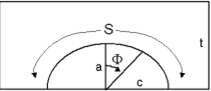
Normally, the Master Curve parameters are determined using test specimens with "straight" crack fronts and comparatively uniform stress state along the crack front. This enables the use of a single KI value and single constraint value to describe the whole specimen. For a real crack in a structure, this is usually not the case. Normally, both KI and constraint varies along the crack front and in the case of a thermal shock, even the temperature will vary along the crack front. Generally real cracks are simplified in the form of ellipses in order to aid the analysis. An example of an elliptic surface crack is shown Fig. 2.
The standard Master Curve cumulative failure probability expression is of the form:
−
−
⋅
−
=
4 min 0 min 0exp
1
K
K
K
K
B
B
P
If (1)
where B is the specimen thickness, B0 is the normalization thickness 25 mm, Kmin is the minimum fracture toughness 20 MPa√m, KI is the crack driving force and K0 is the fracture toughness corresponding to 63.2 % failure probability.
For a real three dimensional crack, both KI and K0 may vary as a function of location (Φ) along the crack front. This leads to the need of a more general expression for the cumulative failure probability (Eq. 2). The expression gives the cumulative failure probability, but it is not suited for a simple visualization of the result.
⋅
−
−
−
=
∫
Φ Φ s I fB
ds
K
K
K
K
P
0 0 4 min 0 minexp
1
(2)A visualization, that is in line with present structural integrity practice, can be achieved by defining an effective stress intensity factor KIeff corresponding to a specific reference temperature. The reference temperature can, for example, be chosen as the minimum temperature along the crack front. The procedure is to determine an effective driving force, which would give the same failure probability as Eq. 2, in the context of a standard Master Curve presentation. This means essentially a combination of Eqs. 1 and 2. The result is presented in Eq. 3.
(
0 min)
min4 / 1 0 0 4 min 0 min
K
K
K
B
ds
K
K
K
K
K
Tref s IIeffTref
⋅
−
+
⋅
−
−
=
∫
Φ Φ (3)KIΦ is obtained from the stress analysis as a function of location (Φ. K0Tref is the standard, high constraint, Master Curve K0, corresponding to a reference temperature along the crack front and it has the form
(
)
[
0]
0
31
77
exp
0
.
019
T
T
K
Tref=
+
⋅
⋅
ref−
(4)K0Φ is the local K0 value, based on local temperature and constraint. It can be expressed either as (Wallin, 2004)
°
−
−
−
⋅
⋅
+
=
=
− − = ΦC
MPa
stress
T
T
T
K
K
TT stress T stress/
12
019
.
0
exp
77
31
0, 0, 0
0 (5a)
or (Wallin, 2001)
°
−
−
−
⋅
⋅
+
=
=
− ΦC
MPa
stress
T
T
T
K
K
TT stress deep/
10
019
.
0
exp
77
31
0 , 00 (5b)
Out of the two expressions, Eq. 5b is also directly applicable with the ASME Code Case N-629 (or N-631) fracture toughness reference curve, since it is written in terms of the standard deep specimen T0. Eq. 5a makes use of the zero T-stress value of T0. This is a more sophisticated method, but relies on a non-standard definition of T0. At present Eq. 5b is therefore the more practicable form.
Eqs. 3 to 5 give the effective crack driving force, normalized to represent a standard Master Curve 25 mm crack front (B0) and the minimum temperature along the crack front.
(
)
[
ref deep]
Tref
T
T
K
5%,=
25
.
2
+
36
.
6
⋅
exp
0
.
019
⋅
−
0 (6)or by using the fracture toughness reference curve from ASME Code Case N-629 (or N-631). This can be expressed in the form
(
)
[
ref deep]
TrefASME
IC
T
T
K
− ,=
36
.
5
+
11
.
4
⋅
exp
0
.
036
⋅
−
0 (7a)or
(
)
[
T
RT
C
]
K
IC−ASME,Tref=
36
.
5
+
3
.
1
⋅
exp
0
.
036
⋅
ref−
To+
55
.
5
°
(7b)The resulting visualization is presented in Fig. 3. The difference to the presently used visualization is that the fracture toughness is not directly compared to the crack driving force estimated from stress analysis. Instead, the fracture toughness is compared to an effective driving force, which accounts for the local stress and constraint state and temperature along the crack front, as well as the crack front length. This way it is possible to combine the classical way of fracture mechanical analysis and state of the art Master Curve analysis, and presenting the analysis result in a conventional format.
-50 0 50 100 150 200
0 50 100 150 200 250
KIe
ff
, K
IC
[MPa
√
m]
Tmin-T0deep [oC]
KIC
5% MC
KIC, N-629
KIeff
Fig. 3. Principle of visualizing Master Curve analysis of real flaws.
The one thing to remember, however, is that postulated flaws often contain unrealistically long crack fronts. A quarter thickness flaw assumption may be justified, purely from a driving force perspective (as originally has been the intention). From a statistical size adjustment point of view, the assumption is over-conservative. If such postulated flaws are analyzed using KIeff, an additional size adjustment is recommended. A more realistic maximum crack front length is 150 mm. This value is also in line with the original KIC data used to develop the ASME KIC reference curve and therefore justifiable in terms of the functional equivalence principle. The form of KIeff for an excessively large postulated flaw (s > 150 mm) becomes thus
(
0 min)
min4 / 1
0 0
4
min 0
min
150
K
K
K
s
B
ds
mm
K
K
K
K
K
Trefs I
IeffTref
⋅
−
+
⋅
⋅
⋅
−
−
=
∫
Φ Φ
where the postulated crack front length (s) is replaced by a maximum crack front length of 150 mm. If NDE can guarantee a smaller value of s than 150 mm, it can be reduced further.
If warm pre stress (WPS) transients need to be analysed, they can be assessed based on the maximum KI along the crack front and Eqs. 6 or 8 or 7 (Wallin 2003).
3. MASTER CURVE ANALYSIS OF TSE-7
TSE-7 was an experiment involving a semi-elliptical surface flaw (Cheverton et al., 1985). The intention was to have a semicircular flaw with depth 19 mm and width 38 mm. After testing the flaw was found to have been irregular in shape, having a depth of only 14 mm with the exception of one local spike where the depth was 19 mm as shown in Fig. 4 (Cheverton et al., 1985). This irregularity was disregarded in the analysis and the flaw was simply modeled as a semi-ellipse. The shape of the crack was such that the KI value estimated by the original analysis is likely to slightly underestimate the actual situation in the test. The interpretation of the test is disturbed by the fact that neither KI nor T is constant along the crack front. The assessment should therefore be made in terms of KIeff, as described above. After first initiation, two additional initiations occurred. The problem is that strong bifurcation occurred all along the cylinder surface, making an accurate estimation of both actual KI as well as effective crack front length, practically impossible as seen from Fig. 5 (Cheverton et al., 1985). Therefore, only the first initiation was included in the detailed evaluation.
0 10 20 30 40
SIZE (mm) Surface 20
10
0
DEPTH (mm)
KW2335
Fig. 4. Actual crack profile of TSE-7 (Cheverton et al., 1985).
Fig. 5. Surface bifurcation pattern of TSE-7 (Cheverton et al., 1985).
two locations where the fracture surface indicated cleavage initiation (Fig. 8, Cheverton et al., 1985). The original report gives the KI value corresponding to the 5 mm location (T = -55ºC) as the primary initiation site, but also the other location is included in Fig. 7, since this value would be used for a simplified safety assessment, which combines minimum temperature with maximum KI. As seen by the results, also a simplified standard safety analysis without any size adjustments would lead to a fully acceptable assessment. This is a direct consequence of the crack being of a realistic size.
-15 -10 -5 0 5 10 15
-80 -60 -40 -20 0 20 40 60
KI
[MPa
√
m],
a
mm], T
[
o C]
c?[mm] TSE-7 at first initiation
a KI
T
Fig. 6. Temperature and stress intensity distribution along crack front at moment of
cleavage initiation for TSE-7.
-100 -80 -60 -40 -20 0 20
0 50 100 150 200
KIC N-629
K Ieff
, K
IC
[MP
a
√
m]
T [oC] TSE-7 KIeff
Based on actual flaw, stress and temperature
distributions. K
IC 5% MC
Local T and K
I
close to initiation sites
FLAW
INITIATION SITES
Fig. 8. Cleavage initiation sites in TSE-7 (Cheverton et al., 1985).
.
4. MASTER CURVE ANALYSIS OF PTSE-1 AND PTSE-2
As a final example of the Master Curve analysis of real cracks, including also the T-stress based constraint sensitivity equation (Eq. 5 a and b), two large scale experiments were analyzed based on the Master Curve methodology. The experiments studied were the pressurized thermal shock experiments PTSE-1 and PTSE-2 performed at ORNL national laboratory (Bryan et al., 1985, Bryan et al., 1987). The tests were performed on two large scale pressure vessels with a wall thickness of 150 mm and with 1 m long surface cracks. The initial flaw depth in both cases was close to a/W = 0.1. The pressure vessels experienced real pressurized thermal shocks. PTSE-1 experienced three different transients and PTSE-2 two. In both tests, both brittle crack initiation and arrest occurred. The tests are up to date, the ones most closely mimicking a real PTS transient in a nuclear pressure vessel. Until now, the experiments have not been analyzed with the Master Curve methodology.
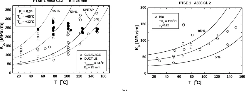
The material for PTSE-1 was a SA-508 class 2 steel with Yield stress = 625 MPa, Ultimate stress = 785 MPa, NDT = +66ºC and RTNDT = +91ºC (Bryan et al., 1985). The cleavage fracture initiation properties of the steels turned out to be strongly inhomogeneous. This required a non-standard inhomogeneous bimodal Master Curve analysis of the material (Wallin et al, 2004). The resulting MC analysis is presented in Fig. 9a. The fracture toughness was measured using 25 mm C(T) specimens, so their T-stress/σYT is about 0.4. The material can be divided into two different fracture toughness populations. One, with a T0 of +65ºC with an occurrence probability of 34 % and an other with a T0 of 12ºC with an occurrence probability of 66 %. Since the flaw in the experiment was 1000 mm in length, a value of +65ºC was taken as descriptive of the material. Similarly, the crack arrest test results were analyzed with a similar but simpler log-normal distribution having the same temperature dependence as the MC. The analysis indicated a transition temperature of +113ºC for the median crack arrest toughness of 100 MPa√m.
The material for PTSE-2 was an A 387 grade 22 class 2 steel (Bryan et al., 1987). The pre-test values were: Yield stress =280 MPa, Ultimate stress = 575 MPa, NDT = +49ºC, (RTNDT = 99ºC). In the test, the low yield strength caused the steel to plastify and this affected the mechanical properties. The post-test values were: Yield stress =470 MPa, Ultimate stress = 625 MPa, NDT = +75ºC. The pre- and post-test fracture toughness is presented in Fig. 10. Also here, the fracture toughness characterization used 25 mm C(T) specimens. There is a clear difference between the two material states. However, the PTSE-2 material does not show the same inhomogeneity as PTSE-1. This enabled a standard MC analysis of the data.
a)
20 40 60 80 100 120 140 160
0 50 100 150 200 250 300 350 P
a = 0.34
T01 = +65o
C
T02 = +12o
C
SINTAP 50 %
5 % 95 %
PTSE-1 A508 Cl.2 B = 25 mm
CLEAVAGE DUCTILE
T0SINTAP = 34
o
C
B0 = 25 mm
KJC
[M
Pa
√
m]
T [oC]
b)
20 40 60 80 100 120 140 160
0 50 100 150 200 5 % 95 % PTSE 1 A508 Cl. 2
KIa
TKIa = 113
o
C
σd=0.26
KIa
[MP
a
√
m]
T [oC]
Fig.9. Initiation and arrest fracture toughness for the PTSE-1 material.
a)
-80 -60 -40 -20 0 20 40 60 80
0 50 100 150 200 250 300 350
M = 30
5 % 95 % PTSE2 Pretest σY = 280 MPa B = 25 mm CT
CLEAVAGE
T
0 = 28 o
C
B0 = 25 mm
KJC
[M
Pa
√
m]
T [oC]
b)
0 20 40 60 80 100
0 50 100 150 200 250 300
M = 30
5 % 95 %
PTSE2 Posttest σY = 470 MPa B = 25 mm CT
CLEAVAGE
T
0 = 53 o
C
B0 = 25 mm
KJC
[M
Pa
√
m]
T [oC]
Fig.10. Initiation fracture toughness for the PTSE-2 material.
a)
-100 -50 0 50 100
0 50 100 150 200 250 5 % 95 % PTSE-2 Pretest
KIa
TK
Ia = 69 o C σ d=0.18 KIa [MPa √ m]
T [oC]
b)
-40 -20 0 20 40 60 80 100 120
0 50 100 150 200 5 % 95 % PTSE-2 Posttest
KIa
TK
Ia = 91 o
C
σd=0.16
KIa
[MP
a
√
m]
T [oC]
Fig. 11. Crack arrest fracture toughness for the PTSE-2 material.
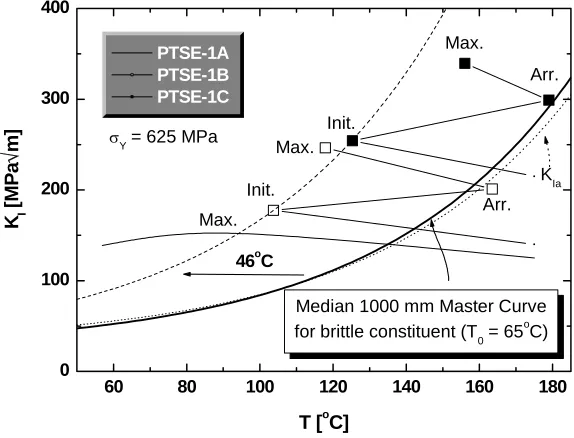
describe very well the crack arrest events in the tests. This means that standard crack arrest toughness is directly applicable to describe crack arrest of a component. The same is not the case for the initiation fracture toughness.
60 80 100 120 140 160 180
0 100 200 300 400
KIa
σY = 625 MPa
Max.
Max.
Max.
Arr.
Arr. Init.
Init.
46oC
Median 1000 mm Master Curve for brittle constituent (T
0 = 65
o C)
KI
[M
P
a
√
m]
T [oC]
PTSE-1A PTSE-1B PTSE-1C
Fig. 12. Transients of PTSE-1.
60 80 100 120 140 160
0 100 200 300 400
KIa
WPS
σY = 280 MPa
Arr.
Arr. Arr.
Init.
Init.
26oC
Median 1000 mm Master Curve
(T0 = 28oC)
KI
[M
P
a
√
m]
T [oC]
PTSE-2A PTSE-2B
Fig. 13. Transients of PTSE-2
additionally affected by a warm pre-stress effect in transient 2A. This can be accounted for by using a simple equation described in (Wallin, 2003). The T-stress for the C(T) specimens is approximated based on the yield stress at +100ºC as approximately 230 MPa for PTSE-1 and 100 MPa for PTSE-2. The T-stresses for the pressure vessels were estimated from the measured KI values together with crack depth and biaxiality (β-values for a SE(T) specimen. The shallow flaw SE(T) specimen is expected to provide a good estimate of the pressure vessel constraint in these tests. The estimate for PTSE-1 is approximately -350 MPa and for PTSE-2 approximately -270 MPa. This means that the T-stress difference for PTSE-1 is of the order of 580 MPa and for PTSE-2 of the order of 370 MPa. When these values are put into Eq. 5a, the resulting expected shift in T0 is for PTSE-1 48ºC and for PTSE-2 31ºC. These predictions comply extremely well with the shifts estimated directly from the tests (46ºC for PTSE-1 and 26ºC for PTSE-2).
A further analysis of the tests was performed using the procedure described above. The expression for KIeff is simplified, since the temperature and KI are constant along the crack front. Thus, an integration of Eq, 3 is not required. In order to enable a direct comparison with the ASME Code Case N-629, Eq. 5b was used for the constraint adjustment. This produces an additional degree of safety since the C(T) specimens are assumed to represent zero T-stress. If SE(B) specimens would have been used, the additional degree of safety would decrease, but not disappear. The resulting analysis result is presented in Fig. 14. The failure values are located approximately 15ºC above the 50 % Master Curve prediction. This represents the additional degree of safety resulting from combination of C(T) specimen data with Eq. 5b. The ASME Code Case N-629, including the size adjustment and accounting for constraint, provides a clearly conservative estimate of the PTSE tests.
-40 -20 0 20 40 60 80 100
0 100 200 300 400
KIe
ff
[MPa
√
m]
T-T0 [oC] PTSE-2
PTSE-1
PTSE-1 (non failure)
ASME N-629 50 % MC
Fig. 14. ORNL PTSE tests analysed according to Master Curve concept.
The above examples show how the Master Curve concept can be applied to real cracks in an optimum way. If the real crack front length is very long, the Master Curve requires it to be size adjusted accordingly, however, if postulated cracks are assessed, the size adjustment is normally not required or it can be limited to 150 mm as shown in Eq. 8.
-40 -20 0 20 40 60 80 100 0
100 200 300 400
ASME N-629 PTSE-2
PTSE-1
PTSE-1 (non failure)
KJC
[MP
a
√
m]
T-T0 [oC]
Unadjusted data
Fig.15. Application of the ASME Code Case N-629 to unadjusted PTSE data.
5. SUMMARY AND CONCLUSIONS
Normally, the Master Curve parameters are determined using test specimens with "straight" crack fronts and comparatively uniform stress state along the crack front. This enables the use of a single KI value and single constraint value to describe the whole specimen. For a real crack in a structure, this is usually not the case. Normally, both KI and constraint varies along the crack front and in the case of a thermal shock, even the temperature will vary along the crack front. A proper means of applying the Master Curve methodology for such cases has been presented here. Two examplatory analyzes, one for TSE-7 with an elliptical surface flaw and one for the PTSE-1 and PTSE-2 tests with long cracks, highlight the power of the methodology and provide strong validation for it. At the same time, the KIa Master Curve has been validated.
REFERENCES
Bryan, R. H., et al., (1985), "Pressurized-Thermal-Shock test of 6-in. thick pressure vessels. PTSE-1: Investigation of warm prestressing and upper-shelf arrest", NUREG/CR-4106, Oak Ridge National Laboratory. Bryan, R. H.,et al., (1987), "Pressurized-thermal-shock test of 6-in.-thick pressure vessels. PTSE-2: investigation of low tearing resistance and warm prestressing", NUREG/CR-4888, Oak Ridge National Laboratory.
Cheverton, R. D., et al., (1985), "Pressure vessel fracture studies pertaining to the PWR thermal-shock issue: Experiment TSE-7", NUREG/CR-4304, Oak Ridge National Laboratory.
Wallin, K., (1999), Int. J. of Materials and Product Technology, Vol. 14, pp-342-354. Wallin, K., (2001), Engng. Frac. Mech., Vol 68, pp. 303-328.
Wallin, K., (2003), Engng. Frac. Mech., Vol 70, pp. 2587-2602.
Wallin, K., (2004), "Experimental estimation of constraint", VTT Research report BTUO72-041227.