Retrieval of Refractivity Profile with Ground-Based Radio
Occultation by Using an Improved Harmony Search Algorithm
Mu-Min Chiou and Jean-Fu Kiang*
Abstract—A ground-based radio occultation (RO) technique is proposed to retrieve the atmospheric refractivity profile around a specific region at a higher sampling rate than conventional space-based RO techniques, making it more suitable for regional weather studies. A harmony search (HS) algorithm with ensemble consideration (HS-EC) based on atmospheric physics is proposed to retrieve the refractivity profile more efficiently without being trapped in suboptimal solutions. The highest altitude of profile is extended to 95 km from 40 km adopted in conventional ground-based RO techniques, leading to more accurate results.
1. INTRODUCTION
The height profile of refractivity used to be retrieved by using space-based radio occultation (RO) technique [1, 2], where excess phase-paths of GPS signals received at low-earth orbit (LEO) satellites and the bending angles of ray paths were used to reconstruct a height profile of refractivity via Abel transform [3, 4]. Global coverage of refractivity profiles is useful to predict weather conditions in the troposphere and the lower stratosphere [5, 6], to study heavy precipitation [7], Arctic atmosphere [8], severe weather events [9, 10], and over-the-horizon communication channels [11].
The space-based RO technique becomes less accurate in the lower troposphere, especially when a super-refraction (SR) layer is present [12], which happens frequently above sea surfaces [13]. Currently available space-based RO missions can provide only relatively sparse data for any specific region of interest [14], which is not sufficient for regional weather studies. A tomography technique was applied to retrieve meteorological profiles in the atmosphere by deploying a dense network of GPS receivers [15]. However, to monitor the temporal and spatial variations around a specific region demands even more receivers [16].
Ground-based RO technique was proposed for regional weather studies, which demanded a high sampling rate [14, 17]. A practical ground-based RO technique can be implemented at a specific site, by installing a receiver on building roof, vehicle or ship [18]. A ray-tracing model was applied to retrieve the atmospheric refractivity profile from the measurement data of GPS tropospheric delays [19]. In [20], a three-level model was proposed to characterize the ducting conditions near coast. Temporal and spatial variations in temperature, pressure and water vapor create a volatile refractivity profile, making its retrieval a challenging task. In [21], GPS signals at a specific ground-based receiver were used to retrieve height profile of maritime refractivity by using an artificial neural network technique, which was validated by measurement data on the coast of the Yellow sea.
In [18], an exhaustive search (ES) method was applied to retrieve the refractivity profile from the boundary layer up to 10 km above ground, with data from a single ground-based GPS receiver. The computational time of the exhaustive search method grows exponentially with the number of
Received 25 May 2016, Accepted 24 August 2016, Scheduled 14 October 2016 * Corresponding author: Jean-Fu Kiang ([email protected]).
unknowns [22]. To reduce the size of search space, variable searching steps were taken at different heights, and the data of the Constellation Observing System for Meteorology, Ionosphere, and Climate (COSMIC) mission from 2007 to 2011 were used as prior information [23]. A harmony search (HS) algorithm, inspired by the improvisation process of Jazz musicians, was proposed to search for the optimal solution more efficiently [24]. To avoid being trapped in local optimal solutions, ensemble consideration was implemented to constrain the solution vector to resemble a preferred pattern.
In this work, we will first demonstrate that more accurate data of excess phase-path are critical to the effectiveness of a ground-based RO technique. In order to obtain more accurate excess phase-paths, the upper bound of integration assumed in the ray-tracing model should be increased. An HS algorithm with ensemble consideration (HS-EC) based on atmospheric physics is proposed to retrieve the refractivity profile, which contains more unknowns than the conventional exhaustive search method can handle at a reasonable computational load.
This paper is organized as follows. A ray-tracing model is briefly reviewed in Section 2. The significance of integration upper bound on computing the excess phase-path is analyzed in Section 3. The HS-EC algorithm based on atmospheric physics is presented in Section 4. Simulation results are discussed in Section 5. Finally, some conclusions are drawn in Section 6.
2. RAY-TRACING MODEL IN GROUND-BASED RO
In this section, some basic concepts of ray tracing and the retrieval algorithm applied in ground-based RO are briefly reviewed. Figure 1 shows the geometry of a ray path in a scenario of ground-based radio occultation [20], where A1 and A2 represent a GPS receiver on the ground and a GPS satellite,
respectively; with their distances to the Earth center beingr1 and r2, respectively.
Figure 1. Geometry of ray path in ground-based radio occultation [20].
If the atmospheric profile is approximated as a function of r only, the phase-path between points
A1 and A2 is determined as
S = A2
A1
nd, (1)
whered =√dr2+r2dθ2=dr/cosφis a differential length along the ray path, andn is the refractive
index. In practice, a refractivity is defined as N = 106 ×(n−1), which can be empirically estimated as [18]
N =k1
P T +k2
Pw
T2, (2)
wherek1= 77.6 (N-unit×K/hPa) andk2 = 3.73×10⁵ (N-unit×K2/hPa);P (hPa), Pw (hPa) and T
(K) are the atmospheric pressure, water-vapor pressure and temperature, respectively.
A ray path in a spherically symmetric medium follows the Bouger’s law,a=nrsinφ, whereais a constant impact parameter associated with the ray path. Thus, Eq. (1) can be represented as
S= r2
r1
rn2
√
r2n2−a2dr=
x2
x1
x[1−(x/n)dn/dx]
√
where x =rn is called the refractional radius. The phase-path along a straight line between A1 and
A2, as if they were in vacuum, can be determined as
S0=
r21+r22−2r1r2cosθ0, (4)
whereθ0 is the angle span betweenOA1 and OA1.
An excess phase-path is defined as [20]
ΔS =S−S0, (5)
and the elevation angleβ is determined as
β = tan−1r2cosθ0−r1
r2sinθ0
. (6)
As the satellite moves in its orbit, many ray paths are established between A1 and A2, with each ray
path associated with an elevation angle β and an excess phase-path ΔS. The information of N(h) is embedded in these pairs of (ΔS, β)’s, which can be transformed to a functional form of ΔS(β) by applying a cubic-spline interpolation [20]. The retrieved refractivity can be determined by fitting the modeled excess phase-path ΔSmod(β) with the measured excess phase-path ΔSmea(β) in the least-square sense as
Nre(h) = arg min
N(h)
M o
m=1
ΔSmea(βm)−ΔSmod(βm) 2
, (7)
whereMo is the number of measurement data, and h=r−Re is the height above ground.
The effects of horizontal refractivity gradient, multipath and atmospheric diffraction are neglected atβ >3◦. Whenβ >5◦, the variation of ΔSover different refractivity profiles becomes insignificant [25]. Hence, the range of elevation angle in this work is chosen to be 3◦ ≤β ≤5◦ [18].
3. EFFECT OF UPPER BOUND ON EXCESS PHASE-PATH
In this section, the effect of upper bound in the integral is studied, with practical atmospheric profiles. Figure 2 shows the geometry of a ray path for computing the phase-path fromA1 toA2 via Au, above
which the refractive index is approximated as one. The point Au is at a distance of ru from the Earth center, or is at a height of hu =ru−r1 above ground. Let the phase-path betweenA1 and Au beS1u,
and that betweenAu andA2 beSu2. Thus, the phase-path integration in Eq. (3) is divided to two parts
as
S= xu
x1
x[1−(x/n)dn/dx]
√
x2−a2 dx+
x2
xu
x[1−(x/n)dn/dx]
√
x2−a2 dx, (8)
where the two terms on the right-hand side are S1u and Su2, respectively, and xα = nαrα is the
refractional radius atAα, withα= 1,2, u. Since the refractive index abovehu is approximated as one,
Su2 can be approximated as
Soa=
x2
2−a2− x2u−a2.
Figure 3. Profile of excess phase-path ΔS, at 00:00 UTC, Jan. 1, 2014, (23.5◦N, 120◦E), r1 =
6,400 km, r2 = 26,600 km,a= 6,396.984 km.
Figure 4. Excess phase-path versus elevation angle in two refractivity profiles at latitudes 0◦ and 90◦N, respectively, derived from the zonal average pressure and temperature of the CIRA86aQ UoG model in January [26].
By using Eqs. (4), (5) and (8), a relation between the excess phase-path ΔS andhu is obtained, as shown in Figure 3. Note that ΔS(hu) increases withhu and approaches a constant when hu >90 km.
Figure 4 shows the excess phase-path as a function of elevation angle, in two refractivity profiles at latitudes 0◦ and 90◦N, respectively [26]. The difference between these two excess phase-paths is about 5 m at all elevation angles. Other parameters like slant delays and slant factors involved in a typical ray-tracing method were discussed in [27]. However, the minimum altitude required to acquire accurate phase-paths was not conclusive for ground-based RO techniques, and 40 km was frequently adopted as the upper bound of integration for computing phase-paths [18].
Figure 3 shows that as hu is changed from 40 km to 90 km, the excess phase-path is changed by about 0.7 m, which is about 1/7 of the difference between the two curves in Figure 4. This implies if
hu is set to 40 km, one may not be able to tell apart the excess phase-paths in two different refractivity profiles. In this work, the upper bound is raised to 95 km, above which the refractive index is much closer to one than at 40 km above ground.
The air pressure, water-vapor pressure and temperature can be derived from the European Centre for Medium-Range Weather Forecast (ECMWF) model [28]. However, the ECMWF model and the COSMIC mission [23] provide atmospheric data only up to 50 km above ground. Hence, the CIRA86aQ UoG model [26] and the MSIS-E-90 model [29] are adopted to provide the pressure and temperature profiles up to the altitude of 95 km.
4. HARMONY SEARCH ALGORITHM WITH ENSEMBLE CONSIDERATION ON ATMOSPHERIC PHYSICS
In this Section, the HS-EC algorithm tailored for ground-based RO missions is presented. 4.1. Harmony Search Algorithm
The harmony search (HS) algorithm updates the solution set stored in a harmony memory (HM), which can be represented as [24, 30]
HM = ⎡ ⎢ ⎢ ⎣
N11 N21 . . . NHMS1
N12 N22 . . . NHMS2
..
. ... . . . ...
N1M N2M . . . NHMSM
⎤ ⎥ ⎥ ⎦,
Figure 5. Refractivity profile {Nm} sampled at altitudes{hm}, with 1≤m≤M.
Figure 6. Refractivity profiles in January derived from the CIRA86aQ UoG model.
vector having a smaller object function value is placed before those having larger object function values. Figure 5 shows an example of refractivity profile, which is represented by the best harmony vector to be, ¯N = [N1, N2, . . . , NM]t, whereNm is the refractivity at height hm.
Figure 6 shows three refractivity profiles over the heights from 0 to 100 km, which are obtained by applying Eq. (2), where the zonal average pressure and temperature are derived from the CIRA86aQ UoG model [26]. These curves can be fit with logarithmic-like functions as [18]
N(h) =Nmexp
− h−hm
hm+1−hm
ln Nm
Nm+1
, hm≤h≤hm+1.
In each improvisation, the HS algorithm is implemented in five steps, which are briefly described as follows.
Step 1, random selection process:
In the beginning of the th improvisation, a new harmony vector ¯N() is generated, with its mth entry picked from an interval as
Nm()=U(NmL, NmU), (9) whereU(α, β) represents a uniform distribution over the interval (α, β);NmL and NmU are the lower and upper bounds, respectively, ofNm, which are also marked in Figure 5.
Step 2, memory consideration process:
An alternative new harmony vector ¯N() is generated as
Nm()=Npm, (10)
whereNpmis the pmth entry in the harmony memory, with
p=U2(0,1)×HMS+ 1, (11) where r means the integer part of a positive real number r. Steps 1 and 2 are executed with probabilities of 1-HMCR and HMCR, respectively.
Step 3, pitch adjustment process: The value ofNm() is pitch-adjusted as
Step 4, memory update process:
If ¯N() bears a smaller object function value than the worst harmony in the HM, the latter will be replaced with ¯N().
Step 5, accidentaling process:
If ¯N() is the best within the HM, it will be pitch-adjusted as
Nmac=Nm()+U(−1,1)×FWm, 1≤m≤M. (13) If ¯Nac bears a smaller object function value than the worst harmony in the HM, the latter will be
replaced with ¯Nac. The HS algorithm stops as the iteration indexreaches an upper boundK.
4.2. HS Algorithm with Ensemble Consideration
Refractivities Nm+1 and Nm, at adjacent heights, are strongly correlated because the atmospheric
variables P, T and Pw that determine the refractivity do not change drastically over a small height range. This fact can be used to guide the HS algorithm from converging to suboptimal solutions. It is implemented in the form of ensemble consideration (EC), in which the refractivities at adjacent height intervals, ¯Nm() and ¯Nm(+1) , are constrained to resemble the so called ensemble-consideration refractivities
¯
NmEC and ¯NmEC+1, respectively. The latter are derived by imposing atmospheric physics as in Step 1a below.
Figure 7 shows a flowchart of the HS-EC algorithm, in which the ensemble consideration is implemented in the processes of random selection, memory consideration, pitch adjustment and accidentaling. The processes enclosed in the dashed rectangle are used to generate a new harmony vector ¯N(), and K is an upper bound of iteration index . The four steps of the HS-EC algorithm are described as follows.
Step 1a, random selection process:
The measurement data on the ground is taken as N1, and the other ¯N()’s are generated as
Nm()=Nm()−1 N
EC m
NmEC−1 +c1×U(−1,1)×
NmU −NmL, 2≤m≤M, (14) wherec1 is a weighting coefficient, with a normal range from 0.01 to 0.1 [24]. Choosing a smallerc1 will
makeNm() closer to the ensemble-consideration refractivity profile in [hm−1, hm]. In the simulations,c1
is decreased linearly from an initial value c10 at = 1 to zero at =K.
The ensemble-consideration refractivity profile N¯EC is derived by using Eq. (2), with the temperatureT(h), pressureP(h) and water vaporPw(h) estimated as [26, 31]
T(h) = TC(h)−T0C+T0mea, P(h) = P0meaexp
−gma
R
h
0
dh T
,
Pw(h) = PwC(h)P
mea w0
PwC0 ,
where TC(h) and T0C are the temperature profile and the temperature on the ground, respectively, derived from the CIRA86aQ UoG model; T0mea is the measured temperature on the ground, P0mea the measured pressure on the ground, R = 8.31451×104cm3hPa/mole/K the atmospheric constant, and
ma = 0.028966 kg/mole the molecular weight averaged over N2, O2, Ar and CO2 in a standard model;
PwC(h) and PwC0 are derived from the CIRA86aQ UoG model, and Pwmea0 is the water-vapor pressure measured on the ground.
Step 2a, memory consideration process: Themth entry ofN() is alternately generated as
Nm() =Nm(−)1 Npm Np(m−1)
, (15)
where p is determined by using Eq. (11). Steps 1a and 2a are executed with probabilities of 1-HMCR and HMCR, respectively.
Step 3a, pitch adjustment process: The value ofNm() is pitch-adjusted as
Nm()=Nm()+c1×U(−1,1)×
NmU−NmL, (16) with a probability of PAR.
Step 5a, accidentaling process:
If ¯N() is the best within the HM, it will be pitch-adjusted as
Nmac=Nm()+c2×U(−1,1)×
NmU−NmL, 1≤m≤M, (17) where c2 is a weighting coefficient to fine-tune the best candidate solution. The value of c2 is usually
smaller than c1 and is decreased linearly fromc20 at = 1 to zero at =K. The idea of decreasingc1
and c2 is to encourage exploration in the early stage while accelerate convergence in the late stage [32].
In practice, a negative refractivity may occur at high altitudes due to the random term c1 ×
U(−1,1)×(NmU−NmL) in Eqs. (14) and (16), because the modeled refractivity generated with Eqs. (14) and (15) decreases moronically with height, and a smallNm tends to generate an even smaller Nq with
q≥m+ 1. This issue can be resolved by imposing the ensemble consideration. 5. SIMULATIONS AND DISCUSSIONS
from the ECMWF model. The maximum error of excess phase-path in ground-based measurements was about 15 cm [20, 33]. In this work, the simulated excess phase-path is the sum of the actual excess phase-path (ΔS) and a Gaussian noise with zero mean and standard deviation of 10−3ΔS [20].
To evaluate the quality of reconstructed refractivity profile, a root-mean-square (rms) percentage error is defined as
ε= 100×
1
hb−ha
ha
hb
|Nre(h)−Ntar(h)|2
|Ntar(h)|2 dh, (18)
where ha and hb are chosen to cover the troposphere and the lower stratosphere. The tropopause between the troposphere and stratosphere lies at the height of about 18 km near the equator, about 10 km at mid-latitudes, and about 8 km at the poles.
In applying the HS algorithm, the number of unknowns in a profile was below 40 [34]. In order to retrieve the refractivity profile from ground up to 95 km at height, without involving too many unknowns, the refractivity profile is sampled with a finer resolution at lower altitudes and a coarser resolution at higher altitudes. Table 1 lists two altitude schemes, with Δhindicating altitude resolution. In scheme 1, the sampling interval is 0.5 km in 0≤h≤10 km, 2 km in 10≤h≤20 km, 5 km in 20≤h≤75 km, and 10 km in 75≤h≤95 km, adding up to 39 height levels. In scheme 2, the sampling interval is 1 km in 0 ≤h≤10 km, 2 km in 10 ≤h≤20 km, 5 km 20 ≤h ≤75 km, and 10 km in 75≤ h≤95 km, adding up to 29 height levels.
Table 1. Two altitude schemes adopted in simulations.
altitude scheme 1 (39 levels)
altitude range (km) 0–10 10–20 20–75 75–95
Δh (km) 0.5 2 5 10
altitude scheme 2 (29 levels)
altitude range (km) 0–10 10–20 20–75 75–95
Δh (km) 1 2 5 10
5.1. Comparison between HS-EC and ES
Firstly, the HS-EC algorithm will be compared with the conventional exhaustive search (ES) method, with altitude scheme 2 listed in Table 1. A refractivity profile at (23◦N, 120◦E), 00:00 UTC, Jan. 1, 2013 is generated as the target refractivity profile, Ntar. The temperature and pressure profiles are derived from the MSIS-E-90 model, and the water-vapor pressure profile is derived from the ECMWF model.
Table 2 lists the rms percentage error averaged over 100 realizations by using the ES [18] and the HS-EC algorithms, respectively, and each is tested with different hu’s. The parameters used in the HS-EC algorithm are HMS = 20, HMCR = 0.9, PAR = 0.7,c10= 0.1 and c20= 0.01.
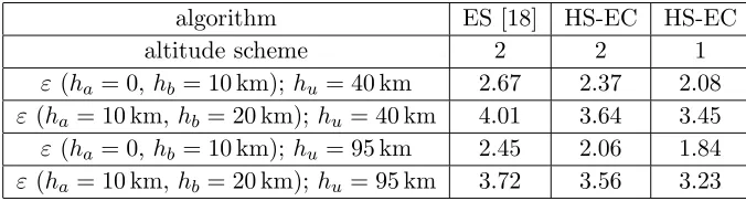
Table 2. Average rms percentage error of ES and HS-EC.
algorithm ES [18] HS-EC HS-EC
altitude scheme 2 2 1
ε(ha= 0,hb = 10 km);hu = 40 km 2.67 2.37 2.08
ε(ha= 10 km, hb= 20 km);hu= 40 km 4.01 3.64 3.45
ε(ha= 0,hb = 10 km);hu = 95 km 2.45 2.06 1.84
It is observed that the average rms percentage error is higher with (ha= 10 km, hb = 20 km) than that with (ha = 0, hb = 10 km). The refractivity decreases with height, and a fixed absolute error (Nre(h)−Ntar(h)) will result in a higher rms percentage error according to the definition in Eq. (18). By increasinghu from 40 km to 95 km, with altitude scheme 2, the average rms percentage error slightly decreases from 2.67 to 2.45 by using the ES method, and from 2.37 to 2.06 by using the HS-EC algorithm. The retrieved profile withhu = 95 km appears more accurate than that withhu= 40 km because more accurate excess phase-paths are available in the former case by including information from the upper atmosphere. If altitude scheme 1 is adopted, which defines a finer vertical resolution in the altitude range of 0–10 km, the average rms percentage error by using the HS-EC algorithm withhu= 95 km can be further reduced to 1.84.
Given the number of excess phase-paths (M) required in one mission, the computational load of the ES method is on the order ofqM, whereq is the number of candidate values at each height interval, usually larger than 10 [18]. As a result, the computational load with altitude scheme 1 will become too huge to be practical. That could be the reason why the ES method was often used with height intervals larger than 1 km [18]. On the other hand, the computational load of the HS or the HS-EC algorithm is on the order of 20,000, which is much smaller thanqM.
5.2. Comparison between HS-EC and HS
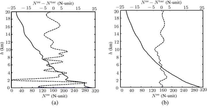
Figure 8(a) shows the retrieved refractivity Nre and errorNre−Ntar by using the HS algorithm, with the parameters HMS = 20, HMCR = 0.95, PAR = 0.5 and K = 20,000. The retrieved refractivity profile appears non-monotonical at heights around 1.8, 2.1 and 4.2 km, respectively, indicating thatNre
could be a suboptimal solution.
(a) (b)
Figure 8. Retrieved refractivityNre(———) and errorNre−Ntar (− − −) by using (a) HS algorithm and (b) HS-EC algorithm.
Figure 8(b) shows the retrieved refractivity profile and the error by using the HS-EC algorithm, with the parameters HMCR, PAR, HMS and K the same as in the HS algorithm, and the tuning parameters are c10 = 0.1 and c20 = 0.01. The retrieved refractivity profile appears monotonical, and
the errors are smaller than those in Figure 8(a).
5.3. Fine-Tune of HS Parameters
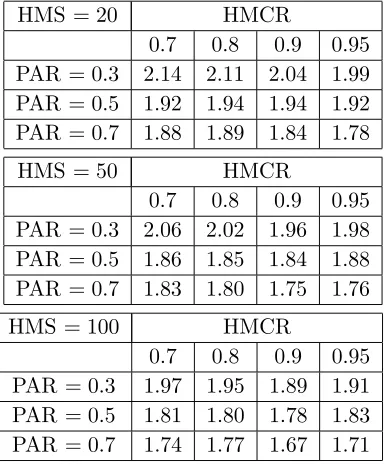
The accuracy of solution obtained with the HS-EC algorithm can be further increased by fine-tuning the relevant parameters. Table 3 lists the average rms percentage error over 100 realizations, with
K = 20,000, c10= 0.1,c20= 0.01, along with different combinations of HS parameters. It is concluded
that choosing HMS = 100, HMCR = 0.9 or 0.95, and PAR = 0.7 will achieve smaller rms percentage errors.
Table 3. Effects of HMS, HMCR and PAR on average rms percentage error,ha= 0, hb = 10 km.
HMS = 20 HMCR
0.7 0.8 0.9 0.95 PAR = 0.3 2.14 2.11 2.04 1.99 PAR = 0.5 1.92 1.94 1.94 1.92 PAR = 0.7 1.88 1.89 1.84 1.78
HMS = 50 HMCR
0.7 0.8 0.9 0.95 PAR = 0.3 2.06 2.02 1.96 1.98 PAR = 0.5 1.86 1.85 1.84 1.88 PAR = 0.7 1.83 1.80 1.75 1.76
HMS = 100 HMCR
0.7 0.8 0.9 0.95 PAR = 0.3 1.97 1.95 1.89 1.91 PAR = 0.5 1.81 1.80 1.78 1.83 PAR = 0.7 1.74 1.77 1.67 1.71
Table 4 lists the average rms percentage error over 100 realizations, withK = 20,000, HMS = 100, HMCR = 0.9, PAR = 0.7, along with different combinations of c10 and c20. Smaller rms percentage
errors can be achieved with 0.04≤c10≤0.1 and 0.007≤c20≤0.02.
Table 4. Effects ofc10 and c20 on average rms percentage error, ha = 0,hb = 10 km.
c10
0.005 0.01 0.04 0.07 0.1 0.2
c20= 0.001 1.89 1.81 1.75 1.74 1.75 1.79
c20= 0.004 1.84 1.76 1.72 1.73 1.73 1.74
c20= 0.007 1.83 1.73 1.71 1.68 1.69 1.72
c20= 0.01 1.84 1.72 1.70 1.69 1.67 1.70
c20= 0.02 1.86 1.73 1.71 1.72 1.69 1.74
c20= 0.03 1.87 1.75 1.76 1.71 1.71 1.71
c20= 0.04 1.88 1.74 1.74 1.72 1.77 1.76
In general, a largerc10gives more mobility in the early searching stage to avoid suboptimal solutions,
while a smaller c10 puts more weight on the ensemble-consideration refractivity ¯NEC. A smaller c20
forces the searching process to move in a smaller step, but the searching process may stall if c20 is too
small.
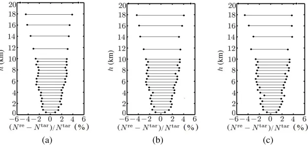
Figure 9 shows the percentage error, 100×(Nre−Ntar)/Ntar(%), at (0◦N, 0◦E), (30◦N, 0◦E) and
(a) (b) (c)
Figure 9. Percentage error, 100×(Nre−Ntar)/Ntar(%), by using HS-EC algorithm, (a) (0◦N, 0◦E), (b) (30◦N, 0◦E) and (c) (60◦N, 0◦E).
error range derived over 100 realizations. The error range is [−2.5,2.5]% below 10 km, and increases to [−6,6]% at altitude of 20 km. The absolute errors are smaller than 7 N-unit at all heights. As a comparison, the absolute error was about 10 N-unit in the lower troposphere when the ES method was applied [18].
6. CONCLUSION
A harmony search algorithm with ensemble consideration (HS-EC) based on atmospheric physics is applied to retrieve the refractivity profile in a specific area, from 0 to 95 km above the ground. Compared to conventional ground-based GPS retrieval techniques, the proposed method can retrieve more accurate refractivity profile partly because the upper bound of integration is extended to 95 km, and the measurement data at ground level are included. The ensemble consideration constrains the solution profile to resemble a standard profile, effectively guiding the solution from being trapped in suboptimal solutions, which may happen with the exhaustive search method or conventional HS algorithm, especially when the number of unknowns is large. The proposed method is capable of retrieving the refractivity profiles with a wider range of height and smaller height intervals, making regional weather studies more practical.
ACKNOWLEDGMENT
This work is sponsored by the Ministry of Science and Technology, Taiwan, ROC, under contract NSC 102-2221-E-002-043 and the Ministry of Education, Taiwan, ROC, under contract 105R3401-2.
REFERENCES
1. Liou, Y. A., A. G. Pavelyev, S. F. Liu, A. A. Pavelyev, N. Yen, C. Y. Huang, and C. J. Fong, “FORMOSAT-3/COSMIC GPS radio occultation mission: Preliminary results,” IEEE Trans. Geosci. Remote Sensing, Vol. 45, No. 11, 3813–3826, Nov. 2007.
2. Chiu, T. C., Y. A. Liou, W. H. Yeh, and C. Y. Huang, “NCURO data-retrieval algorithm in FORMOSAT-3 GPS radio-occultation mission,” IEEE Trans. Geosci. Remote Sensing, Vol. 46, No. 11, 3395–3405, Nov. 2008.
3. Kursinski, E. R., G. A. Hajj, W. I. Bertiger, S. S. Leroy, T. K. Meehan, L. J. Romans, et al., “Initial results of radio occultation observations of Earth’s atmosphere using the global positioning system,” Science, Vol. 271, No. 5252, 1107–1110, Feb. 1996.
5. Healy, S. B., A. M. Jupp, and C. Marquardt, “Forecast impact experiment with GPS radio occultation measurements,” Geophys. Res. Lett., Vol. 32, No. 3, L03804, Feb. 2005.
6. Le Marshall, J., Y. Xiao, R. Norman, K. Zhang, A. Rea, L. Cucurull, et al., “The application of radio occultation observations for climate monitoring and numerical weather prediction in the Australian region,”Aust. Meteorol. Oceanog. J., Vol. 62, 323–334, Sep. 2012.
7. Yang, S. C., S. H. Chen, S. Y. Chen, C. Y. Huang, and C. S. Chen, “Evaluating the impact of the COSMIC RO bending angle data on predicting the heavy precipitation episode on June 16, 2008 during SoWMEX-IOP8,” Month. Weather Rev., Vol. 142, No. 11, 4139–4163, 2014.
8. Pelliccia, F., F. Pacifici, S. Bonafoni, P. Basili, N. Pierdicca, P. Ciotti, and W. J. Emery, “Neural networks for arctic atmosphere sounding from radio occultation data,”IEEE Trans. Geosci. Remote Sensing, Vol. 49, No. 12, 4846–4855, Dec. 2011.
9. Zhang, K., T. Manning, S. Wu, W. Rohm, D. Silcock, and S. Choy, “Capturing the signature of severe weather events in Australia using GPS measurements,” IEEE Selected Topics Appl. Earth Observ. Remote Sensing, Vol. 8, No. 4, 1839–1847, Apr. 2015.
10. Norman, R. J., J. Le Marshall, W. Rohm, B. A. Carter, G. Kirchengast, S. Alexander, C. Liu, and K. Zhang, “Simulating the impact of refractive transverse gradients resulting from a severe troposphere weather event on GPS signal propagation,”IEEE Selected Topics Appl. Earth Observ. Remote Sensing, Vol. 8, No. 1, 418–424, Jan. 2015.
11. Chou, Y. H. and J. F. Kiang, “Ducting and turbulence effects on radio-wave propagation in an atmospheric boundary layer,” Progress In Electromagnetics Research B, Vol. 60, 301–315, 2014. 12. Sokolovskiy, S., “Effect of super refraction on inversions of radio occultation signals in the lower
troposphere,”Radio Science, Vol.38, No. 3, 24-1-14, Jun. 2003.
13. Von Engeln, A. and J. Teixeira, “A ducting climatology derived from the European centre for medium-range weather forecasts global analysis fields,”J. Geophys. Res. Atmos., Vol. 109, No. D18, D18104, Sep. 2004.
14. Zuffada, C., G. A. Hajj, and E. R. Kursinski, “A novel approach to atmospheric profiling with a mountain-based or airborne GPS receiver,” J. Geophys. Res. Atmos., Vol. 104, No. D20, 24435– 24447, Oct. 1999.
15. Flores, A., J. V.-G. De Arellano, L. P. Gradinarsky, and A. Rius, “Tomography of the lower troposphere using a small dense network of GPS receivers,”IEEE Trans. Geosci. Remote Sensing, Vol. 39, No. 2, 439–447, Feb. 2001.
16. Nilsson, T. and L. Gradinarsky, “Water vapor tomography using GPS phase observations: Simulation results,”IEEE Trans. Geosci. Remote Sensing, Vol. 44, No. 10, 2927–2941, Oct. 2006. 17. Lin, L. K., Z. W. Zhao, Y. R. Zhang, and Q. L. Zhu, “Tropospheric refractivity profiling based on refractivity profile model using single ground-based global positioning system,” IET Radar Sonar Navig., Vol. 5, No. 1, 7–11, 2011.
18. Wu, X., X. Wang, and D. L¨u, “Retrieval of vertical distribution of tropospheric refractivity through ground-based GPS observation,”Adv. Atmos. Sci., Vol. 31, No. 1, 37–47, Jan. 2014.
19. Sokolovskiy, S. V., C. Rocken, and A. R. Lowry, “Use of GPS for estimation of bending angles of radio waves at low elevations,” Radio Science, Vol. 36, No. 3, 473–482, May 2001.
20. Lowry, A. R., C. Rocken, S. V. Sokolovskiy, and K. D. Anderson, “Vertical profiling of atmospheric refractivity from ground-based GPS,” Radio Science, Vol. 37, No. 3, 13-1-19, Jun. 2002.
21. Wang, H. G., Z. S. Wu, S. F. Kang, and Z. W. Zhao, “Monitoring the marine atmospheric refractivity profiles by ground-based GPS occultation,”IEEE Geosci. Remote Sensing Lett., Vol. 10, No. 4, 962–965, Jul. 2013.
22. Nievergelt, J., “Exhaustive search, combinatorial optimization and enumeration: Exploring the potential of raw computing power,” Sofsem 2000: Theory and Practice of Informatics, 18–35, Springer, 2000.
23. Rocken, C., Y. H. Kuo, W. S. Schreiner, D. Hunt, S. Sokolovskiy, and C. McCormick, “COSMIC system descriptions,”Terr. Atmos. Ocean. Sci., Vol. 11, No. 1, 21–52, Mar. 2000.
25. Gaikovich, K. P. and M. I. Sumin, “Reconstruction of the altitude profiles of the refractive index, pressure, and temperature of the atmosphere from observations of astronomical refraction,”
Izvestiya, Atmos. Ocean. Phys., Vol. 22, 710–715, 1986.
26. Kirchengast, G., J. Hafner, and W. Poetzi, “The CIRA86aQ UoG model: An extension of the CIRA-86 monthly tables including humidity tables and a Fortran95 global moist air climatology model,”Euro. Space Agency, IMG/UoG Tech. Rep., Vol. 8. 1999.
27. Nafisi, V., L. Urquhart, M. C. Santos, F. G. Nievinski, J. Bohm, D. D. Wijaya, H. Schuh, A. A. Ardalan, T. Hobiger, and R. Ichikawa, “Comparison of ray-tracing packages for troposphere delays,” IEEE Trans. Geosci. Remote Sensing, Vol. 50, No. 2, 469–481, 2012.
28. Dee, D. P., S. M. Uppala, A. J. Simmons, P. Berrisford, P. Poli, S. Kobayashi, et al., “The ERA-interim reanalysis: Configuration and performance of the data assimilation system,” Q. J. R. Meterorol. Soc., Vol. 137, 533–597, Apr. 2011.
29. Hedin, A. E., “Extension of the MSIS thermosphere model into the middle and lower atmosphere,”
J. Geophys. Res. Space Phys., Vol. 96, No. A2, 1159–1172, Feb. 1991.
30. Yang, S.-H. and J.-F. Kiang, “Optimization of sparse linear arrays using harmony search algorithms,” IEEE Trans. Antennas Propagat., Vol. 63, No. 11, 4732–4738, Nov. 2015.
31. Jacobson, M. Z.,Fundamental of Atmospheric Modeling, Cambridge Univ. Press, 2005.
32. Ratnaweera, A., S. Halgamuge, and H. C. Watson, “Self-organizing hierarchical particle swarm optimizer with time-varying acceleration coefficients,” IEEE Trans. Evolution. Comput., Vol. 8, No. 3, 240–255, Jun. 2004.
33. Hajj, G. A., E. R. Kursinski, L. J. Romans, W. I. Bertiger, and S. S. Leroy, “A technical description of atmospheric sounding by GPS occultation,”J. Atmos. Solar-Terr. Phys., Vol. 64, No. 4, 451–469, 2002.
![Figure 1. Geometry of ray path in ground-based radio occultation [20].](https://thumb-us.123doks.com/thumbv2/123dok_us/1984483.1262332/2.612.254.364.379.487/figure-geometry-ray-path-ground-based-radio-occultation.webp)