Preliminary Results on Estimation of the Dispersive Dielectric
Properties of an Object Utilizing Frequency-Dependent
Forward-Backward Time-Stepping Technique
Shi W. Ng1, Kismet A. H. Ping1, *, Shafrida Sahrani1, Mohamad H. Marhaban2, Mohd I. Sariphan2, Toshifumi Moriyama3, and Takashi Takenaka3
Abstract—In this paper, a Frequency-Dependent Forward-Backward Time-Stepping (FD-FBTS) inverse scattering technique is used for reconstruction of homogeneous dispersive object. The aim of the technique is to reconstruct the relative permittivity at infinite frequency, static relative permittivity and static conductivity of the homogeneous dispersive object simultaneously. The technique utilizes iterative finite-difference time-domain (FDTD) method for solving inverse scattering problem in time domain. The minimization of the cost functional is carried out utilizing Dai-Yuan nonlinear conjugate-gradient algorithm. The Fr´echet derivatives of the augmented cost functional are derived analytically with respect to scatterer properties. Numerical results for reconstruction of two-dimensional homogeneous dispersive illustrate the performance of the proposed technique.
1. INTRODUCTION
Microwave tomography is an imaging technique which utilizes ultrawideband (UWB) microwave frequencies to solve an electromagnetic inverse scattering problem. This technique attracts significant interest for researchers due to the numerous applications in medical imaging [1–4], non-destructive evaluation [5–7], geophysical prospecting [8] and civil engineering [9]. In microwave tomography, low-power and short-duration microwave pulses will be transmitted from an array of antennas towards the scatterer, and the resulting scattered microwave signals are measured at the locations around the scatterer domain. The measurement data are then inverted in order to reconstruct the spatial distribution of the electromagnetic properties of the scatterer. The electromagnetic inverse scattering problem is nonlinear because scattered field is a nonlinear function of the scatterer properties. Moreover, the problem is an ill-posed problem where the ill-posedness appears as a result of the operator that maps the scatterer properties to the scattered field is compact.
The subject of great interest in microwave inverse scattering is the selection of the time-dependence of the incident fields. Besides this approach, there are many methodologies based on frequency-domain have been proposed [10–12]. In frequency-frequency-domain approach, the incidences are assumed to be monochromatic and the popular methods such as method of moments (MoM) [13, 14] and the finite-element method (FEM) [15], are utilized for field analysis of the frequency-domain approach. This approach has significant shortcoming when the frequency of excitation increases for better resolution of the reconstructed scatterer profiles. Hence, the inversion becomes highly nonlinear and the proposed algorithms may converge in local minima or even worse diverge. There are two approaches able to
Received 19 May 2016, Accepted 10 July 2016, Scheduled 18 July 2016
* Corresponding author: Kismet Anak Hong Ping ([email protected]).
1 Applied Electromagnetic Research Group, Faculty of Engineering, Universiti Malaysia Sarawak, Kota Samarahan, Sarawak 94300,
cope with shortcoming of monochromatic incidences wave approach in order to capture more detailed reconstructed scatterer profiles. First approach is using a sequence of distinct frequencies of excitation in the implementation of frequency-domain methods [1, 3]. Field analysis in time domain is required by utilizing broadband incident fields for the second approach [16–18].
In time domain inversion techniques, the bandwidth of the excitation is the key feature for the reconstruction resolution where the resolution of the reconstruction is bounded by the shortest effective wavelength of the excitation field. Time domain microwave imaging is not limited to enhance the reconstruction resolution of nondispersive scatterers, but it is also capable to reconstruct the spatial distribution of the characteristic parameters of dispersive scatterers. Hence, the time-domain representation of the complex relative permittivity of a scatterer is also possible to be reconstructed.
The conventional Forward-Backward Time-Stepping (FBTS) technique is reported by Takenaka et al. [19–23] and is focused on nondispersive cases in which reconstructing the relative permittivity and conductivity of the scatterers. In nondispersive cases, the dielectric properties of the scatterers are independent of the frequency used. Due to the frequency dependence of the dielectric properties of the object modelled by using single-pole Debye dispersion equation hence the conventional FBTS is extended to Frequency-Dependent FBTS (FD-FBTS) in order to estimate the dispersive dielectric properties of the object.
In this paper, a microwave inverse scattering technique developed in time domain for reconstruction of the characteristic parameters of Debye scatterers is presented. The Dai-Yuan conjugate gradient (DYCG) algorithm [24] utilized the Fr´echet derivatives of an augmented cost functional with respect to the scatterer properties in order to evaluate the spatial distribution of the scatterer properties under investigation. The finite-difference time-domain (FDTD) method is utilized in computing the calculated total field at a set of positions surrounding the scatterer domain in order to estimate the scatterer profiles.
2. MATHEMATICAL FORMULATION OF THE PROBLEM
2.1. Debye Dispersion Model
The complex relative permittivity of an inhomogeneous scatterer exhibiting Debye dispersion is given by
ε∗r(ω) =ε∞+ εs−ε∞ 1 +jωτ0 −
j σs ωε0
(1)
where ε∞,εs, σs and τ0 are the relative permittivity at ω =∞ and that at ω = 0, static conductivity
and the Debye relaxation time constant. ω is the angular frequency.
The aftereffect functionχ(t) correspond to the second term of the right side of Eq. (1) is given by
χ(t) =F−1
εs−ε∞ 1 +jωτ0
=
εs−ε∞ τ0
exp
−t
τ0
U(t) (2)
where F−1 denotes inverse Fourier transform andU(t) is the unit step function. Assume that ε∞ and εs depend on positions r and we denote them as εs(r) and ε∞(r) while τ0 is independent of r. Then,
the aftereffect function is denoted as
χ(r, t) = [εs(r)−ε∞(r)] 1 τ0
exp
− t τ0
U(t) (3)
We assume that the Debye scatterer is nonmagnetic and lies within the scatterer domain S. The domain S is excited by m incident waves, while for each incidence the electric field is measured at n positions around the scatterer for the time interval [0, T]. Hence, a set of M ×N electric field measurements is obtained, which are denoted as Emn where m= 1, . . . , M and n= 1, . . . , N. We note that the timetof measurement is selected in a way that the measured field at the farthest receiver has significantly faded out.
2.2. Cost Functional
problem with the following cost functional that needs to be minimized:
Q(p) = cT 0 M m=1 N n=1
Kmn(t)|vm(p;rrn, t)−˜vm(rrn, t)|2d(ct) (4)
wherep is a medium parameter vector function
p= (ε∞(r) χ(r, t) σs(r))t
Kmn(t) is a non-negative weighting function which takes a value of zero at time t =T (T is the time duration of the measurement), andvm(p;rnr, t) and ˜vm(rnr, t) are the calculated electromagnetic fields for an estimated medium parameter vectorpand the measured electromagnetic fields due tomth source, respectively.
2.3. Maxwell’s Equation for the Estimated Fields
For simplicity, only dielectric dispersive case is considered in this paper. Maxwell’s equations are given in matrix form as
Lv=s (5)
where
v = ( Ex Ey Ez Hx Hy Hz )t (6)
s = ( Jx Jy Jz JMx JMy JMz )t (7)
The differential operatorL is defined by
Lv≡A¯∂v ∂x+ ¯B
∂v
∂y + ¯C ∂v
∂z −F¯ ∂v
∂t − ∂ ∂t
¯
G∗v −K¯v (8)
where ¯A, ¯B and ¯C are 6×6 constant matrices
¯ A= ⎛ ⎜ ⎜ ⎜ ⎜ ⎜ ⎝
0 0 0 0 0 0
0 0 0 0 0 −1
0 0 0 0 0 0
0 0 0 0 0 0
0 0 0 0 0 0
0 −1 0 0 0 0 ⎞ ⎟ ⎟ ⎟ ⎟ ⎟ ⎠ , ¯ B= ⎛ ⎜ ⎜ ⎜ ⎜ ⎜ ⎝
0 0 0 0 0 1
0 0 0 0 0 0
0 0 0 −1 0 0 0 0 −1 0 0 0
0 0 0 0 0 0
1 0 0 0 0 0
⎞ ⎟ ⎟ ⎟ ⎟ ⎟ ⎠ , ¯ C= ⎛ ⎜ ⎜ ⎜ ⎜ ⎜ ⎝
0 0 0 0 −1 0 0 0 0 1 0 0 0 0 0 0 0 0 0 1 0 0 0 0 −1 0 0 0 0 0 0 0 0 0 0 0
and ¯F and ¯G are 6×6 matrix consisting of the tensor permittivity and permeability, and ¯K a 6×6 matrix consisting of the tensor electric and magnetic conductivities are given by
¯ F(r) =
⎛ ⎜ ⎜ ⎜ ⎜ ⎜ ⎝
ε0ε∞(r) 0 0 0 0 0
0 ε0ε∞(r) 0 0 0 0
0 0 ε0ε∞(r) 0 0 0
0 0 0 μ(r) 0 0
0 0 0 0 μ(r) 0
0 0 0 0 0 μ(r)
⎞ ⎟ ⎟ ⎟ ⎟ ⎟ ⎠ ¯
G(¯r, t) = ⎛ ⎜ ⎜ ⎜ ⎜ ⎜ ⎝
ε0χ(r, t) 0 0 0 0 0
0 ε0χ(r, t) 0 0 0 0
0 0 ε0χ(r, t) 0 0 0
0 0 0 0 0 0
0 0 0 0 0 0
0 0 0 0 0 0
⎞ ⎟ ⎟ ⎟ ⎟ ⎟ ⎠ ¯ K(r) =
⎛ ⎜ ⎜ ⎜ ⎜ ⎜ ⎝
σ(r) 0 0 0 0 0
0 σ(r) 0 0 0 0
0 0 σ(r) 0 0 0
0 0 0 σM(r) 0 0
0 0 0 0 σM(r) 0
0 0 0 0 0 σM(r)
⎞ ⎟ ⎟ ⎟ ⎟ ⎟ ⎠ (9b)
Parameterε0 is the permittivity of the free space. Parameterε∞is the relative permittivity of the
material at infinite frequency.
We assume that the currents are generated at time t = 0 and there is no electromagnetic field before the time t= 0. Then, the lower limit of the integration in Eq. (8) becomes zero.
2.4. Fr´echet Derivatives
The Fr´echet derivatives of the cost functional with respect to the scatterer properties are obtained from the terms of Q(p)δp that include the first-order variations of the scatterer properties. In particular, the Fr´echet derivatives are given by
gε∞ = 2 cT 0 M m=1 3 i=1
wmi(p;r, t) ∂
∂(ct)vmi(p;r, t)
d(ct) (10)
gχ(t) = 2
cT 0 M m=1 3 i=1
∂vmi(p;r, t)
∂(ct) ⊗wmi(p;r, t) 1 τ0 exp − t τ0 d(ct) (11)
gσs = 2 cT 0 M m=1 3 i=1
[wmi(p;r, t)vmi(p;r, t)]d(ct) (12)
The derivatives in Eqs. (10)–(12) are utilized by conjugate-gradient optimization algorithm to reconstruct ε∞,χ(t) and σs.
3. FREQUENCY-DEPENDENT FORWARD-BACKWARD TIME-STEPPING TECHNIQUE
Object
ROI CPML
CPML
CPML
CPML
Ant. 1
Ant. 2
Ant. 3
Ant. 4
Ant. 5
Ant. 6
Ant. 7 Ant. 8 Ant. 9 Ant. 10 Ant. 11 Ant. 12 Ant. 13
Ant. 14
Ant. 15 Ant. 16
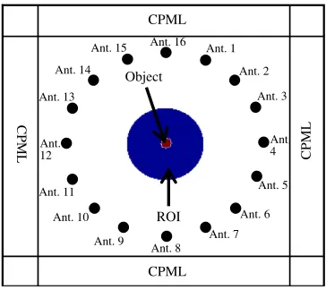
Figure 1. Configuration of the FD-FBTS in 2-D FDTD scheme.
The purpose of this technique is to resolve the shape, location and electric properties of any electromagnetic inverse scattering problem. The electric properties include the permittivity, permeability, electric conductivity and magnetic conductivity. Figure 1 shows a typical configuration of an active microwave tomography setup for FD-FBTS inverse scattering problem. The object is assumed to be embedded in a free space. The object is illuminated successively by M short pulsed waves generated by current sources sm(r, t) located at r = rtm(m = 1,2, . . . , M). The 16 antennas shown in Figure 1 will take turn to transmit a gaussian pulse towards the region of interest (ROI) one at a time while the remaining antennas will become the receivers.
The weighty challenge in solving inverse scattering problem is reconstructing the electric properties’ profile utilizing the knowledge of the transient field data measured at several observation points r=rnt(n= 1,2, . . . , N) for each illumination. For the initial condition, the currents are assumed to be generated at time t = 0 and there are no electromagnetic fields found before time t = 0. Hence, the total electromagnetic fields vm(r, t) for the mth current sourcesm(r, t) satisfy the following Maxwell’s equation:
Lvm =sm (13)
Under zero initial condition for
vm(r,0) = 0 (14)
whereL is the Partial Differential Equation operator of Maxwell’s equations.
To initialize the FD-FBTS procedure, an optimization problem is formulated in the form of cost functional Equation (4) to be minimized.
In FD-FBTS technique, the error is calculated with the difference between measured and calculated microwave scattering data in time domain at each antenna for every combination as mentioned in Equation (4). The gradient of the error functional with respect to p is calculated by using a forward Finite-Difference Time-Domain (FDTD) computation. Then, a corresponding adjoint FDTD computation is carried out by exploiting the residual received signals as equivalent sources which are reversed in time. In FD-FBTS, Dai Yuan conjugate gradient method is used for optimization technique to solve the inverse scattering problem.
4. RESULTS AND DISCUSSIONS
of the signal at the boundary of the FDTD lattice. The FD-FBTS algorithm was simulated up to 100 iterations utilizing 16 antennas to reconstruct the embedded object.
The size for the region of interest (ROI) is set to 80 mm in diameter while the size for the object is set to 10 mm in diameter. The electrical properties for the ROI and object are summarized in Table 1.
Table 1. Electrical properties of the region of interest and object.
εs ε∞ σs τ Region of Interest 10.00 7.00 0.15 7.00e-12
Object 21.57 6.14 0.31 7.00e-12
(a) (b) (c)
Figure 2. Original profiles of the model used (a) relative permittivity at infinite frequency, (b) static relative permittivity, (c) static conductivity.
(a) (b) (c)
(d) (e) (f)
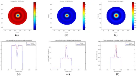
The foundation of this approach is formulated utilizing Debye equation as expressed in Equation (1). Figure 2 illustrates the original profiles of the circular model used in this work. Figure 3(a) shows the reconstructed relative permittivity at infinite frequency and indicating that the shape and size of the object is able to be detected and reconstructed for relative permittivity at infinite frequency. Figure 3(d) shows the cross-sectional view of the reconstruction Figure 3(a) at the axis x = 110 which is at the center point.
Figure 3(b) shows the reconstructed static relative permittivity in which the object’s shape and size are reconstructed. Figure 3(e) shows the cross-sectional view of the reconstruction Figure 3(b) at the axisx= 110 which is at the center point.
Figure 3(c) shows the reconstructed static conductivity in which the size and shape of the embedded object are able to be detected and reconstructed. Figure 3(f) shows the cross-sectional view of the reconstruction Figure 3(c) at the axis x= 110 which is at the center point.
The reconstruction of the three electrical properties have been analysed and the mean square error (MSE) are calculated respectively. The MSE of the reconstructed electrical properties are 0.0761, 0.6485 and 0.00019428 for relative permittivity at infinite frequency, static relative permittivity and static conductivity, respectively.
5. CONCLUSIONS
The iterative FD-FBTS algorithm can be used to resolve the dispersive electrical properties of an inverse scattering problem using broadband microwave signal in time domain. The shape and size of a simple embedded object are reconstructed in all three dispersive electrical properties.
ACKNOWLEDGMENT
This research was supported by Research Acculturation Collaborative Effort (RACE) grant scheme (RACE/c(3)/1332/2016(5)).
REFERENCES
1. Shea, J. D., P. Kosmas, S. C. Hagness, and B. D. van Veen, “Three-dimensional microwave imaging of realistic numerical breast phantoms via a multiple-frequency inverse scattering technique,”Med. Phys., Vol. 37, 4210–4226, 2010.
2. Hassan, M. and A. M. El-Shenawee, “Review of electromagnetic techniques for breast cancer detection,”IEEE Rev. Biomed. Eng., Vol. 4, 103–118, 2011.
3. Winters, D. W., J. D. Shea, P. Kosmas, B. D. van Veen, and S. C. Hagness, “Three-dimensional microwave breast imaging: Dispersive dielectric properties estimation using patient-specific basis functions,”IEEE Trans. Med. Imaging, Vol. 28, No. 7, 969–981, 2009.
4. Winters, D. W., E. J. Bond, B. D. van Veen, and S. C. Hagness, “Estimation of the frequency-dependent average dielectric properties of breast tissue using a time-domain inverse scattering technique,”IEEE Trans. Antennas Propag., Vol. 54, No. 11, 3517–3528, 2006.
5. Deng, Y. and X. Liu, “Electromagnetic imaging methods for nondestructive evaluation applications,” Sensors, Vol. 11, No. 12, Basel, Switzerland, 2011.
6. Pastorino, M., S. Caorsi, and A. Massa, “A global optimization technique for microwave nondestructive evaluation,” IEEE Transactions on Instrumentation and Measurement, Vol. 51, No. 4, 666–673, 2002.
7. Rufus, E. and Z. C. Alex, “Microwave imaging system for the detection of buried objects using UWB antenna — An experimental study,”PIERS Proceedings, 786–788, Kuala Lumpur, Malaysia, Mar. 27–30, 2012.
9. Xu, H., T. Li, and Y. Sun, “The application research of microwave imaging in nondestructive testing of concrete wall,”2006 6th World Congress on Intelligent Control and Automation, Vol. 1, 5157–5161, 2006.
10. Davis, S. K., E. J. Bond, X. Li, S. C. Hagness, and B. D. van Veen, “Microwave imaging via space-time beamforming for early detection of breast cancer: Beamformer design in the frequency domain,” Journal of Electromagnetic Waves and Applications, Vol. 17, No. 2, 357–381, 2003. 11. Guo, B., J. Li, H. Zmuda, and M. Sheplak, “Multifrequency microwave-induced thermal acoustic
imaging for breast cancer detection,”IEEE Trans. Biomed. Eng., Vol. 54, No. 11, 2000–2010, 2007. 12. Curtis, C. and E. Fear, “Beamforming in the frequency domain with applications to microwave breast imaging,” 2014 8th European Conference on Antennas and Propagation (EuCAP), 72–76, 2014.
13. Franchois, A. and C. Pichot, “Microwave imaging-complex permittivity reconstruction with a Levenberg-Marquardt method,”IEEE Trans. Antennas Propag., Vol. 45, No. 2, 203–215, 1997. 14. Caorsi, S., G. L. Gragnani, and M. Pastorino, “Two-dimensional microwave imaging by a numerical
inverse scattering solution,”IEEE Trans. Microw. Theory Tech., Vol. 38, No. 8, 981–989, 1990. 15. Rekanos, T. T. and T. D. Tsiboukis, “A combined finite element — Nonlinear conjugate gradient
spatial method for the reconstruction of unknown scatterer profiles,”IEEE Trans. Magn., Vol. 34, No. 5, 2829–2832, 1998.
16. Papadopoulos, T. G. and I. T. Rekanos, “Time-domain microwave imaging of inhomogeneous Debye dispersive scatterers,” IEEE Trans. Antennas Propag., Vol. 60, No. 2, 1197–1202, 2012.
17. Papadopoulos, T. G., T. I. Kosmanis, and I. T. Rekanos, “Microwave imaging of dispersive scatterers using vectorial lagrange multipliers,” PIERS Proceedings, 1926–1931, Prague, Jul. 6– 9, 2015.
18. Takenaka, T., H. J. H. Jia, and T. Tanaka, “An FDTD approach to the time-domain inverse scattering problem for na lossy cylindrical object,” 2000 Asia-Pacific Microw. Conf. Proc. (Cat. No. 00TH8522), Vol. 8, No. 2, 3–6, 2000.
19. Takenaka, T., H. Jia, and T. Tanaka, “Microwave imaging of electrical property distributions by a forward-backward time-stepping method,” Journal of Electromagnetic Waves and Applications, Vol. 14, No. 12, 1609–1626, 2000.
20. Ping, K. A. H., T. Moriyama, T. Takenaka, and T. Tanaka, “Two-dimensional Forward-Backward Time-Stepping approach for tumor detection in dispersive breast tissues,” 2009 Mediterrannean
Microwave Symposium (MMS), 1–4, 2009.
21. Johnson, J. E., T. Takenaka, K. Ping, S. Honda, and T. Tanaka, “Advances in the 3-D Forward-Backward Time-Stepping (FBTS) inverse scattering technique for breast cancer detection,” IEEE Trans. Biomed. Eng., Vol. 56, No. 9, 2232–2243, 2009.
22. Ng, S. W., K. A. H. Ping, L. S. Yee, W. Z. A. Wan Azlan, T. Moriyama, and T. Takenaka, “Reconstruction of extremely dense breast composition utilizing inverse scattering technique integrated with frequency-hopping approach,” ARPN J. Eng. Appl. Sci., Vol. 10, No. 18, 8479– 8484, 2015.
23. Yong, G., K. A. H. Ping, A. S. C. Chie, S. W. Ng, and T. Masri, “Preliminary study of forward-backward time-stepping technique with edge-preserving regularization for object detection applications,” 2015 International Conference on BioSignal Analysis, Processing and Systems (ICBAPS), 77–81, 2015.