Abstract—The authors present an analysis of conditions on the boundary between layers having varied electromagnetic properties. The research is performed using consistent theoretical derivation of analytical formulas, and the underlying problem is considered also in view of multiple boundaries including the effect of the propagation of electromagnetic waves with different instantaneous speeds. The paper comprises a theoretical analysis and references to the generated algorithms. The algorithms were assembled to enable simple evaluation of all components of the electromagnetic field in relation to the wave propagation speed in a heterogeneous environment. The proposed algorithms are compared by means of different numerical methods for the modelling of electromagnetic waves on the boundary between materials; moreover, the electromagnetic field components in common points of the model were also subject to comparison. When in conjunction with tools facilitating the analysis of material response to the source of a continuous signal, the algorithms constitute a supplementary instrument for the design of a layered material. Such design allows us to realize, for example, a recoilless plane, recoilless transition between different types of environment, and filters for both optical and radio frequencies.
1. INTRODUCTION
Inhomogeneities and regions with different parameters generally appear even in the cleanest materials. During the passage of an electromagnetic wave through a material, we can observe an amplitude decrease and wave phase shift. These phenomena are due to material characteristics, such as conductivity, permittivity, or permeability [1]. If a wave impinges on an inhomogeneity, there occurs a change in its propagation. The change manifests itself in two forms, namely in reflection and refraction. In addition to this process, polarisation and interference may appear in these waves [1–5].
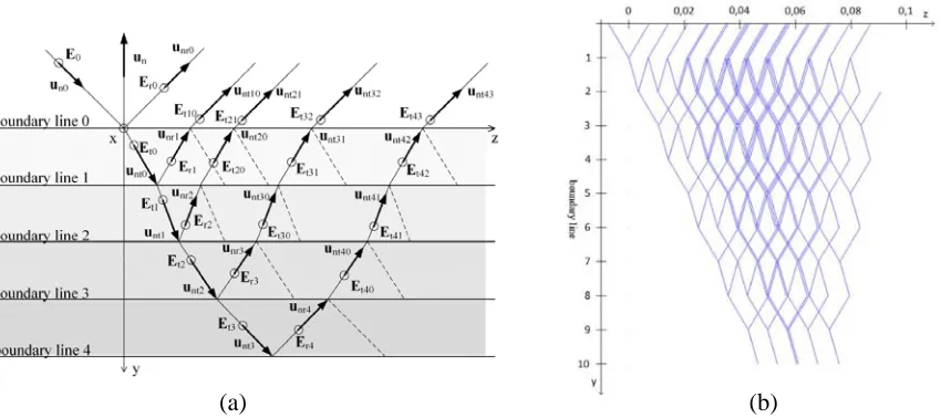
In the Matlab program, algorithms were created that simulate reflection and refraction in a lossy environment on the boundary between two dielectrics. The propagation of the waves is in accordance with Snell’s law for electromagnetic waves. This law can be applied in a wide range of cases, starting from the optical principles of reflection and refraction and ending with, for example, the complex phenomena of the interference and propagation of waves. Referring to Snell’s law, the reflection and refraction of electromagnetic waves is presented in Figure 1(a) and can be written as shown in [1]:
sinθ0
sinθ2
= k2
k1
=
jωμ2·(γ2+jωε2)
jωμ1·(γ1+jωε1)
, (1)
wherek is the wave number,γ the conductivity,ε the permittivity,μthe permeability, θ0 the angle of
incidence, and θ2 the angle of refraction. The interpretation of the Fresnel equations and Snell’s laws
is simple in the case of refraction on the boundary line between dielectrics. In the case of refraction in a lossy medium, the angle θ2 depends on the wave numbers k1 and k2, which are generally complex.
Received 29 April 2015, Accepted 25 June 2015, Scheduled 29 June 2015 * Corresponding author: Radim Kadlec ([email protected]).
(a) (b)
Figure 1. (a) Reflection and refraction of a TE wave [1]; (b) propagation of the constant phase and amplitude.
Thus, according to Formula (1), the angle θ2 lies within complex numbers. Although this condition
may appear uncommon, it is physically interpretable. In a lossy medium, planes of constant amplitude and phase propagate in different directions, and the transmission wave is not a plane wave.
The real part of the complex vector k describes the distribution of a wave in space, and simultaneously, it is perpendicular to the constant phase plane. The imaginary part of the same vector
kthen describes the damping of the wave and is perpendicular to the constant amplitude plane. If both the components of the complex vector k are parallel, the wave is classified as homogeneous; we denote it as inhomogeneous in all other cases.
Snell’s law (1) can be expressed in components [6]. The real component of the wave numberkuni
forms the angleϕwith the vector un, and the imaginary component of the wave numberkuni makes the angle Φ with the same vectorun. If the boundary conditions and the generalised Snell’s law (1) are valid, we also have
kuni=k(un·cosϕ+t·sinϕ) +i k(un·cosυ+t·sinυ). (2) After modification, we obtain the formula
kuni=unk·cosϕ+i k·cosυ+tk·sinϕ+i k·sinυ, (3)
which gives
k0·sinϕ0+i k0·sinυ0
=k2·sinϕ2+i k2·sinυ2
. (4)
According to Equation (4), the itemised Snell’s law in real variables is expressed as
k1 sinϕ1=k2 sinϕ2 (5)
k1sinυ1=k2sinυ2, (6)
wherek2 is the real component, forming the angleϕ2 with the perpendicular line at the boundary, and k2 is the imaginary component, making the angle υ2 with the perpendicular line at the boundary. It
follows from the formulas that υ= 0 orυ =π, as is obvious from Figure 1(b).
An electromagnetic wave exhibits an electric and a magnetic field intensity. The electric and magnetic components of the incident wave according to Figure 1(a) follow from the related formula specified in [1]:
Ei =E0e−jk1un0·r, Hi=
un0×Ei Zv1
, (7)
whereE0 is the amplitude of the electric field intensity on the boundary line, ris the positional vector, and un0 is the unit vector of the propagation direction. Zv is wave impedance:
Zv =
jωμ
Zv1 Zv1 Zv2
The calculation of the reflection coefficientρE and the transmission factorτE is performed, via utilising the wave impedance Zv, as follows:
ρE = E1
E0
= Zv2cosθ1−Zv1cosθ2
Zv2cosθ1+Zv1cosθ2
, τE= E2 E0
= 2Zv2cosθ1
Zv2cosθ1+Zv1cosθ2
. (12)
For a more suitable analysis of the dependence of the reflected and refracted waves on the parameters of the medium, we can advantageously use the formula
Er=
μ2k1cosθ0−μ1
k22−k21sin2θ0
μ2k1cosθ0+μ1
k22−k21sin2θ0
E0·e−jk1un1×r,
Et= 2μ2k1cosθ0
μ2k1cosθ0+μ1
k2
2 −k21sin2θ0
E0·e−jk2un2×r.
(13)
The formulas to derive the magnetic component are usually written as
Hr= un1×Er
Zv1
, Ht= un2×Et
Zv2
. (14)
In some cases, it can be more effective to directly utilise the basic variables. Thus, if the Poynting vector is applied, we have the following formula:
Hr=−
µ2
µ1k1cosθ0−
k2
2−k21sin2θ0 μ2cosθ0+µ1k1
k22−k12sin2θ0 E0
ω ·e
−jk1un1·r,
Ht=− 2k2cosθ0
μ2cosθ0+µ1k1
k22−k12sin2θ0 E0
ω ·e
−j k2un2·r.
(15)
2. OBLIQUE WAVE INCIDENCE ON A LAYERED MEDIUM
For a layered heterogeneous medium [7], we derive the algorithm according to Figure 2(a). The reflection of the electric component of the electromagnetic field intensity on the first layer is solved via the equations
Er0 =Ei0ρE0·e−jk1unr0×r0, Et0=Ei0τE0·e−jk2unt0×r0. (16)
The reflection and refraction of the electric component of the electromagnetic field intensity on an arbitrary layer is expressed as
(a) (b)
Figure 2. Reflection and refraction of the electric component of an electromagnetic wave on a layered medium: (a) layout; (b) Matlab for 2000 cycles.
whereErl aEtl are the reflected and refracted electromagnetic waves on the boundary linel (l= 1,. . ., max) according to Figure 2(a), Eil is the maximum value of the electric field intensity on the boundary line l,ρEl and τEl are the reflection coefficient and transmission factor on the boundary linel,kl is the wave number of the layer, rl is the wave incidence positional vector on the boundary line l, and untl
and unrl are the unit vectors of the propagation direction.
The magnetic component, or intensity of the magnetic field for the reflection on the first layer, leads to the formulas
Hr0 =−Hi0ρH0·e−j k1unr0×r0, Ht0=−Hi0τH0·e−jk2unt0×r0. (18)
The reflection and refraction of the magnetic field intensity on several layers is expressed as
Hrl=−HilρHl·e−jk(l+1)unrl×rl, Htl=−HilτHl·e−jk(l+2)untl×rl, (19)
where Hrl and Htl are the reflection and refraction magnetic components of the EMG wave at the boundaryl. The other quantities are denoted similarly to Equation (17).
A Matlab-based analysis using Equations (1)–(19) was carried out to investigate the layered structure. An EMG wave having the frequency of 1.5 GHz impinges on the boundary of the material under the angleθ0, where it reflects and refracts. The wave passes through the material, which comprises
ten layers of an identical thickness, namely d = 20 mm (Figure 3). The parameters of material 1 are as follows: εr1 = 1, μr1 = 1, and γ1 = 1·10−9S/m. The parameters corresponding to material 2 are εr2 = 4, μr2 = 0.999991, and γ2 = 1·10−9S/m. In the other layers, the material parameters vary
regularly. The surrounding medium of the layered sample is defined by the parametersεr0= 1,μr0 = 1
andγ0= 1·10−9S/m. During the solution and analysis of the FEM-based model, the high permittivity
of a medium resulted in an unfavourable division of the discretised mesh elements with respect to the length of the propagating wave. Considering this fact, we then selected the material parameters; however, these are suitable only for testing purposes and cannot be practically applied. The geometry of the electromagnetic wave propagation inside the medium is represented via the proposed analysis as shown in Figure 2(b).
Figure 3. Geometrical model and dimensions of the wave incidence on a layered medium.
Figure 4. Oblique incidence on a layered medium ford=λ·100 andt=T (f = 700 THz).
whereλrepresents the wavelength of the wave emitted by the source; this wave is generated as a single pulse, a single period. The distribution of the modules of the electric field intensity Eon the surface of the material is obvious from the behaviour of the propagation of the electromagnetic waves inside the layered material indicated in Figure 1(b).
3. FEM-BASED MODEL OF A LAYERED MEDIUM
In order to verify the properties of the described analytical analysis, we performed an equivalent comparative evaluation based on the FEM; this analysis exhibited the same parameters as the previous model. As the mathematical expression, we applied the extended wave equation for a lossy environment:
∇2u+f∂u ∂t +g
∂2u
∂t2 −fc(x, y, z, t) = 0, ∀g(x, y, z)= 0, ∀f(x, y, z)= 0, in Ω, (20)
(a) (b)
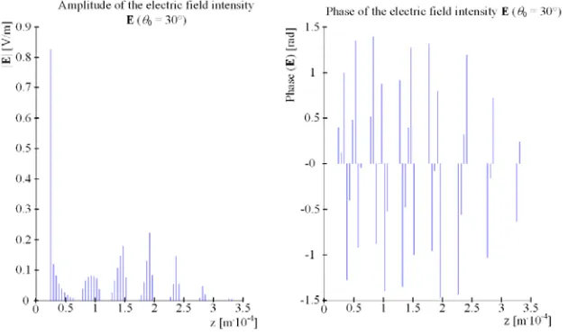
Figure 5. Distribution of the electric field intensity E: (a) the amplitude, and (b) the phase for
θ0= 40◦.
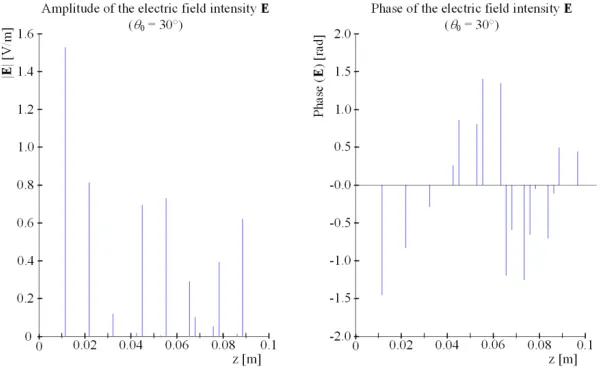
Figure 6. Intensity of the electric component of the TE wave on a layered medium at the angle θ0 =
30◦.
layer plane (Figure 3). The FEM-based solution in ANSYS limits the resulting values and manifests itself through the non-continuous distribution of values within the model.
4. COMPARISON OF THE MODEL RESULTS
Direct comparison of the results of the different analyses [9] obtained via the applied methods can be performed only with substantial difficulty. The results of the designed analytical parameters represent the waveform of the material response to the wave emitted by the pulse source, and changes of the maximum value of the electric field intensity are evaluated. The FEM is employed to represent the behaviour of the electric field intensity inside the examined layered medium; this pattern constitutes the response to the EMG waves from the continuous source.
For this reason, we designed algorithms to evaluate the selected time intervals in the ray-tracing model. The evaluation of the module of the electric field intensity E on the surface of the material at these time intervals [10] is indicated in Figure 6.
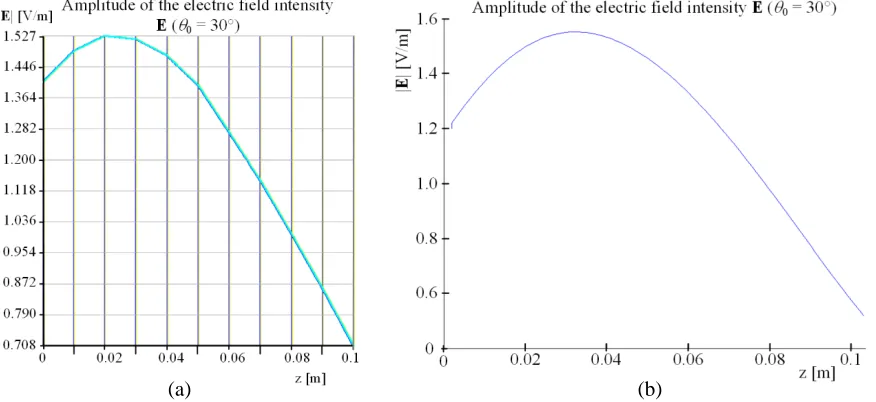
(a) (b)
Figure 7. Distribution of the module of the electric field intensity E for θ0 = 30◦ in the plane of
the wave incidence on the surface of the material: (a) the behaviour obtained from ANSYS; (b) the amplitude achievable with the designed algorithms.
according to the formula
f(x) =|E| 1 σ√2πe
−(x−2σΔ2x)2, (21)
where Δx is the mean value of distribution, σ is the scattering parameter, and |E| is the module of the electric field intensity. The scattering parameter was selected to be σ = 1, and the mean value of distribution was set as Δx = 0. The Gaussian function merely approximates the ray tracing-based evaluation to the FEM, which comprises wave propagation. The radiation source generates a continuous electromagnetic wave. After approximating with the Gaussian function, we obtain the courses in Figure 7(b) from the patterns shown above (Figure 6). A suitably chosen time interval of the approximated response of the medium embodied in the discrete maximum values of the electromagnetic field intensity facilitates comparison with the evaluated continuous instantaneous values acquired via the FEM from Figure 7(a). The diagrams show that the results of the analyses are comparable; however, it is important to note that the module of the electric field intensityEevaluated from the ANSYS-based analyses is not represented in the range between 0 and the maximum.
The EMAG module of ANSYS is not applicable as a tool convenient for the evaluation of either the pulse process or the maximum values of an electromagnetic wave in a heterogeneous environment. This drawback stems from the fact that the module is characterised by multiple interferences and various wave propagation velocities, and therefore the behaviour of the phase of the electromagnetic field intensity is not uniform. Moreover, if the parameters described herein are set, the number of the discretisation mesh divisions in the ANSYS-based model will be unfavourable with respect to the wavelength of the propagating wave. For comparison purposes, however, this negative effect is still acceptable. Consequently, the resulting values (and thus also the comparison possibilities) are restricted.
5. CONCLUSIONS
It is obvious from the above-shown patterns that the designed algorithms are applicable to a large number of effects characterising the propagation of electromagnetic waves; simultaneously, the algorithms also enable us to define the parameters of both the wave sources and the environment through which the waves propagate. The verified methods facilitate the use of point, planar and pulse sources as well as those generating a continuous EMG wave. The response of the medium can be evaluated as a whole, and it is also possible to select certain points in the geometry or specific time instants. A limitation (but also an advantage for some cases) seems to consist in the possibility of representing the modules and phases instead of the instantanteous values. Principally, we can note that although algorithms based on ray tracing do not comprise the wave character of the propagation of an electromagnetic wave, they represent more illustratively the behaviour of a propagating wave in space and time. This fact may be beneficial for the quantitative approach to analysing the details of the model.
The main obstacle to direct comparison of the described approaches is the dissimilarity of the principles defining the individual analyses. Numerical modelling performed via the wave equation and ANSYS produces a continuous source of electromagnetic waves. Interference effects between the reflected and refracted waves arise on the boundary between the layers. Furthermore, the interference process is also accompanied by the time-delayed waves from the source and by interface reflections [11, 12]. Conversely, however, the designed analytical analysis does not comprise all types of interferences, and it evaluates several time-delayed responses to an EMG wave from the pulse source. The analytical solution and its algorithms process the time-varying phenomena of the pulsed source. This analytical solution includes the time-dependent propagation of electromagnetic waves in a heterogeneous medium and evaluates the distribution of the electromagnetic field on the surfaces of the boundaries at certain moments of time. A complex form of the angle of reflection and refraction is considered in the case of the analytical approach, which allows accurate determination of the size of the intensity of the reflected and refracted waves. In order to determine the direction of the constant phase propagation in a lossy medium, we consider only real parts of the wave number, which must be evaluated separately.
The results obtained from indirect comparison point to general agreement between the analyses. The FEM-based solution in ANSYS is restricted to the spatial distribution of the quantities with distributed parameters. This approach, despite being very robust in the time domain, appears to be inconvenient for the solution of multilayers due to the manner in which the mesh of elements is divided. In FEM-based numerical models, the number of divisions of the discretised mesh assuming the wavelength of the propagating wave can be determined only with difficulty, and a large model is almost unsolvable by common means. Importantly, this drawback is eliminable via the proposed method.
Advantageously, the presented analysis allows us to acquire an accurate solution of the response of an electromagnetic field to very short pulses and transient or continuous exciting electromagnetic sources. In connection with tools facilitating the analysis of the response of the material to a source of a continuous signal, the proposed algorithms constitute a supplementary instrument to enable the design of a layered medium.
The author has theoretically derived the analytical expressions to evaluate both the incidence of an EMG wave upon a boundary between layers with different electromagnetic properties and the behaviour of an electromagnetic wave on/in multilayered structures. The analytical relations have been applied in conjunction with ray-tracing. Finally, the derived formulas were compared with similar, commonly used numerical models.
ACKNOWLEDGMENT
Research described in this paper was financed by the Czech Science Foundation under grant no. GA15-08803S, a project of the BUT science fund, no. FEKT-S-14-2545.
REFERENCES
summarizing approach,”Proceedings of the IEEE, Vol. 72, No. 5, 595–611, 1984, ISSN: 0018-9219. 8. Kadlec, R., “Analysis of an electromagnetic wave on the boundary between heterogeneous materials,” 84, Doc. Ing. Eva Kroutilov´a, Ph.D., Supervisor, Faculty of Electrical Engineering and Communication, Brno University of technology, Brno, 2014.
9. Novitsky, A. V., S. V. Zhukovsky, L. M. Barkovsky, and A. V. Lavrinenko, “Field approach in the transformation optics concept,” Progress In Electromagnetics Research, Vol. 129, 485–515, 2012. 10. Myˇska, R. and P. Drexler, “The development of methods for estimation of time differences of arrival
of pulse signals,”PIERS Proceedings, 709–713, Kuala Lumpur, Malaysia, Mar. 27–30, 2012. 11. Drexler, P. and R. Kub´asek, “Pulsed magnetic field fiber optic sensor based on orthoconjugate
retroreflector,”Proceedings of SCS 2009 International Conference on Signals, Circuits and Systems, 52–57, Tunisia, 2009, ISBN: 978-1-4244-4398-7.
![Figure 1. (a) Reflection and refraction of a TE wave [1]; (b) propagation of the constant phase andamplitude.](https://thumb-us.123doks.com/thumbv2/123dok_us/1989063.1263118/2.612.95.530.69.272/figure-reection-refraction-wave-propagation-constant-phase-andamplitude.webp)