INFLATION AND STOCK MARKET VOLATILITY IN KENYA
BENARD GIBET
K102/12092/2009
RESEARCH PROJECT SUBMITED TO THE DEPARTMENT OF STATISTICS AND ECONOMETRICS IN PARTIAL FULFILMENT OF THE REQUIREMENT FOR AWARD OF MASTER OF ECONOMICS (ECONOMETRICS) DEGREE OF
KENYATTA UNIVERSITY
i DECLARATION
This research project is my original work and has not been presented for a degree award in
any university.
Signature ………..Date………
BENARD GIBET
(Bachelor of Arts)
K102/12092/2009
This study is presented with my approval as supervisor
Signature ………..Date………
DR. JULIUS KORIR
Department of Economic Theory
ii DEDICATION
This study is dedicated to my father Daniel Kilele my mother Mary Kilele, my beloved wife
iii ACKNOWLEDGEMENT
I am greatly indebted to the almighty God for giving me knowledge and good health. I am
also grateful to my supervisor Dr. Julius Korir for the advice and the time accorded
throughout the duration of the project. Thanks to all the lecturers at the School of
Economics, Kenyatta University.
I also owe a lot of thanks to my parents Daniel Kilele and Mary Kilele. Special thanks to
my colleague Salome Thinguri for the encouragement in the entire period of study. To my
wife Faith Chebor, brothers and sisters thank you for the encouragement and emotional
support throughout my study.
iv TABLE OF CONTENTS
DECLARATION ...i
DEDICATION ... ii
ACKNOWLEDGEMENT ... iii
TABLE OF CONTENTS ... iv
OPERATIONAL DEFINITION OF TERMS... vi
ABBREVIATIONS ... vii
ABSTRACT ... viii
CHAPTER ONE ...1
INTRODUCTION ...1
1.1 Background ...1
1.2 The Stock Market in Kenya ...4
1.3 Inflation in Kenya...6
1.4 Statement of the Problem ...7
1.5 Research questions ...8
1.6 Objectives ...8
1.6.1 General objective ... 8
1.6.2 Specific objectives... 8
1.7 Significance of the study...8
1.8 Scope and limitation ...9
1.9 Organization of the study ...9
CHAPTER TWO ... 10
LITERATUREREVIEW ... 10
2.1 Introduction to Literature ... 10
2.2 Theoretical Literature ... 10
2.2.1 Fisher Hypothesis ... 10
2.2.2 Proxy Hypothesis ... 10
2.3 Empirical Literature... 12
2.4 Overview of Literature ... 24
CHAPTER THREE ... 27
RESEARCH METHODOLOGY ... 27
3.1. Introduction ... 27
v
3.3. Empirical model ... 27
3.4. Definition and measurement of variables ... 30
3.5. Data types and sources ... 32
3.6. Data analysis ... 32
CHAPTER FOUR ... 33
RESULTS AND DISCUSSIONS ... 33
4.1 Introduction ... 33
4.2 Summary statistics ... 33
4.3 Diagnostic Tests ... 33
4.4 Results of Bounds Testing Approach to Cointegration... 38
4.5 Co-integration Results and Estimated Long run-coefficients using ARDL approach ... 39
4.6 Cointegration Analysis... 40
4.7 Cointegration Results ... 42
4.8 Error Correction Model results ... 43
CHAPTER FIVE... 45
SUMMARY, CONCLUSION AND IMPLICATIONS ... 45
5.1 Summary ... 45
5.2 Conclusion ... 46
5.3 Policy Implications ... 47
5.4 Suggestions for Further Research ... 47
Bibliography ... 48
Appendix ... 54
Table A1: Result for VAR Lag Order Selection Criteria ... 54
Table A2: Results on Serial Correlation ... 60
Table A3: Stability Test ... 67
Table A4: Johansen Cointegration Test... 72
Table A5: Vector Error Correction Estimates... 81
vi OPERATIONAL DEFINITION OF TERMS
Asymmetry this is the downward movements in the stock market that is followed by higher volatilities, than the upward movements of the same size.
Increased Supply of shares this is achieved through initial public offers and privatization of state owned enterprises
Price Discovery is the process of determining the price of a financial instrument in a stock market
Stock market volatility refers to variations in the stock price over time.
Stable price levels this is low inflation
Stock market returns is the log of sector price earnings ratio
vii ABBREVIATIONS
AR Autoregressive
ARDL Autoregressive Distributed Lag Model
Cap Chapter
CMA Capital Markets Authority
CPI Consumer Price Index
EGARCH Exponential Generalized Autoregressive Conditional Heteroscedastic
GARCH Generalized Autoregressive Conditional Heteroscedastic
IGARCH Integrated Generalized Autoregressive Conditional Heteroscedastic
ISE Istanbul Stock Exchange
JSE Jamaica Stock Exchange
LA-VAR Lag-Augmented Vector Auto-regression
NSE Nairobi Securities Exchange
OECD Organization for Economic Co-operation and Development
OLS Ordinary Least Squares
QGARCH Quadratic Generalized Autoregressive Conditional Heteroscedastic
SADC South African Development Community
U.K United Kingdom
USA United States of America
UVAR Unrestricted Vector Auto-regression
VAR Vector Auto-regression
viii ABSTRACT
1
CHAPTER ONE INTRODUCTION
1.1 Background
The relationship between the stock market and macroeconomic forces has been widely
studied. The extensive literature on relationship between stock market volatility and
inflation in the developing and emerging markets mainly cover the linkages between the
equity prices and the macroeconomic variables such as inflation, interest rate and exchange
rate. The studies have discovered significant effects of macroeconomic variables on stock
returns and indicated that stock prices are sensitive to macroeconomic variables. However,
very few studies have been done on the interaction between inflation and stock market
volatility especially on the sector-specific indices and price-earnings ratio (Diaz and Jareno
(2005; Grouard, Levy and Lubochinsky, 2003).
The impact of macroeconomic variables on the stock market volatility varies when sectoral
level data are used. Evidence shows that some sectors are more volatile than others. (The
studies found technology and telecommunications sector, financial, real estate services, and
oil and energy sectors less sensitive to inflation. These studies show that sectors respond
differently to inflation across firms and sectors of the stock exchange especially the
difference in the transfer of inflation shocks to the prices of their products particularly in
terms of magnitude and direction (Boudoukh, Richard and Whitelaw (1994); Geyser and
Lowies (2001); Grouard et al. (2003); Jareno (2005); Junhua (2008); Diaz and Jareno
(2009); and Chinzara (2011). Thus, the ability to transfer inflation shocks is affected by
2
volatility is affected by money supply and exchange rates, industrial production, oil prices
and interest rates.
Investors and traders of financial market when making decisions rely on their ability to
assess market risk and the likely profitability of the financial assets and maximize the
returns from their investments. This has led to various researches being undertaken to
analyze the forces that determine the equilibrium market volatility. The major connection
between inflation and stock market volatility has generated interest on how to evaluate
financial risk. This has led to various models being developed to model volatility and
measure volatility, the models developed aimed to assist the portfolio manager and risk
manager to predict volatility. The risk manager, an investor and portfolio manager in
mitigating their risk must have prior knowledge of the future performance of their
portfolio. They can appropriately manage their portfolios if they are able to use inflation as
a reliable indicator for where the stock market is heading.
Some explanations state that the relationship between stock return and inflation is a
reflector of real activity in the economy. Researchers have documented volatility of stock
markets acting as the most important factor in the economic growth of an economy (Fama
(1981); Wang (2011). Additionally, literature indicates that increased price volatility can in
the long run impact on the ability of listed firms in raising capital.
Volatility breeds uncertainty, which impair effective performance of the financial sector as
well as the entire economy at large. An unexpected increase in volatility today leads to the
upward revision of future expected volatility and risk premium which further leads to
discounting of future expected cash flows (assuming cash flows remains the same) at an
increased rate which results in lower stock prices or negative returns today. Stock return
3
more often is perceived by investors and other agents as a measure of risk. On their part,
policymakers and rational investors use market estimate of volatility as a tool to measure
the vulnerability of the stock market.
According to Aliyu (2010), there is a strong asymmetric relationship exists between stock
returns and stock returns volatility, and stock price volatility is higher when stock price
decreases than when stock price increases. Further researches examining volatility have
been done on the relationship between inflation and stock exchange volatility. Schwert
(1989) attempts to relate the changes in stock market volatility to macroeconomic factors;
inflation, industrial production and money supply. Schwert (1989) documented inflation
and real output had weak predictive power for the stock market volatility. Some studies
have found positive relationship between inflation and stock market returns (Engsted and
Tanggaard (2000); Anokye and Tweneboah (2008) while others have documented negative
relationship between inflation and stock market (Jaffe and Mandelker, 1976); Omran and
Pointman, 2001).
The impact of inflation on industry performance can be classified into three areas: the
supply side (production inputs), the demand side (consumption behavior), and the financing
cost of both the supply and the demand (cost of money). The impacts of inflation on
industry profitability tend to differ across industries due to different pricing power, market
dynamics, and financial conditions. Consequently, the timing of the stock market reaction
to the variations of inflation provides a good opportunity for investors to develop industry
rotation strategies to exploit this relationship. Junhua (2008) investigated the interaction
between global inflation and global industries and noted that sensitivities to inflation vary
significantly across industries and tend to be higher for noncyclical industries than those of
4
and Tobacco, all of which provide economic “necessities”, and therefore are, for the most
part, considered “recession proof”. In contrast, industries involved in the manufacture of
durable goods, such as Electrical Equipment, Automobiles, and Household Durables, are
severely impacted by economic downturns.
Despite the significance of volatility issue in decision making by investors on which sector
or firm to invest in there is little research that has so far been done to find how inflation rate
affects the sectors in the stock market (Chinzara, 2011; Geyser and Lowies, 2001). This
study filled this gap by investigating the relationship between inflation and return on the
different sectors listed on NSE.
1.2 The Stock Market in Kenya
Dealing in shares in Kenya began in 1920’s through Nairobi Stock Exchange. In 1951 an
estate agent Francis Drummond established the first professional stock broking firm in
Kenya. In 1954 the Nairobi Stock Exchange was constituted as a voluntary association of
stockbrokers and registered in 1991 as a limited company. NSE was responsible at the time
for regulating and developing the trading activities in the Stock Market, Ngugi (2003).
Development of the stock market involved changes in the institutional framework and
policy environment. The evolution indicated a graduation n from a non-formal market to a
formal organization without regulatory body. Thereafter the Capital Market Authority
(CMA) was established in the year 1989 through an Act of Parliament (Cap 485A) Laws of
Kenya and amended in the year 2000. In the new Act, CMA was mandated to promote,
regulate and facilitate development of an orderly, fair and efficient capital markets in
5
.
Figure 1.1: NSE 20 Share Index trends in Kenya
Source: Data used from Nairobi Securities Exchange 1996-2015
Figure 1.1 shows that there was downward trend in the stock market index from the year
1996 to the year 2002 before it began to rise. The upward trend continued to the year
2006 and reached its peak in January 2007. The lowest level ever reached by the stock
exchange was in March 2009 where the NSE 20 share index was at 2,360. The index
was relatively stable in the year 2007 and a decline began in the year 2008 until 2009
when it began to rise again.
In the month of November 2012 the number of listed companies stood at 55. Currently
the stock market has three segments namely Main Investment Market segment, the
Alternative Investment Market segment and the Fixed Income Securities Market
segments. In addition the NSE has ten sectors namely the agricultural, automobiles and
accessories, the banking, commercial and services, construction and allied, energy and
petroleum, insurance, investment, manufacturing and allied, telecommunication and
technology sectors. The Nairobi 20 share index was constructed to provide investors
6
capital and industry segments of the Kenyan market. The NSE 20 share index, in its
calculation, has companies with the largest 20 securities in market capitalization, issued
dividends and profitability. Another index was later added the Nairobi all share index
which presents the performance of all companies in the Securities Exchange.
The main functions of stock market are price discovery and provision of liquidity to
corporate by providing companies with a way of issuing shares through initial public
offering. The stock market performs a vital role in promoting economic growth and is an
avenue for investment. Government and corporate companies use the stock market for
raising capital for development projects.
1.3 Inflation in Kenya
In the study of stock market volatility in Kenya, it is important to track the levels of
inflation. The tracking helps in determining the impact of inflation on the stock market
volatility.
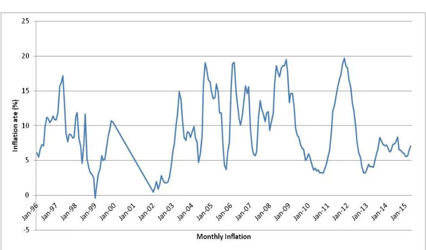
Figure 1.2 Monthly Inflation rate
7
From Figure 1.2 inflation has been varying between a high of 18.96 percent in September
2004 and a low of -0.44 percent in the month of January 1999. Inflation rate in Kenya has
been fluctuating across the period and has not been stable. In Figure 1.2 the effect of
inflation on stock market is expected to be the largest in the month of September 2004 and
the lowest in the month of January 1999.
1.4 Statement of the Problem
Relationship between the stock market and macroeconomic factors has been widely
studied. The extensive literature on relationship between stock market volatility and
inflation in the developing and emerging markets mainly cover the linkages between the
equity prices and the macroeconomic variables such as inflation, interest rate and exchange
rate. However, the impact of macroeconomic variables on the stock market volatility varies
when sectoral level data are used. Thus, the ability to transfer inflation shocks in to market
return or index is affected by how sensitive each sector is to inflation. This
notwithstanding, available literature provide evidence of mixed results of effects of
inflation on stock return volatility with some studies indicating that there are sectors which
react positively to inflation while others react negatively to inflation (Chinzara, 2011;
Grouard et al, 2003; Maysami, Howe and Hamzah, 2004).
In Kenya, both inflation and stock returns exhibit volatility. Inflation is shown to be
relatively more volatile than the stock market index. The emerging issue is whether or not
the inflation shocks affects the stock return volatility. Additionally, in view of the
mixed results, it is not clear as to what the effect is of inflation on market returns. Further,
its effects on different sectors also need to be examined. This is because investors and
portfolio managers need such evidence to guide portfolio investment decisions. The
8 sectoral and macro level.
1.5 Research questions
(i) What is the effect of inflation on stock market returns?
(ii) What are the effects of inflation on different sectors of the stock market in Kenya?
1.6 Objectives
1.6.1 General objective
In line with the research questions, the general objective of the study was to establish the
effect of inflation on stock market returns in Kenya.
1.6.2 Specific objectives
(i) To investigate the effect of inflation on the entire stock market returns.
(ii) To determine the effects of inflation on the different sectors in the stock market in
Kenya.
1.7 Significance of the study
The research is important to the policy makers, investors and the general public. The
research is important to the investors as it affects the stock pricing and risk decision
making. The results are important to policy makers to know determinants of stock market
volatility and the spill-over effects. The policy makers use the stock market condition as a
leading indicator of future macroeconomic condition and the results of the study may be
used to better control the direction and stability of the economy and identify critical factors
that drive market volatility. The investors may improve their portfolio performance in
selecting sectors that have positive returns during inflation. From a policy perspective, the
conclusions may provide useful insights for the formulation and implementation of fiscal
9 of stock market.
1.8 Scope and limitation
The scope of this study was limited to stock market data and inflation rate between 2006:9
to 2014:12. The price earnings ratio from 2006:1-2014:12. The study examined the effect
of inflation on the sectors of the stock market in Kenya.
1.9 Organization of the study
The remaining part of this study is organized as follows; chapter two a review of literature
on the effect of inflation on stock market while chapter three develops the methodology of
the study, chapter four presents the results and the interpretations and chapter five
10
CHAPTER TWO
LITERATUREREVIEW
2.1 Introduction to Literature
The chapter reviews both the theoretical literature on stock market and inflation and the
empirical literature on stock market and inflation.
2.2 Theoretical Literature 2.2.1 Fisher Hypothesis
Fisher theory (1930) postulates that the real rates of returns on common stocks do not
depend on inflation. Fisher indicates that stocks should be independent of inflation and
theoretically, stock returns should be positively related to the expected economic activity.
This implies that the investors are compensated for the increase in inflation level, through
increases in nominal stock returns thus real returns not being affected. The Fisher further
states that, in response to a change in the money supply, the nominal interest rate changes
in tandem with changes in the inflation rate in the long run. For example, if monetary
policy were to cause inflation to increase by 5 percentage points, the nominal interest rate
in the economy would eventually also increase by 5 percentage points.
2.2.2 Proxy Hypothesis
Fama (1981), developed proxy hypothesis that attempted to explain the anomalous negative
behavior that exists between the stock return and inflation. Fama’s argument was that the
negative relations between inflation and stock return was proxying for positive relations
between stock returns and real variables. The author argued the positive relationship
between the stock returns and real activity combines with the negative relationship between
inflation and real activity to induce the spurious negative relationship between the stock
11
return-inflation disappears when both real variables and measures of expected and
unexpected inflation are used to explain the stock returns.
Danthine and Donalson (1986), Stulz (1986), Boyle (1990) and Marshal (1992), predict
that stocks may fail to offer a hedge against inflation, especially when inflations is due to
non-monetary factors. The money enters into these models as an asset that provides
transactions services and whose value is determined simultaneously with other assets,
including stocks. Expectations of higher inflation reduce wealth by reducing the purchasing
power of money balances carried forward through time. This, in turn reduces expected real
returns on stock.
Danthine and Donaldson (1986) further argue that stocks provide protection against a
purely monetary inflation but fail to hedge against inflation arising from real output shocks.
Stulz (1986) predicts that real stock returns are adversely affected by expectations of higher
inflation arising from the monetary sector. However, the impact of an increase in expected
inflation on stock returns will be greater when the source of these expectations is due to a
worsening of the investment opportunity set rather than an increase in money growth.
Marshall (1992) predicts negative correlations between expected asset returns and expected
inflation, and that the association will be more strongly negative when inflation arises from
fluctuations in real economic activity than from the monetary sector.
Lee (1989), Giovannini and Labadie (1991) employ stochastic general equilibrium models
to explore the stock returns-inflation relationship. In these models, money demand arises
through a cash-in-advance constraint. Using simulation results from a four-variable VAR,
Lee (1989) finds negative cross-correlations between real stock returns and inflation.
12 hedge against inflation in the post-war time period.
2.3 Empirical Literature
Research studies have been conducted to determine the effects of inflation on aggregate
stock market. Most studies reveals inflation had negative effect on stock return. Fisher
Theory states that equities are a hedge against the increase of price level due to the fact that
they represent a claim to real assets and, hence, the real change on the price of the equities
should not be affected i.e. earnings should be consistent with the inflation rate, and
therefore the real value of the stock market should remain unaltered in the long-run.
However, Fama (1981) found a negative relationship between stock returns and stated that
the negative association found between stock returns and inflation is the result of two
underlying relationships between stock returns and expected economic activity; and
expected economic activity and inflation. Expectation of higher future dividend account for
a positive relationship between stock returns and inflation while money demand effects
account for a negative relationship between expected activity and inflation. This argument
is certainly plausible and is supported by compelling empirical evidence. However,
something of a puzzle still remains in Fama's (1981) empirical results. Various measures of
real activity did not, by themselves, entirely eliminate the negative inflation and stock
returns relation. The main aim of the section is to review empirical literature relating to
inflation and stock market.
Jaffe and Mandelker (1976) using data from New York Stock Exchange in the USA
measured return to the market as a whole using the Lawrence Fisher Index and consumer
price index as the measure of price level. The dependant variable is the market return while
the independent variable is the consumer price index while using simple regression model
13
indicated a negative relationship between inflation and stock market while using annual
data the inflation rate had a positive coefficient which suggested that stock market is a
partial hedge against inflation. The study in general found a negative relationship between
inflation and stock returns in the short run. In the long run the relationship was positive
between inflation and stock returns.
Lee (1992) using multivariate VAR approach investigated the causal relations and dynamic
interactions among asset returns, real activity and inflation in the U.S.A. The study was a
criticism on a study done by Geske and Roll’s (1983) and Ram and Spencer’s (1983), the
studies were on a bivariate causal test and believed that the result may not lead to valid
causal relations. The study used monthly data for real stock returns, real interest rates,
growth in industrial production and the rate of inflation. Based on cross correlations
between the period January 1947 and December 1987 the results indicated that there was
no causal link between stock returns and money supply growth hence no causal relationship
between inflation and both nominal and real stock returns.
Boudoukh and Richardson (1993) examined the long run relationship between stock returns
and inflation. The study was an extension of previous studies that had dwelt more on
shorter periods of between one year and less. The study was to fill the gap for the long run
relationship since the Fisher model is expected to hold over longer horizons. Inflation was
the independent variable in the study influencing the stock returns while using annual data
on inflation, stock returns and short term and long term interest rates from 1890-1990 from
USA and UK. The study looked at contemporaneous relationship between stock returns and
inflation using regression analysis. The results of the study indicated evidence that long
14
inflation. The one year stock returns were regressed on one year inflation while the five
year (long-horizon) stock returns was regressed on five year inflation. The regression
coefficient for the long horizon was positive, this showed that the stock returns and
inflation moved together in the long run. The results support the view that stocks provide
compensation for movements in inflation in the long run.
Using regression model Adrangi, Chatrah and Sanvincente (2000) studied the association
between inflation, output and stock prices in Brazil. In the study inflation was the
independent variable influencing both the output and the stock prices. Using the Johansen
and Juselius cointegration tests, the study observed a long-run equilibrium between
monthly stock prices, general price levels and the real economic activity. The findings of
the study indicated that real stock returns were not related to expected inflation. The study
concluded that the negative relationship between inflation rates and real stock returns
stemmed from the unexpected component of the inflation rate. The real stock return and
activity for Brazil had a positive relationship, in addition the study reports a negative
relationship between inflation and real activity.
Engsted and Tanggaard (2000) analyzed the relationship between asset returns as
dependent variable and inflation as independent at short and long horizons. The authors
criticized the study by Boudoukh and Richardson (1993) in that the approach of looking
over longer horizons, may cause time over-lap in data and requires a correction for the
estimated matrix. The authors noted that these corrections are unreliable especially when
the horizon is large. The study was a proposal for an alternative model to analyze the
relationship between more than two periods for asset returns and inflation. The study
measured multi-period expected returns and inflation from a VAR model involving one-
15
stock market data from S&P Composite Stock price Index while for Danish market annual
data was used. The results for the US had a moderately positive relationship between stock
returns and expected inflation, but the relationship weakened as the time horizon increased
from 1 and 5 years to 10 years. In Denmark the relationship between expected stock returns
and inflation was positive in all the horizons and became stronger when the horizon was
increased.
Geyser and Lowies (2001) using regression analysis focused on the impact of inflation
which was an independent variable on stock prices as dependent variable in the South
African Development Community (SADC) using annual data. The study focused on the
effect of inflation on the sectors of the Johannesburg Stock Exchange and the Namibian
Stock exchange. The results of the study indicated that share prices for selected companies
in South Africa, listed in the mining sectors are correlated negatively with inflation.
Whereas the selected companies in financial services, IT, food and beverage sectors
revealed a slightly positive relationship between changes in stock prices and inflation. In
addition selected companies in Namibia except Alex Forbes, had a positive correlation
between changes in stock prices and inflation. The study concluded that inflation affects
the different sectors of the stock market differently.
Davis and Kutan (2003) extended the study done by Schwert (1989). The authors studied
the predictive power of inflation and real output on stock returns and volatility. Inflation
being the independent variable while real output on stock returns and volatility were
expected to depend on inflation. The study covered 13 industrial and developing countries,
Austria, Belgium, Canada, Finland, Germany, Israel, Italy, Japan, Korea, Netherlands,
16
consumer price index was used. The stock returns, inflation and real output growth was
constructed using logarithmic difference of the variables respectively. GARCH and
EGARCH model was used in the study. The impact of inflation on the stock market
volatility was insignificant for nine countries studied while for four the impact was positive
and significant (Netherlands, Japan, Finland and Germany).
Kim and In (2004) using the wavelet multiscaling method decomposed a given time series
on a scale by scale. The authors were proposing a new approach for investigating stock
returns and inflation relationship over different time scales and how the nominal stock
returns correspond differently to inflation over different periods. Inflation as the
explanatory variable to explain the stock returns. Wavelet analysis is used to investigate the
relationship of the variables over different time scales. The approach according to the study
is superior since it has the ability to decompose data into different time scales. The study
used monthly data from USA to investigate the relationship between nominal stock returns
and inflation over different time scales. Nominal stock returns was compared to real returns
on how it corresponds differently to inflation over the different time horizons. The
empirical results indicated a positive relationship between stock returns and inflation at the
shortest scale (1-month period) and at the longest scale (128-month period). In the
intermediate scale the relationship was negative.
Christos (2004) examined the relationship between the stock returns and inflation using
monthly data. The study used OLS model which produced a positive relationship between
inflation and stock returns but the relationship was not significant. The study used monthly
data on general price index as dependent on the consumer price index in the study. The use
of a system of equations including lagged values of inflation in the study produced negative
relationship between stock returns and inflation. The use of Johansen cointegration test,
17
conclusion the results indicated inflation rate was not correlated with stock returns in
Greece in the long run. The Granger-Causality test indicated evidence of no causality
between stock returns and inflation in Greece.
Maysami et al., (2004), the study aimed at filling a void in literature in relation to the
cointegration between macroeconomic variables and stock market’s sector indices. The
study used the Johansen’s (1990) vector error correction model and examined the
relationship between macroeconomic variables as explaining the effect of sector stock
indices. The study used monthly time-series data from Singapore’s stock market and the
variables used were (the equities finance index, the hotel index, properties index, inflation
rate, industrial production interbank rates and money supply data were all logged). The
results from the study documented a significant positive relationship between inflation and
Singapore stock returns. In the results the all equities finance index and equities property
index was influenced positively by inflation while the equities hotel index was affected by
inflation negatively. The results indicates that different sectors of the stock market are
affected by inflation differently.
Diaz and Jareno (2005) focused on behavioral finance hypothesis and flow through
hypothesis. The study aimed at contributing to the literature on the flow through capability
of each sector of activity. The sectors of the Spanish stock exchange covered in the study
were Petrol and Power, Consumer Services, Basic material, industry and construction,
Consumer goods, Financial Services and Real Estate, Technology and Telecommunications.
The authors used event study methodology to study the relationship between unexpected
inflation news to explain the abnormal stock returns using daily data. The study focused
the analysis on the sector of the activity. The study observed a significant positive
18 and for some sectors.
Chowdhurry, Mollick and Akhter (2006) investigated the relationship between predicted
macroeconomic volatility being the independent variable and stock market volatility as the
dependent variable for Bangladesh. The study used monthly data for the study and GARCH
model to find predicted volatility and VAR model to capture the relationship between
macroeconomic volatility and stock market volatility. The study used composite
Bangladesh stock exchange index, industrial production index, foreign exchange rate and
consumer price index. The results indicated stock market volatility granger causes inflation
volatility.
Aga and Kocaman (2006) used regression models and monthly index to investigate the
relationship between inflation explaining the movements of price-earnings ratios and stock
price behavior in Turkey. In addition the study used simple GARCH models to examine the
effects of both returns and volatility simultaneously in the study. The results of the
EGARCH model CPI indicated that CPI does not affect both stock return mean and
volatility. The study concluded that the inflation is not good at explaining stock returns and
volatility for Turkey.
Saryal (2007) extended a study done by Engle and Rangel (2005). The author used the
QGARCH models to estimate the impact of inflation on conditional stock market volatility.
The independent variable in the study was inflation, the study aimed to analyse how the
dependent variable stock market volatility is impacted by inflation. Monthly data from
Turkey and Canada was used in the study. The study looked at impact of inflation and
19
Turkey. The impact for Canada was weaker but still significant. For Canada the results
indicated that a decrease in inflation in the previous period increases conditional volatility
this month, for Turkey the impact was weaker. The findings of the study suggested that the
higher the interest rates the greater the stock market volatility.
Anokye and Tweneboah (2008) studied the impact of macroeconomic factors on stock
market movement for Ghana and employed cointegration and the estimation of a vector
error correction model, to analyse the time series behavior of the data. Macroeconomic
factors were used as independent variables in the study. The study used quarterly data from
Ghana, the variables used were inflation, databank stock index, interest rate, exchange rate
and net foreign direct investment. The study specifically employed the Johansen likelihood
procedure to explore the long run relationship between the variables. In addition the study
used the log of the variables. The results indicated that there was a positive relation
between consumer price index (as a measure of inflation) and Databank Stock Index.
Wei (2008) studied stock market reaction to unexpected inflation on different business
cycle. Unexpected inflation in the study was used to explain the stock market reaction on
different business cycle. The study focused on Fama-French book-to-market and size
portfolios. Monthly data from USA and a four-factor model was used to break inflation
beta components related to each of the common factors. The common factors in the study
were excess market return, size and value premium and the momentum factor. The study
concluded that equity returns of firms with smaller book-to-market ratio and medium size
companies are negatively correlated with unexpected inflation compared to larger size
companies.
20
to estimate the predictive power of output growth and inflation, the extension of the Davis
and Kutan (2003) study was the inclusion of interest rate to compare the effect between
three mature markets i.e. the US, Japan and Singapore and four emerging markets, the
Malaysia, India, Korea and Philippines. The study used GARCH and EGARCH models,
and examined the predictive power of output growth and inflation on stock return and its
volatility depending on inflation. In addition the study used monthly data on stock prices
indices, industrial production index and consumer price index, treasury bills and money
market rates. The results revealed strong evidence of output growth and inflation predicting
stock return volatility. The results revealed a mixed negative impact to predict stock return
was significant in US, Korea and Philippines. In the US, Korea, India, Singapore and
Malaysia the effect of inflation on stock market volatility was positive while for Japan and
Philippines the impact was negative.
Raymond (2009) used the vector error correction model to investigate the interrelationship
between stock prices depending on monetary indicators for Jamaica. The study used
monthly lagged data for government of Jamaica treasury bill yields, the exchange rate
against US dollar, inflation rate and money supply. The Johansen test was used to
determine the existence of a long term relationship between stock prices and monetary
variables. The coefficients from co-integrating vectors suggest that JSE main index is
positively influenced by inflation. The results of the impulse response functions from
inflation rate shock on the stock index was positive for the 24 month horizon. The overall
conclusion of the study was that the JSE index is influenced positively by inflation and
negatively by exchange rate.
Chen and Xu (2009) used the GARCH model to estimate the conditional volatility of stock
21
of China, Shanghai stock market and business cycle variables (growth in industrial
production, growth of money supply, the rate of inflation, growth of import, growth of
export, and the 30-day interbank rate). The study used a six-variable VAR model to
investigate the potential links between selected macroeconomic variables explaining stock
returns in China. The response of stock returns to rate of inflation was positive and
significant around the fourth month but the response died quickly and returned to steady
state or equilibrium following a disturbance. These results indicated that the response of
stock returns to inflation is shorter compared to the other variables in the study.
Aliyu (2010) investigated whether inflation has an impact on stock returns and volatility in
Nigeria and Ghana, the study employed a step wise approach, where a standard linear
GARCH was first applied to capture the stock returns volatility and the QGARCH was
applied to test the nonlinearities in the effect of asymmetric information on stock return
volatility. The dependant variable in the study was stock returns while the independent
variable was inflation. Monthly data was used for both countries, in the period of study the
results indicated that the impact of inflation on conditional stock market volatility in
Nigeria was negative implying inflation decreases conditional stock market volatility while
for Ghana the impact of inflation was positive.
Arjoon, Botes, Chesang and Gupta (2010) used quarterly observations of the nominal
stock price index depending on the consumer price index (CPI) for South Africa. The study
applied the use of structural bivariate vector autoregressive (VAR) framework in the
analysis, the methodology is able to detect the integration and cointegration properties of
variables. The study evaluated a possible long run relationship between inflation and real
stock prices using time series data. The empirical results provided considerable support of
22
rate of inflation. The overall finding of the study was in support of the long run real stock
prices being invariant to permanent changes in the rate of inflation. The impulse responses
indicated a positive real stock price response to a permanent inflation shock in the long run,
the results indicated that deviations in the short run will be corrected towards the long run.
The study therefore concluded that inflation does not lower the real value of stocks in
South Africa, at least in the long run.
Al-Zoubi and Al-Sharkas (2010) using cointegration methods, in addition the study used
the generalized forecast error variance decomposition components and the generalized
impulse response functions computed from unrestricted vector autoregressive (UVAR)
models. The study investigated the monthly stock prices as dependent variable and CPI as
independent variable for the four countries Jordan, Saudi Arabia, Kuwait and Morocco.
The study used regression analysis for stock returns and inflation rates while for the
cointegration analysis, the levels of stock prices and the changes in inflation. In Jordan,
Saudi Arabia and Morocco the empirical results revealed that the stock prices have a long
memory with respect to inflation shocks making it a good inflation hedge over a long
holding period.
Shahbaz and Islam (2010) examined the relationship between stock returns and inflation
being independent in the context of hedge for Pakistan. The study used the autoregressive
distributed lag model (ARDL) approach to test for a long run relation. Error correction
model for short run dynamics. In addition monthly data was used for the variables stock
index (for returns), treasury bills 6 month proxied for interest rate and inflation rate proxied
for producer price index. The findings indicate that the stock market returns are positively
23 the short run.
Olweny and Omondi (2011) studied the effect of macro-economic factors as independent
variable that affects stock return volatility in the NSE. The study used the NSE 20 share
index monthly data from 2001 to 2010. The study used EGARCH and TGARCH model in
the analysis of the data, the model was used in determining the effect of the variables on
stock return volatility in NSE. The TGARCH model was used to confirm the results of the
EGARCH model. The variables in the study were exchange rate, interest rate and inflation
rate. The exchange rate and inflation had a negative and positive impact with stock returns
respectively though not significant according to the mean equation.
Oseni and Nwosa (2011), used the AR (k)- EGARCH (p,q) technique to estimate the
volatility in stock market and macroeconomic variables being independent. In addition the
study used LA-VAR Granger causality to test the relationship between stock market
volatility and macroeconomic variables in Nigeria. The study used annual data on stock
price index, real gross domestic product and consumer price index as measure of economic
activities and inflation rate, short-term interest rate which also influence the economic
activity and stock market. The results of the study revealed a bi-causality between stock
market volatility and GDP volatility in Nigeria. The results revealed that there is no causal
relationship between stock market volatility and inflation volatility.
Rashid, Ahmad and Rehman (2011) measured the impact of inflation on conditional stock
market volatility for Pakistan. The study used Integrated GARCH model, in addition the
study used monthly log data for CPI as the explanatory variable and stock exchange. The
time varying volatility of the stock exchange and the effect of inflation was captured by the
24 stock market volatility.
Wang (2011) analyzed the association between stock market volatility the dependent
variable and macroeconomic variables volatility using monthly data from China. The study
adjusted quarterly GDP to monthly GDP and CPI as the measures of domestic
macroeconomic activity in China, the study also used short term interest rate. All the
variables were logged. The study used a two-step approach where the first step was to use
AR-EGARCH model to estimate volatility of each variable. In the second step Lag-
Augmented Vector Auto-regression (LA-VAR) was applied in investigating causal
relationship between stock market volatility and macroeconomic variable volatility. In the
study Wang noted a bilateral causal relationship between inflation volatility and stock
market volatility.
2.4 Overview of Literature
This chapter highlights the theories and overview of literature on stock return and inflation.
The chapter also gives the empirical review of the effect of inflation on stock market. The
linkage between inflation and stock market returns has drawn enormous attention
among researchers in the past century. The main foundation of the study and debate is
Fisher theory (1930) on equity stocks. According to the Fisher theory, equity stocks
represent claims against real assets and as such serve as a hedge against inflation.
The studies have had mixed results some documenting positive relationship, others
documenting negative relationship while other studies found no-causal relationship.
The theories on the effect of inflation rates on stock return indicate that stocks do not
25
proxying for positive relations between stock returns and real activity. Further explanations
have been given that stocks may fail to provide hedge against inflation especially if its due
to non-monetary factors while providing hedge against monetary inflation. From the
empirical literature review there has been a study b y Olweny and Omondi (2011) on the
effect of macroeconomic factors on stock market volatility in Kenya. The study used
monthly NSE 20 share index to study the relationship. Geyser and Lowies (2001) conclude
that inflation affects the sectors in the stock market differently while Chinzara (2011) notes
that use of aggregate data ignores the sector level data hence creating a possibility of losing
sector-level information. On the other hand Wei (2008) argues that smaller book-to-market
ratio and medium sized companies are more negatively related to unexpected inflation than
the bigger book-to-market ratio. It is therefore not clear from the literature how inflation
affects the sectors in the Kenyan stock market since there is no available empirical
literature. This is the gap that the study attempted to fill in the Kenyan case which is the
first contribution in the Kenyan stock market, the results are expected to indicate the
response of the sector returns to the inflation rate.
The findings of this study using the monthly data are consistent to Jaffe and Mandelker
(1976), Adrangi et al. (2000) Maysami et al. where using the monthly data the NSE
20 share index has a positive and statistically significant relationship with inflation.
The agricultural sector, automobiles sector and energy sector price earnings ratio
have a positive relationship with inflation in the long-run. banking sector,
commercial sector, construction sector, investment sector, insurance sector and
manufacturing sector price earnings ratio earnings ratio in the in the long run have
26
In addition to the testing of the long run relationship for the telecommunication sector and
investment sector using ARDL, the study used the Johansen cointegration test and error
correction model to test the long run and short run relationship of the sector price earnings
ratio to inflation. The results indicated that both in the short run the agricultural sector and
energy sector price earnings ratio are affected positively by inflation rate. The automobile
sector, banking sector, commercial sector, construction sector, insurance sector,
investment sector, manufacturing sector price earnings ratio were all negatively correlated
to inflation rate.
According to Davis and Kutan (2003), concluded that impact of inflation was insignificant,
automobile and commercial sector is impacted with inflation positively although the impact
is insignificant at 5 per cent significance level in the long-run. Christos (2004) examined
relationship between general price index and inflation using monthly data using OLS and
concluded that the relationship was positive but not significant. Boudoukh, Richard and
Whitelaw (1994); Grouard et al. (2003); Jareno (2005); Junhua (2008); Diaz and Jareno
(2009); and Chinzara (2011) where their studies found technology and telecommunication
sector, financial, real estate services, and oil and energy sectors are less sensitive to
inflation. The findings of this study show that sector return was affected by inflation
positively or negatively and depending with the sector the effect could have been large or
27
CHAPTER THREE
RESEARCH METHODOLOGY
3.1. Introduction
This chapter discusses the methodology of the study. It starts with the research resign,
followed by the empirical model, measurement and definition of variables, sources of data
and data analysis sections.
3.2. The Research design
The study adopted non-experimental longitudinal (time series) design to analyze the
relationship between inflation and earnings on stock market period. Monthly data on
variables were collected for the years 2006 to 2014. This study determined the effect of
inflation on stock market volatility in Kenya using sector specific price earnings ratio and
the NSE 20 share index for the stock market.
3.3. Empirical model
Pesaran, Shin and Smith (1999), developed an approach for testing the existence of a long
run level relationship between a dependent variable and a set of regressors, when it was
not known with certainty whether the underlying regressors are trend-or first difference
stationary. The approach uses ARDL. Pesaran et al. (1999) proposed tests based on
standard F- and t- statistics to test the significance of the lagged levels of the variables in a
first-difference regression. According to the approach, testing for the long run relationship
was applicable irrespective of whether the underlying regressors are I(0) or I(1) or mutually
28
consideration in an unrestricted error correction regression. If the computed Wald- statistics
falls outside the critical value bounds, a conclusive inference can be drawn without needing
to know whether the underlying regressors are I(1), cointegrated amongst themselves or
individually I(0). If the Wald statistics was within the critical value bound, inference would
be inconclusive and knowledge of the order of integration of the underlying variables would
be needed before conclusive inference was drawn. The model has several advantages
compared to the cointegration models. The first advantage it can be applied to small sample
size study, and estimates the short and long run components of the model at the same time,
removing problems associated with omitted variables and autocorrelation. The technique
provides unbiased estimates of the long run model and valid t-statistics and once the orders of
the lags have been identified, estimation of the cointegration relationship may be done using
simple ordinary least squares. The ARDL approach has been selected to determine the long
run and short run relationship between the sectors and inflation. The choice of the model was
based on consistency of results yielded of the long run coefficients that were asymptotically
normal irrespective of the order of integration; the method provides unbiased estimates
of the long run model and valid t-statistics Ragoobur (2010).
In view of the above advantages ARDL-UECM used by Srinivisan, Kumar and Ganesh
(2012) was used in the study as expressed in equation 3.1 to test the relationship between the
stationary sectors at levels and inflation.
∆lOGSector = 0+ 1∆log −1+ 1∆log −2+ =1
2∆log −1+ =1
2∆log −2+ =1
ε =1
3.1
Where sector denotes PE1 agricultural, PE2 Automobiles and accessories, PE3 The
29
petroleum, PE7 insurance, PE8 investment, PE9 manufacturing and allied, PE10
telecommunication PE11 technology sectors and inflation. denotes a first difference
operator; it represents a natural logarithm transformation; is an intercept and εt is a white
noise error term.
The second step, once cointegration is established, the conditional ARDL long run model for sectors
can be estimated as:
lOGSector = 0+ 1log −1+ 1log −2+ =1
2log −1+
=1
2log −2+
=1
ε
=1
3.2
The process involves selecting lag order for the ARDL using SIC and AIC.
The last step is obtaining the short run dynamic parameters by estimating an error
correction model associated with the long run estimates. The equation is specified below.
∆lOGSector = 0+ 1∆log −1+ 1∆log −2+ =1
2∆log −1+ =1
2log −2+ −1+ =1
=1
3.3
Where and are the short run dynamic coefficients of the model convergence to
equilibrium and is the speed of adjustment parameter while ECT is the error correction term
derived from equation 3.1.
Nominal sector stock market returns for the selected sector, Rt, and inflation, It, is measured as the
first difference of the natural logarithm of the stock price index (SPI) and the inflation,
30
To estimate the impact of inflation rate on stock market returns, Equation 3.3 was used to test the
long run relationship between inflation and the NSE sectors.
3.4. Definition and measurement of variables
PE- is price earnings ratio for the sectors in the Nairobi Securities Exchange and is in logarithm
form.
31 Table 3.1a: Definition and measurement of variables
Variable Definition Measurement
Inflation The is the monthly
inflation rate
The change in the general price level converted in to log form. It is obtained as monthly inflation rate.
Agricultural sector
(Agricultural)
The is the end of month price earnings rate
The change in the price earnings ratio converted in to log form. It is obtained as end of month price earnings ratio for the agricultural sector.
Automobiles and accessories sector
(Automobiles)
The is the end of month price earnings rate
The change in the price earnings ratio converted in to log form. It is obtained as end of month price earnings ratio for the automobiles and accessories sector.
Banking sector
(Banking)
The is the end of month price earnings rate
The change in the price earnings ratio converted in to log form. It is obtained as end of month price earnings ratio for the banking sector.
Commercial and services sector (Commercial)
The is the end of month price earnings rate
The change in the price earnings ratio converted in to log form. It is obtained as end of month price earnings ratio for the commercial and services sector.
Construction and allied sector (Construction)
The is the end of month price earnings rate
The change in the price earnings ratio converted in to log form. It is obtained as end of month price earnings ratio for the construction and allied sector.
Energy and petroleum sector (Energy)
The is the end of month price earnings rate
The change in the price earnings ratio converted in to log form. It is obtained as end of month price earnings ratio for the energy and petroleum sector
Insurance sector
(Insurance)
The is the end of month price earnings rate
The change in the price earnings ratio converted in to log form. It is obtained as end of month price earnings ratio for the agricultural sector
Investment sector
(Investment)
The is the end of month price earnings rate
The change in the price earnings ratio converted in to log form. It is obtained as end of month price earnings ratio for the insurance sector
Manufacturing and allied sector (Manufacturing)
The is the end of month price earnings rate
32 Table 3.1b: Definition and measurement of variables
Telecommunication sector (Telecom)
The is the end of month price earnings rate
The change in the price earnings ratio converted in to log form. It is obtained as end of month price earnings ratio for the telecommunication sector
NSE 20 Share index
(NSE 20 Share index)
The is the end of month NSE 20 Share Index
The change in the NSE 20 share index converted in to log form. It is obtained as end of month NSE 20 share index for the NSE 20 share index
3.5. Data types and sources
This study used monthly data from 2006:9 to 2014:12 for the sectors in the Nairobi
Securities Exchange. The data for inflation was sourced from various Economic Surveys
published by the Kenya National Bureau of Statistics. The sector data covered 9 years and
the 11 sectors of the Nairobi Securities market. The number of observations were 100 and
no data cleaning was done.
3.6. Data analysis
In accomplishing objective 1 the NSE 20 share index data was transformed into log form.
In accomplishing objective 2 all the sectors price earnings ratio were logged. Before the
data was analyzed, stationarity test, VAR order lag order selection, serial correlation and
stability test were done on the data. The study addressed all the objectives. Based on the
above description of data, a two-step procedure was examined to establish relationship
between inflation and the stock market returns. Autoregressive distributed lag model was
applied on statationary sectors at levels while the Johansen cointegration test was applied to
sectors which were stationary at first difference to establish the relationship between price
earnings ratio of sectors and inflation. Error correction model was applied after the data
33
CHAPTER FOUR
RESULTS AND DISCUSSIONS 4.1 Introduction
This chapter presents results and their interpretations. It consists of sections on summary
statistics, diagnostic tests and regression results.
4.2 Summary statistics
Table 4.1 shows the summary statistics. The statistics are monthly mean results, median,
maximum, minimum and standard deviation.
Table 4.1: Summary statistics on earnings by sector
Mean Median Maximum Minimum Std. Dev.
Sector
Agricultural 101.7280 49.5100 1,037.41 0.00000 199.9650
Automobiles 479.6054 327.1450 1,823.70 0.00000 457.1082
Banking 14.5378 11.70500 31.89000 4.11000 6.5458
Commercial 38.5159 40.9250 103.6700 0.00000 22.70288
Construction 18.07380 16.21500 39.40000 9.10000 6.76791
Energy 11.66030 9.60500 33.46000 5.02000 6.310127
Insurance 11.14660 10.05000 31.53000 3.72000 5.707596
Investment 16.34740 13.01500 53.37000 5.93000 9.427736
Manufacturing 18.40920 16.87500 41.15000 8.14000 7.079027
Telecom 17.64210 17.28000 29.96000 7.60000 6.352431
NSE 20 Share
Index 4,341.69 4,459.76 5,774.27 2,474.75 809.77
Inflation 8.57190 6.9250 17.07000 3.93000 4.20320
Source: Own calculations
Table 4.1 shows that the average returns for the different sectors. The automobile has the highest
mean in price earnings ratio of (479.6054), followed by agricultural sector with a mean in price
earnings ratio of (101.7280), commercial sector with a mean in price earnings ratio of
(38.5159). The automobiles sector had the highest standard deviation in price earnings ratio
(457.1082), followed by agricultural sector with a standard deviation of (199.9650).
4.3 Diagnostic Tests
34
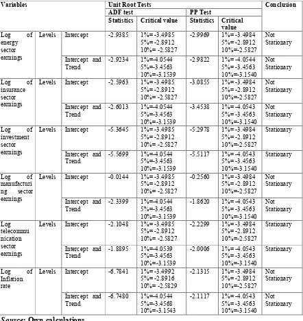
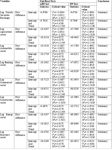
All variables were tested for non-stationarity. Augmented Dickey-Fuller (ADF) and
Philips-Peron (PP) test were used to test for the unit root with the data in logarithm form.
The results are in Table 4.2a and Table 4.2b.
Table 4.2a: Unit root results at levels
Variables Unit Root Tests Conclusion
ADF test PP Test
Statistics Critical value Statistics Critical
value
Log of Nairobi Securities Exchange index
Levels Intercept -1.35344 1%= -3.4977 5%= -2.8909 10%= -2.5825
-1.5360 1%= -3.4977 5%= -2.8909 10%=-2.5825
Not Stationary
Intercept and Trend
-1.53600 1%=-4.0534 5%=-3.4558 10%=-3.1537
-1.4511 1%= -4.0534 5%= -3.4558 10%=-3.1537
Not Stationary
Log of agriculture sector earnings
Levels Intercept -3.1094 1%= -3.4984 5%= -2.8912 10%= -2.5827
-3.2975 1%= -3.4984 5%= -2.8912 10%=-2.5827
Not Stationary
Intercept and Trend
-3.2507 1%=-4.0544 5%=-3.4563 10%=-3.1539
-3.4429 1%= -4.0543 5%= -3.4563 10%=-3.1540
Not Stationary
Log of automobile sector earnings
Levels Intercept -3.6057 1%= -3.4991 5%= -2.8916 10%= -2.5828
-3.4535 1%= -3.4984 5%= -2.8912 10%=-2.5827
Not Stationary
Intercept and Trend
-3.7094 1%=-4.0544 5%=-3.4563 10%=-3.1539
-3.5755 1%= -4.0543 5%= -3.4563 10%=-3.1540
Not Stationary
Log of banking sector earnings
Levels Intercept -1.8345 1%= -3.4985 5%= -2.8912 10%= -2.5827
-1.7205 1%= -3.4984 5%= -2.8912 10%=-2.5827
Not stationary
Intercept and Trend
-2.0992 1%=-4.0544 5%=-3.4563 10%=-3.1539
-2.1084 1%= -4.0543 5%= -3.4563 10%=-3.1540
Not Stationary
Log of commercial sector earnings
Levels Intercept -2.9004 1%= -3.4984 5%= -2.8912 10%= -2.5827
-2.9269 1%= -3.4984 5%= -2.8912 10%=-2.5827
Not Stationary
Intercept and Trend
-2.9224 1%=-4.0544 5%=-3.4563 10%=-3.1539
-2.9201 1%= -4.0543 5%= -3.4563 10%=-3.1540
Not Stationary
Log of constructio n sector earnings
Levels Intercept -2.7311 1%= -3.4985 5%= -2.8912 10%= -2.5827
-2.7538 1%= -3.4984 5%= -2.8912 10%=-2.5827
Not Stationary
Intercept and Trend
-1.9673 1%=-4.0544 5%=-3.4563 10%=-3.1539
-2.0692 1%= -4.0544 5%= -3.4563 10%=-3.1540